Bayesian Language Model based on Mixture of Segmental Contexts for Spontaneous Utterances with Unexpected Words

Bayesian Language Model based on Mixture of Segmental Contexts

for Spontaneous Utterances with Unexpected Words

Ryu Takeda Kazunori Komatani

The Institute of Scientific and Industrial Research, Osaka University 8-1, Mihogaoka, Ibaraki, Osaka 567-0047, Japan

{rtakeda, komatani}@sanken.osaka-u.ac.jp

Abstract

This paper describes a Bayesian language model for predicting spontaneous utterances. People sometimes say unexpected words, such as fillers or hesitations, that cause the miss-prediction of words in normal N-gram models. Our proposed model considers mixtures of possible segmental contexts, that is, a kind of context-word selection. It can reduce negative effects caused by un-expected words because it represents conditional occurrence probabilities of a word as weighted mixtures of possible segmental contexts. The tuning of mixture weights is the key issue in this ap-proach as the segment patterns becomes numerous, thus we resolve it by using Bayesian model. The generative process is achieved by combining the stick-breaking process and the process used in the variable order Pitman-Yor language model. Experimental evaluations revealed that our model outperformed contiguous N-gram models in terms of perplexity for noisy text including hesitations.

1 Introduction

1.1 Background

Language models (LMs) are widely used for text analysis, word segmentation and word prediction in automatic speech recognition (ASR). The basic LM is a conventional N-gram model that predicts a word depending on the patterns of the previousN words (context). The probability of a word is usually calculated by counting the words that match the context in text data as maximum likelihood estimation. Therefore, the model easily predicts frequent words or set expressions but not rare words or phrases.

VariousN-gram language models have been proposed to prevent the incorrect probability assignment caused by the increase of the context lengthN. Since the number of combinations ofN becomesO(VN) for vocabulary sizeV, there are a lot of patterns that do not appear in training data (data sparseness). Us-ing anN-gram model based on a Bayesian framework is a promising approach for data sparseness. Be-cause it is based on a Bayesian framework, an LM based on hierarchical Pitman-Yor process (HPYLM) has two main differences from previous language models (Teh, 2006), such as Witten-bell (WB) (Witten and Bell, 1991) and Kneser-ney (KN) smoothing (Kneser and Ney, 1995): 1) a Bayesian model express-ing conventional smoothexpress-ing methods and 2) automatic tunexpress-ing of parameters from data. Since HPYLM is based on a Bayesian framework, we can integrate other probabilistic models theoretically for other problems and apply optimization methods in accordance with a Bayesian framework. In contrast, other smoothing methods has several parameters that need to be tuned manually.

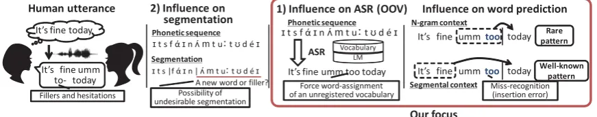
Human utterances contain various fillers and hesitations (left in Fig. 1), and these cause the mis-prediction of words because they rarely appear in the training data, that is, another type of sparsity. This will affect 1) the word prediction accuracy in ASR and 2) the precision of word segmentation (Mochi-hashi et al., 2009) or lexicon acquisition from speech signal (Elsner et al., 2013; Kamper et al., 2016; Taniguchi et al., 2016), which are our main interest. Since such hesitations are usually not registered

This work is licensed under a Creative Commons Attribution 4.0 International Licence. Licence details: http:// creativecommons.org/licenses/by/4.0/

/ƚ͛Ɛ ĨŝŶĞ ƵŵŵƚŽŽ ƚŽĚĂLJ

/ƚ͛Ɛ ĨŝŶĞ Ƶŵŵ ƚŽͲ ƚŽĚĂLJ /ƚ͛Ɛ ĨŝŶĞƚŽĚĂLJ

/ƚ͛Ɛ ĨŝŶĞ ƵŵŵƚŽŽ ƚŽĚĂLJ ZĂƌĞ ƉĂƚƚĞƌŶ

tĞůůͲŬŶŽǁŶ ƉĂƚƚĞƌŶ EͲŐƌĂŵĐŽŶƚĞdžƚ

^ĞŐŵĞŶƚĂůĐŽŶƚĞdžƚ DŝƐƐͲƌĞĐŽŐŶŝƚŝŽŶ ;ŝŶƐĞƌƚŝŽŶĞƌƌŽƌͿ /ƚ͛ƐĨŝŶĞƵŵŵƚŽŽƚŽĚĂLJ

ɪƚƐĨɳɪŶʌ́mƚƵƼƚʊĚĠɪ WŚŽŶĞƚŝĐƐĞƋƵĞŶĐĞ

>D ^Z sŽĐĂďƵůĂƌLJ

&ŽƌĐĞǁŽƌĚͲĂƐƐŝŐŶŵĞŶƚ ŽĨĂŶƵŶƌĞŐŝƐƚĞƌĞĚǀŽĐĂďƵůĂƌLJ

,ƵŵĂŶƵƚƚĞƌĂŶĐĞ ϭͿ/ŶĨůƵĞŶĐĞŽŶ^Z;KKsͿ /ŶĨůƵĞŶĐĞŽŶǁŽƌĚƉƌĞĚŝĐƚŝŽŶ

&ŝůůĞƌƐĂŶĚŚĞƐŝƚĂƚŝŽŶƐ

ϮͿ/ŶĨůƵĞŶĐĞŽŶ ƐĞŐŵĞŶƚĂƚŝŽŶ

ɪƚƐĨɳɪŶʌ́mƚƵƼƚʊĚĠɪ

WŚŽŶĞƚŝĐƐĞƋƵĞŶĐĞ

KƵƌĨŽĐƵƐ ɪƚƐͮĨɳɪŶͮʌ́mƚƵƼƚʊĚĠɪ

^ĞŐŵĞŶƚĂƚŝŽŶ

WŽƐƐŝďŝůŝƚLJŽĨ ƵŶĚĞƐŝƌĂďůĞƐĞŐŵĞŶƚĂƚŝŽŶ

ŶĞǁǁŽƌĚŽƌĨŝůůĞƌ͍

Figure 1: Problem caused by unexpected and inserted words

to an ASR vocabulary (out-of-vocabulary; OOV), they are recognized as the most similar and likely word in the vocabulary set in terms of pronunciation and context (middle-right in Fig. 1). Moreover, mis-recognized words may also affect the subsequent word prediction based onN-gram auto-regression. Such mis-recognition is a kind of insertion error caused by fillers, hesitations and other noise signals, such as coughs. For example, the hesitation “to-” is recognized as “too”, and the filler “umm” and hes-itation “too” are used for the prediction of the next word if we use normalN-gram model (right upper in Fig. 1). Note that hesitations are hard to eliminate by using only a filler-word list because their com-plete patterns cannot be prepared in advance. As for word segmentation and lexicon acquisition, the language model is trained from character/phoneme sequences or raw speech signal in anunsupervised

manner. The Bayesian nonparametrics is often applied to this problem because it enables us to control the number of words/symbols dynamically according to the amount of data. Since the lexicon acquisi-tion includes a kind of segmentaacquisi-tion problem, fillers and hesitaacquisi-tions may cause mis-segmentaacquisi-tions. A nonparametric generative model that can deal with hesitations and fillers will help to recognize words sequence and segment words from phoneme sequence.

We propose using a Bayesian language model in which probability consists of a mixture of condi-tioned probabilities of segmental contexts for the word prediction problem. Since the lexicon acquisition from phonetic sequence or rawconversationalspeech signal is also our scope, Bayesian approach is nec-essary in terms of scalability. Our model removes (ignores) some words, such as fillers and hesitations in the ideal case, from the context in predicting words. For example, given the text “It’s fine umm too to-day,” the probabilityp(today|It’s,fine,umm,too)is defined as a mixture ofpˆ(today|It’s,fine,umm,too),

ˆ

p(today|fine,umm),pˆ(today|It’s,fine)and so on (right lower Fig. 1). The risk of mis-prediction caused by the unknown context is reduced by other differently conditioned probabilities. Since the given term includes many patterns of segmental context, we constrain the pattern to one “contiguous” segment. That is, the probabilities of a discontiguous segment, such asp(today|It’s,umm), are not included in the mixture. Since the generative process can be expressed by combining the stick-breaking process (Sethu-raman, 1994) and the process used in the variable order Pitman-Yor language model (VPYLM) (Mochi-hashi and Sumita, 2007), the parameters can be estimated by Gibbs sampling (Christopher Michael Bishop, 2006) the same as they are for VPYLM.

1.2 Related Work on Mixture Models

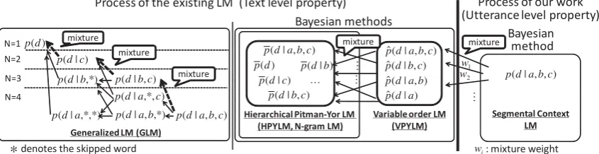
The main differences between our work and previous studies are 1) assumed context patterns in the mixture and their purpose (text-level or utterance-level), and 2) whether the model is Bayesian or not. Our proposed model is one of various mixture language models and there are several language mixture models that consider word dependency. Again, we stochastically ignoresome contiguous words in the context in accordance with the appearance of fillers, hesitations and noises (right in Fig. 1) at the utterance-level. Since other LM models correspond to the process for text generation in our framework, we can embed them in our process as mixture components if necessary. As shown in the right half of Fig. 2, our current model is based on the mixture of VPYLM which is based on the mixture of HPYLM. Note that VPYLM and HPYLM have no mechanism to select words in the context for prediction.

lan-) , , | (d abc p ) , | (d bc p

) ,*, | (d a c p

,*) , | (d ab p ) | (d c p

,*,*) | (d a p

,*) | (d b p ) (d p ) , , | (d abc p )

, | ( ˆd bc p

) , | ( ˆd ab p

) | ( ˆd a p )

| (d c p

) (d

p p(d|b)

) , , | ( ˆ d abc p

) , | (d bc p

sĂƌŝĂďůĞŽƌĚĞƌ>D ;sWz>DͿ ,ŝĞƌĂƌĐŚŝĐĂůWŝƚŵĂŶͲzŽƌ >D

;,Wz>D͕EͲŐƌĂŵ>DͿ ^ĞŐŵĞŶƚĂůŽŶƚĞdžƚ>D )

, , | (d abc

p ŵŝdžƚƵƌĞ Eсϰ Eсϯ EсϮ ŵŝdžƚƵƌĞ ŵŝdžƚƵƌĞ ŵŝdžƚƵƌĞ WƌŽĐĞƐƐŽĨƚŚĞĞdžŝƐƚŝŶŐ>D;dĞdžƚůĞǀĞůƉƌŽƉĞƌƚLJͿ WƌŽĐĞƐƐŽĨŽƵƌǁŽƌŬ ;hƚƚĞƌĂŶĐĞůĞǀĞůƉƌŽƉĞƌƚLJͿ L Eсϭ ŵŝdžƚƵƌĞ 'ĞŶĞƌĂůŝnjĞĚ>D;'>DͿ M M *ĚĞŶŽƚĞƐƚŚĞƐŬŝƉƉĞĚǁŽƌĚ 1 w 2 w M i w͗ŵŝdžƚƵƌĞǁĞŝŐŚƚ ĂLJĞƐŝĂŶŵĞƚŚŽĚƐ ĂLJĞƐŝĂŶ ŵĞƚŚŽĚ ĚĞŶŽƚĞƐƚŚĞĐŽŶƚĞdžƚƉĂƚƚĞƌŶƵƐĞĚŝŶtĂŶĚ<E

Figure 2: Language model structures: GLM (left), HPYLM/VPYLM (middle) and our model (right)

guage model (GLM) that mixes all probabilities of possible context patterns ofN-grams hierarchically (Pickhardt et al., 2014). At each context depth, a word isskippedin the context (skipN-gram (Goodman, 2001; Guthrie et al., 2006)), and the probability is smoothed by shallow contexts. The relative position in the context remains, and the skipped word is denoted by the asterisk ∗. WB and KN use only the contiguous contexts for smoothing as shown in the Figure. Wu and Matsumoto (2015) proposed a hier-archical word sequence language model using directional information. The most frequently used word in the sentence is selected for splitting a sentence into two substrings, and a binary-tree is constructed by a recursive split. If a directional structure is assumed, the context patterns decrease in size and the processing time is shortened.

Running a language model on a recurrent neural network (RNN) (Mikolov et al., 2010) is, of course, a reasonable choice because of the good prediction performance for closed-vocabulary task. However, a neural network LM usually does not include a generative process, so it is difficult to apply to unsu-pervisedtraining of a language model or lexicon acquisition from speech signals. In that sense, the LM based on generative model is still important. Of course, the combination method of Bayesian model and neural networks should be investigated for practical use.

Our work is the extension of VPYLM based on mixture of segmental contexts to deal with hesitations and fillers. And our mixture pattern is designed for hesitation and fillers, and it is simpler than that of others in terms of the number of context patterns.

2 Hierarchical Bayesian Language Model based on Pitman-Yor Process

This section explains the fundamental mechanism of a language model based on Bayesian nonparamet-rics. HPYLM should predict words more accurately than KN-smoothing because KN-smoothing is an approximation of this model.

2.1 Generative Model

The N-gram LM approximates the distribution over sentences w_T, ..., w₁ using the conditional distri-bution of each word w_t given a context h consisting of only the previous N − 1 words wt_N−₋1₁ =

{wt−1, ..., wt−N+1},

p(wT, ..., w1) =

T

t

p(wt|wtN−−11). (1)

The trigram model (N = 3) is typically used. Since the number of parameters increases exponentially asN becomes larger, the maximum-likelihood estimation severely overfits the training data. Therefore, smoothing methods are required if vocabularyV is large.

If he/she selects a new table, an agent of the customer recursively enters the parent restauranthas a new customer. Here, we represent the depth ofhas|h|, and there is the relationship|h|=|h|−1. Given the seating arrangement of customerss, the conditional probability of wordwwith the contexthis defined as follows

p(wt|s,h) = ch_cw−d|h|thw

h∗+θ|h| +

θh+d|h|th∗

ch∗+θ|h| p(wt|s,h

_{), (2)}

wherec_hwis the count of wordwat contexth, andc_h∗=_wc_hwis its sum. t_hwis the number of table at contexth, andt_h∗is also its sum. θ_|h|andd_|h|are the common parameters ofhwith the same depth

|h|. The distribution over the current word given the empty contextφis assumed to be uniform over the vocabulary wofV words. The variable order PYLM integrates out the context length (depth)N, thus we need not determine the length in advance.

The predictive probability of wordwis approximated by averaging Eq. (2) over sampled seating ar-rangements_n(n= 1, ..., N).

p(w|h) = 1 N

n

p(w|sn,h) (3)

2.2 Inference of Parameters

The latent variablesand other parametersdandθare obtained through simulations on the basis of Gibbs sampling given training textw¯_i(i= 1, ..., N_train). The procedure for sampling a customer is as follows:

1. Add all customers to the restaurants

2. Select a certain customerw¯_i

3. Remove the customer from the restaurant. If a table becomes null, also remove the agent from the parent restaurant recursively.

4. Add the customer to the leaf restaurant. He chooses a table with probabilities proportional to the number of customers at each table. If the table is null, also add an agent to the parent restaurant recursively. (Go back to Step 2).

The parameters are sampled using auxiliary variables from their posterior probability. Please see the work of Teh (Teh, 2006) for the detailed sampling algorithm.

2.3 Problem of Contiguous Context Model

TheN-gram model is modeled as a series of words, and has an advantage in expressing common phrases. The Bayesian nonparametrics enables the N-gram model to tune the smoothing parameters automati-cally. This improves the accuracy of predicting rare words in a large context.

Unexpected words degrade the prediction accuracy of theN-gram model. The unexpected words in-clude noises, fillers, and hesitations in actual utterances. For example, the probability ofp(sing|he,will) is estimated reliably. However, the probability ofp(sing|will,sh..), which includes a hesitation (“sh..”), is estimated unreliably because the hesitation does not appear in the corpus. The patterns of insertion location and bursty are also not determined in advance.

3 Bayesian Language Model based on Mixture of Segmental Contexts

? =

t

w 1

−

t

w 2

−

t

w 3

−

t

w 4

−

t

w

ƐƚŽƉ 5

−

t

w

ƐƚŽƉ

^ĂŵĞƉƌŽĐĞƐƐŽĨsWz 6

−

t

w

ĐŽŶƚĞdžƚ

/ŐŶŽƌŝŶŐƉƌŽĐĞƐƐ

L

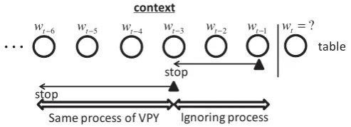
Figure 3: Process for segmental context model

3.1 Generative Model

We assume that the conditional distribution of each wordw_tgiven a context is a mixture of the segmental

N-gram context. The segmental N-gram is a part of context w_t−i, .., w_t−j, which begins at w_t−i and ends atw_t−j.

p(w|wt_N−₋1₁) =

i

j>i

p(w|w_Nt−₋1₁, i, j)p(i, j) =

i

j>i

p(w|wt_j−i)p(j|i)p(i) (4)

If we consider theN → ∞, the possible segmental patterns are also considered. Setting the start index

iofN-gram appropriately can eliminate the influence of the sequential unexpected words for predicting the next word. The word probability termp(w_t|wt_j−i)is determined by HPYLM.

The stick-breaking process (SBP) represents the generative process of Eq. (4) as the same way of VPYLM (Mochihashi and Sumita, 2007). The process consists of two parts; 1) decide the start indexi ofN-gram and then 2) decide the end indexj ofN-gram. Each index is determined probabilistically using SBP (Fig. 3).

Step1 - Process for start indexi: First, the customer walks along the tables (word) from the start,w_t−1. The customer stops at thei-th table with probabilityη_i, and passes it with probability1−η_i. Therefore, the probability that the customer stops at thei-th table is given by

p(i|η) =ηi i−1

l=1

(1−ηl). (5)

This probability decreases exponentially. We assume that the prior of parametersηis Beta distribution Beta(α₁, β₁).

Step2 - Process for end index j: The end index j is also determined using the same process i. The customer walks along the tables from thei-th table, and stops at or passes thej-th table with probability

ζj or1−ζ_j, respectively.

p(j|i,ζ) =ζj j−1

l=1

(1−ζl). (6)

The prior of parametersζ is also assumed to be the Beta distribution Beta(α₂, β₂).

In fact, the whole process can be considered to be the combination of VPYLM and the start index determination process. We thus can describe the probability as

p(wt|wt∞−1) =

i

Pvpy(w|w_∞t−i−1)p(i). (7)

Table 1: Parameters of experiment

Artificial noisy data Actual hesitation data

English Japanese Japanese

Target text War and Peace CSJ CSJ

Training 27876 sentences 110566 sentences 114372 sentences 479585 words 2828499 words 3084592 words Test for clean 5128 sentences 7134 sentences 20440 sentences 88552 words 199100 words 184145 words Test for noisy 5128 sentences 7134 sentences 2296 sentences

97373 words 218945 words 32342 words

Vocabulary size 10717 18357 19703

(α1,β1) (9, 1) (1, 1)

(α2,β2) (1, 9) (1, 8)

3.2 Inference of Start Index

We assume that all words in training dataw¯ have the start indexi_tas a latent variable, and are estimated stochastically by Gibbs sampling. The start index i_tof the wordw¯_t is sampled given dataw¯, seating arrangements, and start and end indexes of other wordsi_−tandj_−tas

it ∼ p(it|w¯,s−t,j−t,i−t) (8)

∝ p(wt|w¯−t,j−t,i)p(it|w¯−t,s−t,i−t,j−t) (9)

where the notation−tmeans that thet-th element corresponding tow¯_tis excluded. Here, the first term,

p( ¯wt|w¯−t,j−t,i), is calculated using VPYLM because the start indexitis given. The second term is a prior probability to select the start index. It can be calculated in the same way used in the VPYLM:

p(it=l|w−t,s−t,i−t,j−t) = _a al+α1 l+bl+α1+β1

l

k=1

bk+β1

ak+bk+α1+β1, (10)

whereα₁andβ₁are hyper-parameters of the Beta distribution. Thea_landb_lare the count of customers who stopped at and those who passed tablew¯_l. This probability is assumed to depend only onw¯_l, not whole contexth. Since the probability of the word corresponding tow¯_lis not important for the prediction is low, the effect of an unexpected word on this index is reduced.

Once the start index is set, we can also draw the end indexj_tand the seating arrangements_tthrough VPYLM process. Thej_tis first drawn from its posterior distribution, and then seatings_tis also drawn from its posterior distribution. After sampling, the average word probability is used for prediction.

The computational cost of our model is proportional toO(N)while the cost of the generalized lan-guage model is roughly proportional to O(2N). The enumeration of all combinations of words that should be used is computationally heavy for models based on Bayesian nonparametrics when N be-comes larger and we optimize parameters of the model. Moreover, the context pattern of the generalized model is complex to deal with fillers and hesitations (insertion errors).

4 Experimental Evaluations

4.1 Experimental Setup

We used two kinds of text for evaluation: 1) artificial noisy text and 2) actual hesitation text (Japanese only). The former is for the validation of our method with model-matched data, and the latter is for the performance measurement with real utterances.

We used two languages English and Japanese text data for training and test dataset for the artificial noisy text. The English text was “War and Peace” from project Gutenberg1, and the Japanese text was the Corpus of Spontaneous Japanese (CSJ2), consists of transcriptions of Japanese speech. For the English

1

http://www.gutenberg.org/ 2

text, we randomly selected 27,876 sentences from the entire of “War and Peace” for training data, and used the remaining 5,128 sentences for test data. For Japanese text, we used 110,566 sentences in the “non-core” set for training data and 7,134 sentences in the “core” set for test data. All hesitations and fillers were eliminated from the Japanese corpus to make it formal text data3. The utterances in the CSJ that have0.5-second short-pauses were separated into sub-utterances, and each sub-utterance was treated as a sentence. The words that appeared more than once were selected for the vocabularies. The sizes of vocabularies were 10,717 words for English text and 18,357 words for Japanese text. To simulate the artificial noisy text, we added words randomly selected from vocabularies into the test data at a rate of 10 %. The OOVs in the test set were treated as a symbol, “<unk>”.

The raw CSJ Japanese transcription text was used for the actual hesitation text. In this experiment, hesitations and fillers in the training set arenoteliminated. The utterances that have0.2-second short-pauses were separated into sub-utterance, and each sub-utterance was treated as a sentence. The 0.2 -second is selected to make a rate of hesitation in noisy text about8.0%. The test transcription data (“core” set) were divided into two categories: hesitation-included noisy text (2,296 sentences) and clean text (20,440 sentences). The number of hesitations in the test dataset was 2649 (about2649/32342 = 8.1% ). The hesitation-included noisy text included hesitations, so its vocabulary was 19,703. The out of vocabulary (OOV) words in the hesitation test data were replaced by words randomly selected from the vocabulary set that had a phoneme distance to the OOV word of less than 2. This is because such OOV words including unknown hesitations are actually mis-recognized and assigned similar-sounding words in the ASR vocabulary. Therefore, the vocabulary set was closed. Note thatfrequent fillers and hesitations remained in both the test and training sets. These settings are listed in Tab. 1.

We compared our model with other models: WB, KN, Modified KN (MKN) (Chen and Goodman, 1999), HPYLM, and VPYLM. The hyper-parameters,α₂andβ₂of the Beta distribution used in VPYLM were set to1and9for the artificial data, and1and8for the actual hesitation data. Additionally, those of the start index process,α₁andβ₁, were set to9and1for the artificial data, and1and1for the actual hesitation data. These parameters were selected to perform best for each test set to evaluate the limitation of methods. For the English and Japanese text,N was set to3,4,6,10. For the Japanese transcription, it was set to 3, 6, 8, 10. The predictive probability was averaged over 30 seating arrangements after 90 iterations of Gibbs sampling. We also investigate the performance of RNN language model 4 as a reference. We tried several parameter set of RNN, such as the number of hidden layers and classes, and they are also tuned for each test set. Note that the main interest of our experiments is the performance comparison among Bayesian methods.

Perplexity (PP) was used as the evaluation criterion.

PP= 2P(wtest), P(w_test) =− 1

Ntest

s∈w_test

logP(s), (11)

wheresis a sentence in the test data andN_{test is the number of words in the test dataset. The PP was} calculated under the assumption that each sentence was independent. Smaller PP values mean better word prediction accuracy. The prediction of OOVs, which are denoted by “<unk>”, in the artificial test set is eliminated in calculating perplexity.

4.2 Results and Discussion

4.2.1 Artificial Noisy Data

The perplexity values for the two data sets and the fourN-gram lengths can be seen in Tabs. 2 and 3 for English and Japanese text, respectively. The clean text denotes the raw formatted text, and the noisy text denotes the ones with randomly-added words. There is no noteworthy difference between the English and Japanese text other than the range of PP.

The differences among methods for clean text data withN = 3are clear. Like in the results of previous studies, HPYLM and MKN had the lowest PP, followed by VPYLM and WB. Our model had worse PP

3

All words were tagged by hand. The tags of fillers and hesitations were included. 4

Table 2: Perplexity for English text

maximum context lengthN

Test dataset Method 3 4 6 10

Clean text

WB 167.9 163.8 163.2 163.2 KN 152.7 150.9 157.9 157.8 MKN 153.1 151.3 156.7 157.9 HPYLM 155.0 151.6 151.5 151.6 VPYLM 156.0 153.3 153.2 153.2 Ours 161.7 154.6 152.7 152.9

RNN 135.4

Noisy text

WB 365.9 360.0 359.2 359.2 KN 328.3 322.4 331.2 332.5 MKN 321.4 316.5 328.2 331.8 HPYLM 326.0 321.8 321.5 321.6 VPYLM 327.4 324.0 324.1 324.2 Ours 322.4 309.5 306.0 306.0

RNN 312.0

Table 3: Perplexity for Japanese text

maximum context lengthN

Test dataset Method 3 4 6 10

Clean text

WB 56.6 55.8 56.6 56.9

KN 53.1 50.7 50.4 51.4

MKN 52.3 50.0 49.4 50.3 HPYLM 52.1 50.0 49.5 49.5 VPYLM 52.2 50.5 50.0 49.9 Ours 53.1 51.0 50.4 50.5

RNN 46.1

Noisy text

WB 180.7 178.9 180.4 181.0 KN 174.0 166.1 163.4 165.0 MKN 164.4 158.3 156.3 159.3 HPYLM 160.9 156.9 156.1 156.0 VPYLM 158.8 155.0 153.3 152.4 Ours 147.0 143.2 143.2 144.3

RNN 166.1

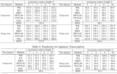
Table 4: Perplexity for Japanese Transcription

maximum context lengthN

Test dataset Method 3 6 8 10

Clean text

WB 61.3 62.1 62.3 62.4 KN 57.6 55.5 56.1 56.4 MKN 53.9 56.8 54.8 54.0 HPYLM 56.3 54.5 54.5 54.5 VPYLM 56.4 54.7 54.7 54.7 Ours 57.4 55.0 55.0 55.0

RNN 46.0

maximum context lengthN

Test dataset Method 3 6 8 10

Noisy text

WB 102.4 104.4 104.8 104.9

(hesitations)

KN 95.6 92.2 93.2 93.7

MKN 93.1 89.5 89.8 90.6 HPYLM 91.3 89.0 89.1 89.0 VPYLM 91.2 89.0 89.0 89.1 Ours 91.8 88.2 88.1 88.2

RNN 83.1

than MKN, HPYLM and VPYLM. Since our model stochastically ignores some contiguous words in the context, the prediction accuracy for formatted text was worse than those of other methods. This can be reduced by using more text data or an improved model discussed in the next subsection. Using a longer context improved the PPs of HPYLM and our model. Therefore, a longer context is useful for word prediction. The perplexity of RNN was smallest, and RNN outperformed others by 15 and 4 points for English and Japanese text.

The ranking were different for the noisy text data. The relative performances of WB, KN, MKN, HPYLM, and VPYLM were almost the same as those for the clean text, but our model had the lowest PP. Its performance improved with the context length N = 6 or10. The perplexity of RNN is also higher than that of our model. This indicates that the segmental context mixture works as intended, i.e. reducing the negative effect of unknown context. The improvement with a longer context means that Bayesian smoothing works well.

4.2.2 Actual Hesitation Data

The perplexity values for the fourN-gram lengths can be seen in Tab. 4 for clean sentences and hesitation included sentences. The perplexity was much higher for all four models with the noisy text mainly due to hesitations and substitution errors caused by OOVs. Therefore, the word-prediction for actual utterance is more difficult than written text.

ŽŶ͛ƚ ǁŽƌŬ ŵƵŵ ƚŽŽ ŚĂƌĚ

ŽŶ͛ƚ ǁŽƌŬ ŵƵŵ ƚŽŽ ŚĂƌĚ

ŵŝƐͲƌĞĐŽŐŶŝƚŝŽŶ

^ƚĞƉƚ͗

;'ŽŽĚƐŝƚƵĂƚŝŽŶͿ ^ƚĞƉƚнϭ͗

;ĂĚƐŝƚƵĂƚŝŽŶͿ ͞ƚŽŽ͟ƐŚŽƵůĚďĞƵƐĞĚ ĨŽƌƉƌĞĚŝĐƚŝŽŶ

ĐŽŶƚĞdžƚ

ƚĂŝů

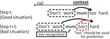
Figure 4: Weakness of segmental context model

suffered from the contiguous noisy words that were caused by the combination of the noise word and OOVs, “<unk>”, in the artificial noisy data, and RNN degraded prediction accuracy for artificial noisy data. This indicated that RNN is unfamiliar to open-vocabulary tasks, such as lexicon acquisition.

The model validation with these text-level experiments provides us important knowledge and signif-icant results for the next-level research step. Our method will be more effective for the word/phoneme segmentation problem because the substitution of hesitations to OOVs does not happen and we have to handle raw hesitation symbols. For example, the hesitation “to-” will be treated as itself “to-” or a pho-netic expression “t u:”, and the skip prior/posterior probability Eq. (6) and (9) of a hesitation symbol will be estimated properly. Our model will provide criteria for which words or symbols should be skipped. Therefore, the model integration of ours and the OOV-free model (Mochihashi et al., 2009) is required to process actual conversational utterances.

4.2.3 Remaining Problem on Model

The main problem of our model is clear from these results: it completely ignores neighbor context and does not use it for prediction, as illustrated in Figure 4. Since the neighbor words are usually useful for prediction, ignoring such words will degrade perplexity, especially that of clean text. The actual fillers/hesitations and mis-recognized words move from head to tail in the context in predicting words sequentially. Therefore, if the unknown segment is away from the context root, we can use the neighbor context without risk. For example, the probabilitypˆ(hard|work,mum,too)should be a mixture ofp(hard|work,mum),p(hard|work,too),p(hard|too) and so on. The probabilityp(hard|work,too)is not considered in our current model. By modeling this property, our model will perform the same as HPYLM and VPYLM for clean text.

The future work also includes the fundamental modification of our model and the application to word/phoneme segmentation problem of actual utterances. Since hesitation is often a part of phoneme sequence of a word, it also depends on the currently or previously uttered word. A new generative process modeling above properties is required to deal with conversational utterances.

5 Conclusion

We proposed a segmental context mixture model to reduce the prediction error caused by noises, fillers, and hesitations in utterances, which rarely appear in the training text. Although hesitations or fillers will appear for speech transcriptions, they vary according to a speaker and topic. The model’s probability consists of a mixture of conditioned probabilities of part of context words. The generative process can be expressed by combining the stick-breaking process and the process used in the variable order Pitman-Yor Language model (VPYLM). Experimental results revealed our model had better perplexity for noisy text than hierarchical PYLM, VPYLM, Witten-Bell and Kneser-ney smoothing.

Acknowledgements

This work was supported by JSPS KAKENHI Grant Number 15K16051.

References

Stanley F Chen and Joshua Goodman. 1999. An empirical study of smoothing techniques for language modeling.

Computer Speech & Language, 13(4):359–394.

Christopher Michael Bishop. 2006. Pattern Recognition and Machine Learning. Springer-Verlag New York.

Micha Elsner, Sharon Goldwater, Naomi Feldman, and Frank Wood. 2013. A joint learning model of word segmentation, lexical acquisition, and phonetic variability. InIn proc. of the Conference on Empirical Methods on Natural Language Processing, pages 42–54.

Joshua T. Goodman. 2001. A bit of progress in language modeling. Computer Speech & Language, 15(4):403–

434.

David Guthrie, Ben Allison, Wei Liu, Louise Guthrie, and Yorick Wilks. 2006. A closer look at skip-gram

modelling. InProc. of the 5th international Conference on Language Resources and Evaluation, pages 1222–

1225.

Herman Kamper, Aren Jansen, and Sharon Goldwater. 2016. Unsupervised word segmentation and lexicon

dis-covery using acoustic word embeddings. IEEE/ACM Trans. on Audio, Speech, and Language Processing,

24(4):669–679.

Reinhard Kneser and Hermann Ney. 1995. Improved backing-off for m-gram language modeling. InProc. of

International Conference on Acoustics, Speech, and Signal Processing, volume 1, pages 181–184.

Tomas Mikolov, Martin Karafi´at, Lukas Burget, Jan Cernock`y, and Sanjeev Khudanpur. 2010. Recurrent neural

network based language model. InProc. of Interspeech, pages 1045–1048.

Daichi Mochihashi and Eiichiro Sumita. 2007. The infinite markov model. InAdvances in Neural Information

Processing Systems, pages 1017–1024.

Daichi Mochihashi, Takeshi Yamada, and Naonori Ueda. 2009. Bayesian unsupervised word segmentation with

nested pitman-yor language modeling. InProc. of the Joint Conference of the 47th Annual Meeting of the ACL

and the 4th International Joint Conference on Natural Language Processing of the AFNLP: Volume 1-Volume 1, pages 100–108.

Rene Pickhardt, Thomas Gottron, Martin K¨orner, Steffen Staab, Paul Georg Wagner, and Till Speicher. 2014. A generalized language model as the combination of skipped n-grams and modified kneser ney smoothing. In

Proc. of the 52nd Annual Meeting of the Association for Computational Linguistics, pages 1145–1154.

Jayaram Sethuraman. 1994. A constructive definition of dirichlet priors. Statistica Sinica, pages 639–650.

Tadahiro Taniguchi, Shogo Nagasaka, and Ryo Nakashima. 2016. Nonparametric bayesian double articulation

analyzer for direct language acquisition from continuous speech signals. IEEE Transactions on Cognitive and

Developmental Systems, 8(3):171–185.

Yee Whey Teh. 2006. A bayesian interpretation of interpolated kneser-ney. Technical Report TRA2/06, School of

Computing, NUS.

Ian H Witten and Timothy C Bell. 1991. The zero-frequency problem: Estimating the probabilities of novel events

in adaptive text compression.IEEE Trans. on Information Theory, 37(4):1085–1094.

Xiaoyi Wu and Yuji Matsumoto. 2015. An improved hierarchical word sequence language model using directional

information. InProc. of The 29th Pacific Asia Conference on Language, Information and Computation, pages