Data-driven learning of symbolic constraints for a log-linear model in a
phonological setting
Gabriel Doyle Department of Psychology
Stanford University Stanford, CA 94305
Roger Levy
Department of Brain and Cognitive Sciences Massachusetts Institute of Techonology
Cambridge, MA 02139
Abstract
We propose a non-parametric Bayesian model for learning and weighting symbolically-defined constraints to populate a log-linear model. The model jointly infers a vector of binary con-straint values for each candidate output and likely definitions for these concon-straints, combining observations of the output classes with a (potentially infinite) grammar over potential constraint definitions. We present results on a small morphophonological system, English regular plurals, as a test case. The inferred constraints, based on a grammar of articulatory features, perform as well as theoretically-defined constraints on both observed and novel forms of English regular plurals. The learned constraint values and definitions also closely resemble standard constraints defined within phonological theory.
1 Introduction
Constraint-based models of language, often in the form of “maximum entropy” or “log-linear” models, are prominent in many applications and theoretical analyses in computational linguistics and psycholin-guistics, including in text segmentation (Beeferman et al., 1999; Poon et al., 2009), machine translation (Och and Ney, 2002), syntactic alternation choice (Bresnan et al., 2007), and phonology (Goldwater and Johnson, 2003). Building successful models – and learning about human behavior from them – relies on the ability to identify relevant constraints, and this can be a difficult problem.
In this paper, we propose a system for learning both the values of and symbolic definitions for such constraints. We present a framework that combines observed data about linguistic outcomes with a flexible probabilistic context-free grammar of constraint structure to jointly infer (binary) feature values for multiple constraints and likely symbolic definitions for those constraints. We ground the model in a morphophonological setting, using the model to infer what phonological constraints affect the output form of regular English plurals, although it can be applied to other problems for which a constraint grammar can be defined.
The inference procedure moves beyond existing methods for learningextensionaldefinitions of con-straint values (Griffiths and Ghahramani, 2005; G¨or¨ur et al., 2006; Doyle et al., 2014) from observational data to incorporate top-down information about likelyintensionalconstraint definitions, improving both the applicability of the constraints and the theoretical basis for their values. We show that learning the constraints through this model performs as well as using pre-specified phonologically-standard con-straints in explaining both observed and novel regular plural morphophonology. In addition, the structure of the learned constraints is similar to standard phonological constraints, showing that the model can be useful in both applications and theory-building.
2 Constraint-based models and the phonological test case
Our core problem is how to learn appropriate identities and weights for log-linear features in linguistic applications. In general, we assume some set of input types{xi}, withni· instances of each type
ob-served. The input typexi is observed to producenij instances of each outcome typeyj, and, as we are
using a log-linear model, we assume that the number of observed input-output pairs(xi, yj)is
propor-tional to the exponential of the weighted sum of the constraint valuesvijkover all constraintsk. At least
some subset of these constraintskare unknown, and our goal is to learn the number of and values for these unknown constraints, as well as weights for both the known and unknown features.
Furthermore, we assume that the values of the unknown constraints are based on definitions that are generated from a symbolic grammar. This allows the model to inject theory- or observation-based struc-ture into the learning process, improving the plausibility of the constraint values and allowing the re-searcher to identify likely definitions for the constraints to apply to unobserved inputs. At present, we limit ourselves to the case where the unknown constraints are binary and depend only on the outcome typeyj, a simplified case that is particularly relevant to phonological constraint acquisition. We discuss
avenues for relaxing the binarity limitation in Section 7.
Gaps in log-linear phonological modeling We consider phonological theory as a test case because it has a well-established constraint-based framework, Optimality Theory (OT; Prince and Smolensky (1993)). But there is a gap in learning methods for OT-style phonology. Multiple methods have been proposed within OT for learning constraint weights or orderings (Tesar and Smolensky, 2000; Boersma and Hayes, 2001; Goldwater and Johnson, 2003) when the constraint definitions are known. None of these can learn constraint definitions, though three general tracks of research have pushed toward this goal. One track builds phonetically-grounded constraints based on the difficulty of producing or under-standing the sound sequences (Hayes, 1999), but cannot produce constraints that lack such grounded motivations (Hayes, 1995). A second track learns constraints within a phonotactic problem, looking solely at attested output forms (Hayes and Wilson, 2008; Berent et al., 2012), but the phonotactic learn-ing problem does not take input forms into account, and searches over a finite constraint set (instead of an infinite grammar). A third track uses data-driven learning to infer constraints (Doyle et al., 2014), but this method only learns which words violate a given constraint, and not a symbolic or intensional definition to apply it to novel words.
We propose a model to fill the gaps between these research tracks, by inferring constraints: 1) in the absence of articulatory motivation, 2) in the presence of input forms, and 3) with explicit, symbolic con-straint definitions. The model uses a simple (but infinite) grammar of concon-straints to jointly learn a matrix of constraint violations, likely definitions for the constraints, and relative weights on the constraints that adequately explain the observed phonological forms.
Phonological constraints and log-linearity Traditional versions of OT do not employ log-linearity, so we work with the MaxEnt OT (MEOT; Goldwater and Johnson (2003)) framework, an extension that connects constraint-based phonology to the general class of log-linear models. (Traditional, non-log-linear, OT is approximated as the difference between weights on the MEOT constraints grow.) Some existing work on phonotactic and phonological constraint learning (Hayes and Wilson, 2008; Doyle et al., 2014) has been based in such a log-linear framework.
As with all OT frameworks, the core structure supposes that phonological forms are produced by starting with an input form, generating a set of output candidates, determining what constraints each candidate input-output pair violates, and selecting an output form based on the number and strength of the candidates’ constraint violations. There are two types of constraints: those that depend on both the input and output (“faithfulness”), and those that depend only on the output (“markedness”). Each constraint has an associated weight, which is always non-positive; no constraint violations can make an output form more likely to be chosen. MEOT is a log-linear model, so summing the weights of all violated constraints provides each candidate’s linear predictor, which is logit-transformed to a probability.
In terms of the general framework from the start of this section, faithfulness constraints are known, while the markedness constraints and weights for both constraint types are unknown.1 In addition, we assume that the definitions for the markedness constraints are generated by a PCFG over phonological features of the sounds of the output candidates. Our specific grammar is discussed in Sect. 5.2.
1We limit ourselves to the learning of markedness constraints in this paper, as faithfulness constraints appear to be less
3 Model structure
We represent the constraints as two matrices: F, the observed faithfulness constraints, which depend on both input and output forms; andM, the unobserved markedness constraints, which depend only on the output form. Each cell ofF andM tells the number of violations of a constraint by a given input-output mapping. Fijkis the number of violations of faithfulness constraintkby input-output pair type(xi, yj);
Mjl is the number of violations of markedness constraintlby output candidateyj. For each inputxi,
some subset of the output forms{yj}are possible; this subset will be denotedY(xi). The weight vector
wprovides weights for bothF andM, and is unobserved.
M is a non-parametric binary matrix with a known number of rows (candidates) but an unknown num-ber of columns (constraints). Each columnM·lof the matrixM, which we will refer to as a “violation
profile”, is a binary vector of lengthJ, the number of output candidates, specifying whether the candi-dateyjviolates this constraint.wis a vector of real numbers; within OT, weights are strictly negative, so
we draw from−exp(ηw).
Previous work on constraint learning (Doyle et al., 2014) generatedM through an Indian Buffet Pro-cess (Griffiths and Ghahramani, 2005), with the number of constraintsLgenerated by a Poisson prior (with parameterα) and the violation profiles generated by a rich-get-richer scheme. In the present work, we retain the Poisson prior overL, but we want the violation profiles to be derived from symbolic con-straint definitionsdinstead. The definitions are built from the underlying grammarGand specify whether each candidateyj violatesd. Within our model, we assume that a candidateyj can be an exception to
the definitiond(switching a one to zero or vice versa inMjl), and the number of exceptions is drawn
from a exponential prior (Rational Rules framework; Goodman et al. (2008)). Thus, given a constraint definitiondl, the probability of it producing a violation profileM·lis given by
p(M·l|d)∝exp(−bQ(M·l;y·, dl)) (1)
whereQ(M·l;y·, dl)is the number of exceptions inM·lgiven candidates{yj}and definitiondl, andbis
the exception parameter, with largerbpenalizing exceptions more strongly. As neither the true violation matrixM nor the true constraint definitionsdare observed, we estimate the probability of a violation profileM·lby marginalizing over possible constraint definitions (see Sect. 4.1).
The probability of whole observed corpus Y is the product of the probabilities across all observed input-output pairs:
dl ∼ PCFG(G). We infer likely constraint matrices and weightsM andw from their joint posterior
distribution, which is proportional to the product of the probabilities of the data (Eqn. 2), constraintsM, and weightsw:
p(M, w|Y, F, α, b, ηw, G)∝p(Y|M, F, w)p(M|b, G)p(w|ηw) (3)
4 Model Inference
For the model to find appropriate constraint structures, we use Markov Chain Monte Carlo (MCMC) inference over the space of constraint definitionsd, markedness matricesM, and weight vectorsw. 4.1 Inference overd
move types of equal probability: subtree replacement, incision, and excision. In terms of the constraint definitions in Sect. 5.2, replacement changes a feature value, a phoneme, or a phoneme sequence; ex-cision removes a feature, phoneme or phoneme sequence; and insertion adds a feature, phoneme, or phoneme sequence.
Subtree replacement The first move, subtree replacement, comes from Goodman et al. (2008). Sub-tree replacement chooses a non-terminal node uniformly randomly in the Sub-tree, and re-draws all of its children according to the PCFG probabilities. If a subtree replacement is to be made, the jump probabil-ity of moving from treeT toT0by redrawing the subtreeSX at nodeXis:
over the rules triggered byS0
X.
Node excision The second move is node excision, which promotes a subtree one level up in the tree, eliminating its parent node and sibling subtree. It selects a nodeXuniformly randomly from the set of nodes that can be excised (nodes with at least one grandchildZ that is also a valid child ofXunder the CFG). If no excisable nodes exist in the tree, the model attempts a different move type (replacement or insertion) instead. Excision removes a nodeY – the child ofXand parent ofZ– from the tree, as well as the current sibling ofZ(with its subtree). If an excision is to be made, the jump probability of choosing to excise betweenXandZin treeT to yield treeT0is:
JE(T0;T) = N1 E ·
1
NE;X, (5)
where NE is the number of nodes in T that have at least one excisable grandchild, and NE;X is the
number of excisable grandchildren ofXinT.
Node insertion The third move, node insertion, reverses node excision. A new node is inserted be-tween a parent and child node, and the child node gets a new sibling subtree. Node selection for insertion works similarly to excision; a node is drawn uniformly randomly from the set of insertable nodes, those that have at least one child that could also be its grandchild. As with excision, if no insertable nodes exist, a different move type is attempted. Once an insertable nodeXis chosen, the model chooses a child node Zuniformly among its children that could be a grandchild ofX. That node becomes a grandchild ofX, and the model draws a new nodeY from the PCFG, such thatY is a valid child ofX, parent ofZ, and sibling of the remaining child node ofX(call thisA). Finally,Zdraws a new siblingB in its new lower position, according to the PCFG. Given that an insertion is to be made to the treeT, the probability of that insertion being nodeY betweenXandZis:2
JI(T0;T) = N1
whereNI is the number of nodes inT that have at least one insertable child, andNI;X is the number of
insertable children ofXinT. The third fraction is the probability of choosingY as the new child inT0,
and the fourth fraction is the probability of choosingBas the new sibling ofZ, as well as whetherZis the left- or right-hand child ofY. The final term is the probability of the subtreeSB.
Acceptance probability Using the jump probabilities between trees given by the above equations, we can calculate the acceptance probability of a possible Metropolis move fromT toT0. This is the product
of the ratio of the forward and backward jump probabilities and the ratio of the trees given the current violation profilem:
2This equation assumes thatZis the right-hand child ofXand the left-hand child ofY. IfZis the left-hand child ofXor
p(m|T0)p(T0)J(T;T0)
p(m|T)p(T)J(T0;T) . (7)
The Metropolis method samples constraint definitions{d(1),· · · , d(n)}from the posterior distribution
p(d|M·l). These samples are used to estimate the probability of the violation profilemgiven the
con-straint grammarGby taking the harmonic mean ofp(M·l|d(t)) over all samples (Newton and Raftery,
1994).3 This provides a prior for the columns of the matrix; coupled with the Poisson prior on the num-ber of columns, we have a phonologically-motivated prior over matrices with an indefinite numnum-ber of columns.
4.2 Inference overM
Inference on M uses five possible sampling moves, all of which rely on the estimates of p(M·l|G)
obtained above. Three of the sampling moves are equivalent to previous work with non-parametric binary constraint matrices (G¨or¨ur et al., 2006; Doyle et al., 2014): columns may be removed or added, and each cellMjlis Gibbs sampled, potentially changing whether candidateyjviolates constraintl.
We introduce two new moves – splitting or combining columns – to more efficiently move between constraint definitions. These can shift violations that explain the data well but are exceptions within their current column into a column where they fit better. Without them, moving violations between columns requires first removing them via Gibbs sampling, which may be very unlikely due to the loss in data likelihood from the loss of critical constraint violations.
A proposed split and its acceptance probability are drawn as follows. The likelihood of a violation Mjlbeing an exception within its profileM·lis estimated from the proportion of samples fromp(d|M·l)
that mark the violation as exceptional. The set of violationsV to be moved is drawn as a sequence of independent Bernoulli draws based on each violation’s likelihood of being an exception. The exception likelihood is smoothed using a Beta-binomial distribution with parameterβ, by taking the maximum a posteriori estimate of the likelihood:
p(mjl∈V) = N NE+β−1
E+NN + 2β−2 (8)
The number of Metropolis samples in which Mjl was an exceptional violation is NE and a
non-exceptional violation isNN. Higherβincreases the overall smoothing, and the effect of the smoothing
decreases as more Metropolis samples are drawn. We setβ= 100, as we expect substantial noise due to the size of the sample space.
4.3 Inference overw
After each matrix sample, we apply Metropolis-Hastings sampling onw. Our proposal distribution is −Γ(wk2/ηM, ηM/−wk), which the current weightwkas its mean. We setηM = 1as a default.
5 Experiment
5.1 English regular plural morphophonology
We test this model on the English regular plural system, which has one underlying form (/z/) with three
attested output realizations: [z], [s], or [@z] (as inhugs, huts, andhushes, respectively). Two markedness
constraints drive this alternation in the standard phonological analysis, which can be written in terms of the phonetic feature sequences they penalize: [-VOI][+VOI] and [+STR][+STR]. The former penalizes outputs where consecutive consonants do not agree in voicing, and the latter penalizes outputs where con-secutive consonants are both strident (s,z,sh,ch). These are coupled with three faithfulness constraints, which penalize removing, adding, or changing a phoneme (MAX, DEP, and IDENTin OT terminology). For this experiment, we consider four candidate outputs for each input: the bare singular form, plus forms with each of the three attested allomorphs of the regular plural suffix. The candidates for plural
3Harmonic mean estimation can be noisy and take a large number of iterations to converge (Neal, 1994), so we tested a range
hug(underlying /h2gz/), for instance, are [h2g], [h2gz], [h2gs], or [h2g@z]. In general, the [@z] candidate
wins only when the singular ends in a strident, the [s] candidate wins only when the singular ends in a
voiceless non-strident, and the [z] candidate wins the rest of the time. The training set consists of the
plural forms of 26 nouns, each understood by at least89%of 18-month-old English learners (Dale and Fenson, 1996).4 The model is given 100 examples of each plural, always using the standard pluralization. 5.2 The constraint grammar
Potential constraint definitions are sequences of phonological feature bundles. There are 23 phonological features, each capturing different characteristics of a sound; for instance, the phoneme [s] has
phonolog-ical features including [+consonantal, +strident, –voiced], while the similar phoneme [z] has features
including [+consonantal, +strident, +voiced]. A feature bundle within a constraint definition matches all phonemes with all of the bundle’s features. Thus a definition [+consonantal, +strident][+consonantal, +voiced] matches the stringsszandzz, but notzs. Phoneme-to-feature mappings are based on Riggle
(2012).5 To make sure that model’s success is not based on the grammar generating only definitions relevant to the English plural problem, we include Kleene stars, matching zero or more consecutive occurrences of a feature bundle. While some other phonological constraint definitions, such as vowel harmony, require Kleene stars, the English plural does not.
Note that the constraints are not necessarily binary when defined as sequences of feature bundles; a candidate can contain multiple sequences that violate a constraint. But because we are considering the effect of adding a suffix to a stem word, we can subtract the stem’s violations from each candidate. Since all the candidates from a given input share the singular form as a stem, the same number of violations are subtracted from all of them, and the candidate probabilities within the log-linear model are unchanged. 5.3 Model parameters and implementation
We ran the model for 200 iterations in three trial runs, with deterministic annealing on the first 100. For estimatingp(M·l), 1000 burn-in samples were taken and discarded, and 250 additional samples (every
second sample out of 500 to reduce autocorrelation) ofdare averaged. For violation profiles M·l that
reoccured, each timep(M·l) was re-calculated, half as many additional samples were drawn (125, 62,
..., to a minimum of 25) and incorporated into the average. The parametersαandηware set to 1 andb
is set to 10, to encourage fewer constraints and parity between violations and definitions. These fit the standard phonological assumption of phonologically-motivated and parsimonious constraints.
6 Results
We tested the model’s performance in four ways: how well the learned structures explain observed plurals, how well they predict novel plurals, how accurately they reflect the standard violation profiles, and how interpretable the constraint definitions are. In all cases, we compared against a baseline of the standard phonological constraints that phonological theory suggests. This baselineMwas derived from the two standard English markedness constraints, [+STR][+STR] and [-VOI][+VOI], with no exceptions. Baseline weights were sampled as in Sect. 4.3, withMheld constant.
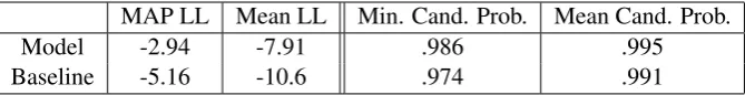
Explaining observed plurals The first test is to show that the model can learn a phonological system for the observed plurals. The model satisfies this goal if it predicts the observed forms at least as well as the baseline model. We calculate both the mean and MAP values of the data likelihood (Eq. 2) over the final 100 iterations of each of the three model runs, and report the across-run means in Table 1. t-tests found no significant differences between the learned and baseline performance on the training data. Predicting novel plurals The second test of the model is whether its learned constraints extend to newly-encountered words. This is a crucial feature for human acquisition; children quickly learn to generalize morphophonological systems. It also represents an important model improvement, as Doyle
4Training words:baby, ball, balloon, banana, bath, bird, blanket, book, car, chair, daddy, diaper, door, drink, eye, hug, key,
kiss, kitty, mommy, nap, nose, phone, shoe, spoon, toothbrush
5There is one deviation from Riggle’s system: we do not specify voicing on sonorants, because sonorants do not have
MAP LL Mean LL Min. Cand. Prob. Mean Cand. Prob.
Model -2.94 -7.91 .986 .995
Baseline -5.16 -10.6 .974 .991
Table 1: Comparing the performance of the learned constraints to the baseline of the standard phono-logical constraint definitions. On the left, training data log-likelihoods on the left, based on values from the final 100 iterations for the three model runs. On the right, test set probability masses for the correct plural forms. The learned constraints perform as well as the phonologically standard constraints.
et al. (2014)’s constraint learning model was incapable of making such predictions due to its strictly-extensional constraints. For the test set, we used the 25 most frequent countable nouns in the Corpus of Contemporary American English (COCA; Davies (2008)) that take regular plurals, none of which were in the training set.6 Five of these nouns end with phonemes that did not occur word-finally in the observed data, requiring the model to have made phonological generalizations from the training data.
To assess the predictive power of the learned constraints, we obtained constraint definitions by us-ing thep(d|m)Metropolis sampler to generate a distribution over definitions for each violation profile. Violation profilesM·l are taken from the final iteration of each model run. For a new candidatey, the
probabilitymy;l thatyviolates constraintlwas estimated using constraintsddrawn from thep(d|M·l)
Metropolis sampler. my;l was then used as the constraint value for the log-linear predictor. Both the
model and baseline constraints correctly put the highest probabilities on the correct plural forms, as shown in Table 1. All correct plural forms received at least98%of the probability mass under the model constraints, and there was no significant difference between the model and baseline predictions.
Violation profile accuracy The previous test showed that the constraint definitions effectively extend to unobserved forms. Now we want to examine their correspondence with phonological theory. First, we want to see if the right number of constraints was learned. Two of the model runs had two marked-ness constraints throughout the final 100 iterations, like the baseline. The third model run used four markedness constraints over its final 100 iterations, but the extra markedness constraints supplied viola-tions that matched two of the faithfulness constraints (DEPand IDENT). Those faithfulness constraints’ weights dropped to near zero in this run, though, meaning that all learning and baseline runs had five active constraints. In the runs with two markedness constraints, we tested how their violation profiles and definitions mapped to the baseline constraints.7 Over the final 100 iterations, the learned violation pro-files agree with their corresponding baseline violation propro-files on an average of98.9%of all candidates, showing that both constraint sets have similar phonological meanings.
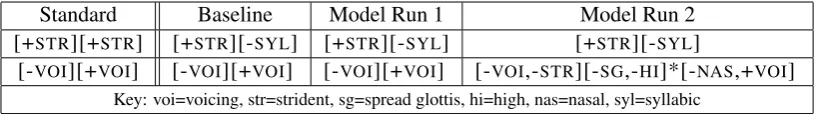
Similarities in constraint definitions We compared the likely constraint definitions, as estimated by the Metropolis sampler forp(d|m), for the learned and baseline violation profiles to their phonologically standard counterparts. Table 2 shows the most likely constraint definitions for each violation profile, given either the baseline violation profiles (based on the standard constraint definitions) and the two-constraint runs of the model. On three of the four learned two-constraints, the model agrees with the inferred definition given the baseline violations. Reasons for the deviations from the phonologically standard definitions are discussed in Sect. 7.
Experiment summary We performed four tests of the constraint learner. The model learned a set of constraints and weights that could explain observed data and effectively generalize to unobserved forms. In addition, we find that the constraint definitions it learns correspond with the definitions that come from a baseline set of constraints, although additional information is needed to identify the exact same constraints as the baseline set.
6These words are: time, year, way, day, thing, world, school, state, family, student, group, country, problem, hand, part,
place, case, week, company, system, program, question, government, number, night
7The remaining analyses are limited to the two-constraint learning runs; the four-constraint solution represents convergence
Standard Baseline Model Run 1 Model Run 2 [+STR][+STR] [+STR][-SYL] [+STR][-SYL] [+STR][-SYL]
[-VOI][+VOI] [-VOI][+VOI] [-VOI][+VOI] [-VOI,-STR][-SG,-HI]*[-NAS,+VOI] Key: voi=voicing, str=strident, sg=spread glottis, hi=high, nas=nasal, syl=syllabic
Table 2: The phonological standard definitions and the most likely constraint definitions inferred in the baseline and model runs. Baseline/modeldlikelihoods based on 10000 samples fromp(d|m).
7 Discussion
Definitional ambiguity Although the constraints extend seamlessly to new data and their violation pro-files mostly match, Table 2 showed the constraint definitions don’t quite match the standard definitions. This is because multiple definitions can have identical violation profiles, as there are many phonological features; for instance, based on the first constraint’s violation profile, the model has learned to penalizesz
andzzsequences, but nots@z. Phonological theory says that this constraint’s definition is [+STR][+STR], but given the available data, any feature that is negative for [z] and [s] but positive for [@] (or vice versa)
will produce the same violation pattern, and the model has no reason to prefer one to the other.8
The complex definition of the second constraint in the second model run arises similarly. Small differ-ences (8%of violations) between the model and baseline violation profiles lead the model to infer this more complicated definition, which penalizes stems ending in voiceless non-stridents getting either the [@z] suffix (with [@] matching the [-SG,-HI] bundle and [z] matching [-NAS,+VOI]) or the [z] suffix (with
the Kleene star vacuously satisfied). Such stems should get the [s] suffix, so this constraint definition is
consistent with the observed data, and overreaching by handling two constraints’ function: penalizing [z] like the [-VOI][+VOI] constraint would, but also penalizing [@z], which is covered by the faithfulness
constraint DEP.
Such definitional ambiguity can be reduced through simultaneous learning of multiple phonological phenomena. The [+STR][-SYL] definition could be ruled out by observing the faithful manifestation of s-initial onset clusters in English, as in stop or spin; the Kleene-star definition could be ruled out
by faithful realizations of non-harmoniouskid orpeg. Such learning would also be more realistic, as learners generally observe and learn a range of phonological phenomena simultaneously.
Relaxing binarity One important remaining step is to allow for non-binary constraints in the model, which could be introduced in multiple ways. One possibility is to mimic non-binary constraints through multiple, overlapping binary constraints (Frank and Satta, 1998), though this would require changes to the current PCFG. Another possibility is to treat the existing binary matrix as an indicator of whether a constraint is violated and add a second matrix, with positive integer values, corresponding to the number of violations of that constraint. Griffiths and Ghahramani (2011) use a similar design to overcome the binary nature of an Indian Buffet Process for object recognition.
Theory testing Our model also represents a way to investigate the plausibility of different theoretical statements of a constraint, casting constraint selection through the lens of model comparison. In addition, if the underlying constraint grammar is varied, this model could be used to investigate the plausibility and effectiveness different potential grammars.
8 Conclusion
We presented a model for learning binary, symbolically-defined constraints in a log-linear model from a combination of observational data and an infinite grammar over constraint definitions. We tested this model on a morphophonological problem and showed that it accurately inferred the values of the con-straints, and found appropriate constraint definitions (though with some issues of definitional ambiguity).
8In fact,p(d|m)is approximately equal for a range of constraint definitions that include [+STR][-SYL], [+STR][+STR],
Acknowledgements
We wish to thank Eric Bakovi´c, Klinton Bicknell, Dave Barner, Charles Elkan, Andy Kehler, the UCSD Computational Psycholinguistics Lab, the Phon Company, and the COLING reviewers for their discus-sions and feedback on this work. This research was supported by NSF award IIS-0830535 and an Alfred P. Sloan Foundation Research Fellowship to RL.
References
Doug Beeferman, Adam Berger, and John Lafferty. 1999. Statistical models for text segmentation. Machine Learning, 34:177–210.
Iris Berent, Colin Wilson, Gary F. Marcus, and Douglas K. Bemis. 2012. On the role of variables in phonology: Remarks on Hayes and Wilson 2008. Linguistic Inquiry, 43:97–119.
Paul Boersma and Bruce Hayes. 2001. Empirical tests of the Gradual Learning Algorithm. Linguistic Inquiry, 32:45–86.
Joan Bresnan, Anna Cueni, Tatiana Nikitina, and R. Harald Baayen. 2007. Predicting the dative alternation. In G. Bourne, I. Kraemer, and J. Zwarts, editors, Cognitive Foundations of Interpretation. Royal Netherlands Academy of Science, Amsterdam.
Philip S. Dale and Larry Fenson. 1996. Lexical development norms for young children. Behavioral Research Methods, Instruments, and Computers, 28:125–127.
Mark Davies. 2008. The Corpus of Contemporary American English: 450 million words, 1990-present.
Gabriel Doyle, Klinton Bicknell, and Roger Levy. 2014. Nonparametric learning of phonological constraints in Optimality Theory. InProceedings of the Association for Computational Linguistics.
Robert Frank and Giorgio Satta. 1998. Optimality theory and the generative complexity of constraint violability. Computational Linguistics, 24:307–315.
Sharon Goldwater and Mark Johnson. 2003. Learning OT constraint rankings using a Maximum Entropy model.
InProceedings of the Workshop on Variation within Optimality Theory.
Noah Goodman, Joshua Tenebaum, Jacob Feldman, and Tom Griffiths. 2008. A rational analysis of rule-based concept learning. Cognitive Science, 32:108–154.
Dilan G¨or¨ur, F. J¨akel, and Carl Rasmussen. 2006. A choice model with infinitely many latent features. In Proceedings of the 23rd International Conference on Machine Learning.
Thomas Griffiths and Zoubin Ghahramani. 2005. Infinite latent feature models and the Indian buffet process. Technical Report 2005-001, Gatsby Computational Neuroscience Unit.
Thomas Griffiths and Zoubin Ghahramani. 2011. The Indian Buffet Process: An introduction and review.Journal of Machine Learning Research, 12:1185–1224.
Bruce Hayes and Colin Wilson. 2008. A maximum entropy model of phonotactics and phonotactic learning. Linguistic Inquiry, 39:379–440.
Bruce Hayes. 1995.Metrical Stress Theory: Principles and Case Studies. U. of Chicago, Chicago.
Bruce Hayes. 1999. Phonetically driven phonology: the role of optimality theory and inductive grounding. In M. Darnell, E. Moravcsik, M. Noonan, F. Newmeyer, & K. Wheatley, editor,Formalism and Functionalism in Linguistics, vol. 1. Benjamins.
John McCarthy. 2008. Doing Optimality Theory. Blackwell.
Radford Neal. 1994. Response to approximate Bayesian inference with the weighted likelihood bootstrap.Journal of the Royal Statistical Society. Series B (Methodological), 56:3–48.
Franz Josef Och and Hermann Ney. 2002. Discriminative training and maximum entropy models for statistical machine translation. InProceedings of the 40th Annual Meeting of the ACL.
Hoifung Poon, Colin Cherry, and Kristina Toutanova. 2009. Unsupervised morphological segmentation with log-linear models. InProceedings of the North American Chapter of the Association for Computational Linguistics. Alan Prince and Paul Smolensky. 1993. Optimality Theory: Constraint interaction in generative grammar.
Tech-nical report, Rutgers Center for Cognitive Science.
Jason Riggle. 2009. Generating contenders.Rutgers Optimality Archive, 1044. Jason Riggle. 2012. Phonological feature chart (v. 12.12). December.