The Complexity of Math Problems – Linguistic, or Computational?
Takuya Matsuzaki1, Hidenao Iwane2, Hirokazu Anai2,3 and Noriko Arai1 1National Institute of Informatics, Japan
2 Fujitsu Laboratories Ltd., Japan 3 Kyushu University, Japan
{takuya-matsuzaki,arai}@nii.ac.jp; {iwane,anai}@jp.fujitsu.com
Abstract
We present a simple, logic-based archi-tecture for solving math problems writ-ten in natural language. A problem is firstly translated to a logical form. It is then rewritten into the input language of a solver algorithm and finally the solver finds an answer. Such a clean decomposi-tion of the task however does not come for free. First, despite its formality, math text still exploits the flexibility of natural lan-guage to convey its complex logical con-tent succinctly. We propose a mechanism to fill the gap between the simple form and the complex meaning while adhering to the principle of compositionality. Second, since the input to the solver is derived by strictly following the text, it may require far more computation than those derived by a human, and may go beyond the capa-bility of the current solvers.
Empirical study on Japanese university en-trance examination problems showed pos-itive results indicating the viability of the approach, which opens up a way towards a true end-to-end problem solving system through the synthesis of the advances in linguistics, NLP, and computer math.
1 Introduction
Development of an NLP system usually starts by decomposing the task into several sub-tasks. Such a modular design is mandatory not only for the reusability of the component technologies and the extensibility of the system, but also for the sound and steady advancement of the research field. Each module, however, has to attack its sub-task in isolation from the entirety of the task, usually with a quite limited form and amount of knowledge. The separated sub-task is hence not
necessarily easy even for human. This problem has been investigated in various directions, includ-ing the solutions to the error-cascadinclud-ing in pipeline models (Finkel et al., 2006; Roth and Yih, 2007, e.g.), the injection of knowledge into the process-ing modules (Koo et al., 2008; Pitler, 2012, e.g.), and the invention of a novel way of modularization (Bangalore and Joshi, 2010, e.g.).
In this paper, we present a simple pipeline archi-tecture for natural language math problem solving, and investigate the issues regarding the separation of the semantic composition mechanism and the mathematical inference. Although the separation between these two may appear to be of different nature than the above-mentioned issues regarding the system modularization, as we will see later, the technical challenges there are also in the tension between the generality of an implemented theory as a reusable component, and its coverage over domain-specific phenomena.
In the system, a problem is analyzed with a Combinatory Categorial Grammar (Steedman, 2001) coupled with a semantic representation based on the Discourse Representation Theory (Kamp and Reyle, 1993) to derive a logical form. The logical form is then rewritten to the input lan-guage of a solver algorithm, such as specialized math algorithms and theorem provers. The solver finally finds an answer through inference.
Natural language problem solving in math and related domain is a classic AI task, which has served as a good test-bed for the integration of various AI technologies (Bobrow, 1964; Charniak, 1968; Gelb, 1971, e.g.). Besides its attraction as a pure intellectual challenge, it has direct applica-tions to the natural language interface for the for-mal systems such as databases, theorem provers, and formal proof checkers. The necessity of the interaction between language understanding and backend solvers has been pointed out in some of the classic works and also in closely related works
terms t::=v|f(t1, . . . , tk)|Λv.t|Λv.D
conditions C::=P(t1, . . . , tk)| ¬D|D1→D2
DRSs D::= ({v1, . . . , vk},{C1, . . . , Cm})
Figure 1: Syntax of DRS
such as Winograd’s SHRDLU (1971). A clear sep-aration of the two layers is, however, an essential property for a wide-coverage problem solving sys-tem since we can extend it in a modular fashion, by the enhancement of the solver or the addition of different types of solvers.
The research question in the current paper is thus summarized as follows:
1. Can we derive the logical form of the prob-lems compositionally, with no intervention of mathematical inference, and how?
2. Can we solve such a direct translation of the text to a logical form with the current state-of-the-art automatic reasoning technology?
After a brief overview of the system pipeline (§3), we present a technique for capturing the dynamic properties of the syntax-semantics mapping in the math problem text, which, at first sight, seem to call for mathematical inference during the deriva-tion of a logical form (§4). We then describe re-maining issues we found so far in the semantic analysis of math problem text (§5). Finally, the viability of the approach is empirically evaluated on real math problems taken from university en-trance examinations. In the evaluation, we apply a solver to the logical forms derived through manu-ally annotated CCG derivations and DRSs on the problem text (§6). In the current paper, we thus exclusively focus on the formal aspect of the se-mantic analysis, setting aside the problem of its automation and disambiguation. The final section concludes the paper and gives future prospects in-cluding the automatic processing of the math text.
2 Preliminaries
2.1 Discourse Representation Structure
We use a variant of Discourse Representation Structure (DRS) (Kamp and Reyle, 1993) for the semantic representation. DRS has been developed for the formal analysis of various discourse phe-nomena, such as anaphora and quantifier scopes beyond a single sentence.
Fig. 1 shows the syntax of DRS used in this paper.1 In the definitions, f and P respectively denote a function and a predicate symbol and v
denotes a variable. The definition is slightly ex-tended from that by van Eijck and Kamp (2011) for incorporating higher-order terms. A term of the formΛv.M denotes lambda abstraction in the object language, which is used to represent (math-ematical) functions and sets2; we reserveλfor de-noting the abstraction over DRSs (and terms) for the composition of DRSs. We define the interpre-tation of a DRSDindirectly through its translation
D◦to a (higher-order) predicate logic as in Fig. 2. As defined in Fig. 2, a DRS D = (V,C) is basically interpreted as a conjunction of the con-ditions inCthat is quantified existentially by all the variables in V. However, as in the second clause in Fig. 2, the variables in the antecedent of an implication are universally quantified and their scopes also cover the succedent; this definition is utilized in the analysis of sentences including in-definite NPs, such as donkey sentences.
The mechanism of the DRS composition in this paper is based on the formulation by van Eijck and Kamp (2011). They use an operation called merge (denoted by•) to combine two DRSs. Assuming no conflicts of variable names, it can be defined as:(V1,C1)•(V2,C2) := (V1∪V2,C1∪C2).
Roughly speaking, this operation amounts to form the conjunction of the conditions in C1 and C2
allowing the conditions inC2 to refer to the
vari-ables inV1. Consider the following discourse:
s1: A monkeyxis sleeping. s2: Itxholds a banana.
Assuming the anaphoric relation indicated by the super/sub-scripts, we have their DRSs as follows:
D1= ({x},{monkey(x),sleep(x)})
D2 = ({y},{banana(y),hold(x, y)})
By merging them, we have
D1•D2 =
( {x, y},
{
monkey(x),sleep(x),
banana(y),hold(x, y)
})
,
which is translated to∃x.∃y.(monkey(x)∧ · · · ∧ hold(x, y))as expected.
1
Disjunction can be defined by using implication and negation:D1∨D2 := ({},{¬D1})→D2.
2We represent the application of aΛ-term to another term,
such as(Λx.D)tand(Λx.t1)t2, either by a special predicate
App(f, x)≡ f xor a functionapp(f, x) := f xaccording to the type off. Compound terms of the formt1t2are hence
Assuming D1= ({v1, . . . , vk},{C1, . . . , Cm}),
D1◦:=∃v1. . .∃vk.(C1◦∧ · · · ∧Ck◦)
(D1→D2)◦:=∀v1. . .∀vk.((C◦1∧ · · · ∧Cm◦)→D◦2)
(¬D)◦:=¬D◦
(P(t1, t2, . . .))◦:=P(t◦1, t◦2, . . .)
(f(t1, t2, . . .))◦:=f(t◦1, t◦2, . . .)
(Λv.D)◦:= Λv.(D◦)
(Λv.t)◦:= Λv.(t◦)
v◦:=v
Figure 2: Translation of DRS to HOPL
When
S/S/S :λP.λQ.P→Q
the centers ofC1andC2
S/(S\NP)
:λP.({x, x1, x2},{x= [x1, x2], x1= center of(C1), x2= center of(C2)})•P x
coincide
S\NP :λx.({},{coincide(x)}) >
S: ({x, x1, x2},{x= [x1, x2], x1= center of(C1), x2= center of(C2),coincide(x)})
>
S/S:λQ.({x, x1, x2},{x= [x1, x2], x1= center of(C1), x2= center of(C2),coincide(x)})→Q
Figure 3: A part of CCG derivation tree
X/Y :f Y :a >
X:f a
X/Y :f Y /Z:g >B
X/Z:λx.f(gx)
Figure 4: Example of combinatory rules
2.2 Combinatory Categorial Grammar
Combinatory Categorial Grammar (CCG) (Steed-man, 2001) is a lexicalized grammar formalism. In CCG, the association between a wordwand its syntactic/semantic property is specified by a lexi-cal entry of the formw := C :S, whereCis the category ofwandSis the semantic interpretation ofw. A category is either a basic category (e.g., S,N,NP) or a complex category of the formX/Y
orX\Y. For instance, we can assign the follow-ing categories and semantic interpretations to the region notation “[0,+∞)” and a bare noun phrase “positive number”:
[0,+∞) := NP: Λx.({},{x≥0})
positive number := N:λx.({},{x >0})
since the region notation behaves as a proper noun and it can be represented by its characteristic func-tion, while “positive number” functions like a common noun (recall thatΛ is for the abstraction in the object language andλstands for the abstrac-tion for the DRS composiabstrac-tion). A handful of com-binatory rules define how the categories and the semantic interpretations of constituents are com-bined to derive a larger phrase. Fig. 4 shows two of the rules. A part of a derivation tree for “When the centers of C1 and C2 coincide” is shown in
Fig. 3. As shown in the figure, the semantic repre-sentation in DRS is composed by the beta reduc-tion and the DRS merge operareduc-tion. As we will see in§4, there are certain types of discourse for which the basic DRS composition machinery de-scribed so far does not suffice. We will return to this after a brief description of the whole system.
3 A Simple Pipeline for Natural Language Math Problem Solving
The main result in the current paper is a mech-anism of semantic composition and an empirical support for our overall design choice. Although the NLP modules for the automatic processing and disambiguation are still under development, we show a brief overview of the whole system to give a clear image on the different representations of a problem at different stages of the pipeline.
From text to logical form The system receives a problem text with LATEX-style markup on the
symbolic mathematical expressions: e.g.,
Let $a>0$, $b≤0$, and $0<p<1$. $P(p, pˆ2)$ is on the graph of the function$y=ax-bxˆ2$. Write$b$in terms of$a$and$p$.
We process the mathematical expressions with a symbolic expression analyzer and produce their possible interpretations as lexical entries. For in-stance,$y=ax-bxˆ2$in the above example will receive at least two interpretations:
$y=ax-bxˆ2$ := S: ({},{y=ax−bx2})
$y=ax-bxˆ2$ := NP: Λx.ax−bx2.
The first lexical entry is for the usages such as “Hencey =ax−bx2,” where the expression de-notes a proposition and behaves as a sentence. The second entry is for the usage as a noun phrase as in the example, which stands for a function.
language we’ll introduce in the next section):
D1 = ({},{a >0, b≤0,0< p, p <1}) D2 = ({},{P = (p, p2),on(P,Λx.ax−bx2)}) D3 = Find(b′)
[
cc;∃−1a;∃−1p;b=b′]
A discourse structure analyzer receives the DRSs and determines the logical relations among them while selecting an antecedent for each anaphoric expression. The net result of this stage is a large DRS that represents the whole problem. For the above example, we have their sequencing as the result: D1;D2;D3. The sequencing
opera-tor (;) basically means conjunction (merge) of the DRSs, but it is also used to connect the meanings of a declarative sentence and an imperative sen-tence. The large DRS is then translated by a pro-cess defined in the next section, giving a HOPL formula enclosed by a directive to the solver:
Find(b′)
[
a >0∧b≤0∧0< p∧p <1∧
∃P. (
P = (p, p2)∧
on(P,Λx.ax−bx2)∧ b=b′ ) ]
,
whereFind(v)[ϕ]is a directive to find the value of variablevthat satisfies the conditionϕ.
From logical form to solver input Many of the current automatic reasoners operate on first-order formulas. To utilize them, we hence have to trans-form the HOPL trans-formula in a directive to an equiv-alent first-order formula. Such transformation is of course not possible in general. However, we found that a greedy rewriting procedure suffices for that purpose on all of the high-school level math prob-lems used in the experiment.
In the rewriting procedure, we iteratively ap-ply several equivalence-preserving transforma-tions including the beta-reduction ofΛ-terms and rewriting of the predicates and functions using their definitions. For the above example, by us-ing some trivial simplifications and the definition ofon(·,·):
∀x.∀y.∀f.(on((x, y), f)↔(y=f x)),
we have the following directive holding a first-order formula:
Find(b′)
[
a >0∧b≤0∧0< p∧p <1∧
p2=ap−bp2∧b=b′
]
.
Solver Algorithms In addition to the generic first-order theorem provers, we can use specific algorithms as the solver when the formula is ex-pressible in certain theories. Among them, many
mathematical and engineering problems can be naturally translated to formulas consisting of poly-nomial equations, inequalities, quantifiers (∀,∃) and boolean operators (∧,∨,¬,→, etc). Such for-mulas construct sentences in the first-order theory of real closed fields (RCF).
In his celebrated work, Tarski (1951) showed that RCF allows quantifier-elimination (QE): for any RCF formula ϕ(x1, . . . , xn), there exists an equivalent quantifier-free formula ψ(x1, . . . , xn) in the same vocabulary. For example, the for-mula ∃x.(x2 +ax+b ≤ c) can be reduced to a quantifier-free formulaa2−4b+ 4c≥0by QE. Automated theorem proving is usually very costly. For example, QE for RCF is doubly ex-ponential on the number of quantifier alternations in the input formula. The problems containing only six variables may be hard for today’s com-puter with the best algorithm known. However, several positive results have been attained as the result of extensive search for practical algorithms during the last decades (see (Caviness and John-son, 1998)). Efficient software systems of QE have been developed on several computer algebra systems, such asSyNRAC(Iwane et al., 2013).
4 Formal Analysis of Math Problem Text
In this section, we first summarize the most promi-nent issues we found so far in the linguistic analy-sis of high-school/college level math problems and then present a solution.
4.1 Problems
Context-dependent meanings of superlatives and their alike The meaning of a superla-tives and semantically similar expressions such as “maximum” generally depends highly on the con-text. For example, the interpretation of “John was the tallest” depends on the group (of people) that is prominent in the discourse:
There were ten boys. John was the tallest.
This context-dependency can be made more ex-plicit by paraphrasing it to a comparative (Heim, 2000): “John was taller thananyone else,” where “anyone else” refers, depending on the context, to the group against which John was compared.
In math text, however, we can usually determine the range of the “anyone else” without ambiguity:
Here, the set of values that should be compared against the maximum value is, with no ambiguity, all the possible values ofabthat is determined by the preceding context. Once we have a represen-tation of such a set, it is easy to write the seman-tic interpretation of the phrase “maximum value ofα.” But, how can we obtain a representation of such a set without inference?
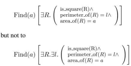
Discrimination between free/bound variable
We can explicitly specify that a variable should be interpreted as being free, as in:
Let R be a square with perimeter l. Write the area ofRin terms ofl.
This discourse may be translated to
Find(a)
[ ∃R.
(
is square(R)∧ perimeter of(R) =l∧
area of(R) =a
)]
but not to
Find(a)
[ ∃R.∃l.
(
is square(R)∧ perimeter of(R) =l∧
area of(R) =a
)]
since, assuming the proper definitions of the func-tions and predicates, the first one is equivalent to
Find(a)[a = l2/16]but the second one is
equiv-alent to Find(a)[a > 0]. How can we specify a variable benotbound?
Imperatives Math problems usually in-clude imperatives such as “Find/Write...,” and “Prove/Show...”. How can we derive correct in-terpretations of those imperatives, which depend on the semantic content of preceding declarative sentences, but are not a part of the declarative meaning of a discourse?
4.2 Solution by iDRS
Although the above-mentioned phenomena are quite common in math problem text, we found it is difficult to derive the meanings of such expres-sions within the basic compositional DRS frame-work introduced in§2. All of the examples above involve the manipulation and modification of the context in a discourse.
We present an extension of the DRS composi-tion mechanism that covers expressions like the above examples. The basic idea is to introduce an-other layer of semantic representation called iDRS hereafter, which provides a device to manipulate
terms t::=v|f(t1, . . . , tk)|Λv.t|Λv.I
iDRS I::=P(t1, . . . , tk)| ¬I|I1→I2|
[image:5.595.71.290.285.396.2]∃v|I1;I2| ∃−1v|Find(v)[I]|Show[I]|cc
Figure 5: Syntax of iDRS
the representation of the preceding context during the semantic composition.3
First we define the syntax of iDRS as in Fig. 5. In the definition, the variables P, f, t, and v fol-lows the same convention as in the DRS definition. In words, an iDRS represents either a DRS condi-tion (the first row of the definicondi-tion ofI), a quan-tification∃v, which corresponds to a DRS having only one variable, ({v},{}), a sequencing I1;I2
of two iDRSs, or the new ingredients in the rest of the definition that will be explained shortly.
The “anti-quantifier”∃−1v means an operation that cancels the quantification onv that precedes
∃−1v. Find(v)[I] is a directive that requires to
find the set of the values of variablev which sat-isfy the condition represented by I. Similarly,
Show[I] is a directive that requires to prove the statement represented byI. Note that these two di-rectives are not specific to any solvers; The choice of the solver depends on the theory (e.g., RCF) under which the formula in a directive is under-stood. The last element, cc, can be considered as a special ‘variable’, through which we can always retrieve an iDRS representation of the context that precedes the position marked by thecc.
Using these new ingredients, we can now write, for instance, the semantic representation of the phrase “maximum value” as follows:
N/NPof :λx.λm.max(Λy.(cc;y=x), m),
assuming that the two-place predicate max(s, m) is defined to be true iff m is the maximum ele-ment in the set s (represented by a Λ-term). A sentence “the maximum value ofxism” will thus havemax(Λy.(cc;y=x), m)as its semantic rep-resentation, which means thatmis the maximum value ofxthat satisfies the condition specified by the preceding context.
3
{{I1;I2}}c := {{I1}}c;{{I2}}c;[[I1]]c {{Find(v)[I]}}c := Find(v) [[[I]]c]
{{Show[I]}}c := Show [[[I]]c] {{I1 →I2}}c := {{I2}}c;[[I1]]c
{{I}}c := ϵ
[[cc;I]]c := c; [[I]]c
[[cc]]c := c
[[I1;I2]]c := [[I1]]c; [[I2]]c;[[I1]]c
[[I1→I2]]c := [[I1]]c→[[I2]]c;[[I1]]c
[[¬I]]c := ¬[[I]]c
[[Find(v)[I]]]c := ∃v; [[I]]c
[[Show[I]]]c := [[I]]c
[[P(t1, . . .)]]c := P([[t1]]c, . . .)
[[∃v]]c := ∃v
[[∃−1v]]c := ∃−1v
[[v]]c := v
[[f(t1, . . .)]]c := f([[t1]]c, . . .)
[[Λv.t]]c := Λv.[[t]]c
[image:6.595.83.526.70.161.2][[Λv.I]]c := Λv.[[I]]c
Figure 6: Transformation from iDRS to directive sequence
Let’s take the following problem as an example:
Let p > 0. R is a rectangle whose perimeter isp. Find the maximum value of the area ofRas a function ofp.
We have its iDRS representation shown below, by parsing the sentences and composing the resulting iDRSs into one (in this case, just by sequencing the three sentences’ iDRSs):
0< p;
is rectangle(R); perimeter of(R) =p;
∃m; max(Λx.[cc;x= area of(R)], m); Find(a)[cc;∃−1p;a=m]
We then bind all free variables in the iDRS at their narrowest scopes:
∃p; 0< p;
∃R; is rectangle(R); perimeter of(R) =p;
∃m; max(Λx.[cc;x= area of(R)], m); Find(a)[cc;∃−1p;a=m]
This amounts to assume each variable appearing in a problem text is, unless it is explicitly quantified, interpreted to be existentially quantified as default, and to be universally quantified if it appears in the antecedent of an implication.
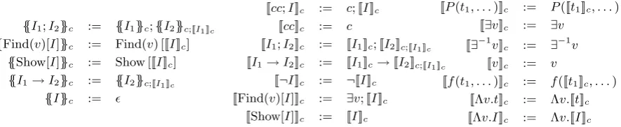
The iDRS is then processed by the functions
{{·}}c and [[·]]c defined in Fig. 6. In the defini-tion, ϵstands for an empty sequence. The func-tion{{·}}cextracts the imperative meaning from an iDRS, using[[·]]cas a ‘sub-routine’ that extracts the declarative meaning from an iDRS. The suffix (c) of the two functions stands for the preceding con-text represented as an iDRS. When[[·]]cprocesses a sequenceI1;I2 or an implication I1 → I2, the
declarative content ofI1 (i.e.,[[I1]]c) is appended to the preceding contextc, andc; [[I1]]cis passed as the preceding context when processing I2. When
[[·]]c finds acc variable, it substitutes the cc with the current context stored in the suffix.
By applying{{·}}ϵto the iDRS of a problem, we can extract the logical form of the problem as a
sequence of directives. For the example problem, we have a single directive as follows:
Find(a)
∃p; 0< p;
∃R; is rectangle(R); perimeter of(R) =p;
∃m; max(Λx.
∃p; 0< p;
∃R; is rectangle(R); perimeter of(R) =p;
∃m;x= area of(R)
, m);
∃−1p;a=m
Now, by the definition of{{·}}cand[[·]]c, the iDRSI inside a directiveFind(v)[I]orShow[I]includes only those elements that have a counterpart in the basic DRS except for the “anti-quantifiers.” We can hence convert it to a HOPL formula, by first canceling the quantifications∃vthat precede∃−1v
(i.e., deleting all occurrences of∃vthat appear be-fore an occurrence of∃−1vin the iDRS, and delet-ing ∃−1v itself), then converting it to a DRS by replacing the sequencing operator ‘;’ to the merge operator, and finally translating it to a HOPL for-mula according to Fig. 2.
5 Remaining Issues in the Semantic Analysis of Math Problem Text
The mechanism presented in §4 significantly en-hanced the coverage of the analysis over real prob-lems. We however found several phenomena that can not be handled now.
Free/bound variable distinction without a cue phrase We have presented a mechanism to ‘un-bind’ the variables specified by a cue phrase, such as “(findx) in terms of (y).” Some types of vari-ables however have to be left free even without any explicit indication, e.g.:
Letp >0. Find the area of a circle with radiusp, centered at the origin.
Assumingcircle(x, y, r) denotes a circle with ra-diusrand centered at(x, y), we want to derive
but our default variable binding rule gives
Find(a) [∃p;p >0;a= area of(circle(0,0, p))].
This directive means to find the range of the areas of the circles with arbitrary radii, which is appar-ently not a possible reading of the problem. We found such cases in 3 out of the 32 test problems used in the experiment shown later.
Scope inversion by a cue phrase The hierar-chy of the quantifier scopes in math text mostly follows the linear order of the appearance of the variables (either overtly quantified or not). This general rule can however be superseded by the effect of a cue phrase, as shown in the example problem and its possible translation in Fig. 7. In the figure, the formula inside the Show-directive mostly follows the discourse structure, in that the predicates from the first and the second sentence respectively form the antecedent and the succe-dent of the implication. The quantification on F
is however dislocated from its default scope, i.e., the succedent, and moved to the outset of the for-mula by the effect of the underlined cue phrases. To handle such cases correctly, we would need a more involved mechanism for the manipulation of the context representation through theccvariable.
Idiomatic expressions As in other text genres, idiomatic multiword expressions are also prob-lematic as can be seen in the following example:
By choosing x sufficiently large, y = 1/xcan be made as close to 0 as desired.
As the example shows, a set phrase involving com-plex syntactic relations, e.g., “can do X as Y as desired by choosing Z sufficiently W” and “X ap-proaches Y as Z apap-proaches W,” can convey id-iomatic meanings in math.
6 Empirical Results
We tested the feasibility of our approach on a set of problems selected from Japanese university en-trance exams. Specifically, we wanted 1) to test the coverage of the semantic composition mecha-nism presented in §4 on real problems, and 2) to verify that there is no significant loss in the capa-bility of the system due to the additional compu-tational cost incurred by the separation of the se-mantic analysis from the mathematical reasoning. The second point was confirmed by provid-ing the ideal (100% correct) output from the
(forthcoming) NLP components to a state-of-the-art automatic reasoner and comparing the result against the performance of the reasoner on the input formulated by a human expert. Specifi-cally, we manually gave the semantic representa-tions of the problems as iDRSs or CCG deriva-tion trees, and then automatically rewrote them into the language of RCF. The resulting formu-las were fed to a solver to see whether the an-swers be returned in a realistic amount of time (30 seconds). The solver was implemented on SyN-RAC (Iwane et al., 2013), which is an RCF-QE solver implemented as an add-on to Maple, and the (in)equation solving commands of Maple.
The problems were taken from the entrance ex-ams of five first-tier universities in Japan (Tokyo U., Kyoto U., Osaka U., Kyushu U., and Hokkaido U.) for fiscal year 2001, 2003, 2005, 2007, 2009 and 2011. There were 249 problems in total. From them, we first eliminated those that included al-most no natural language text, such like calcula-tion problems. We then chose, from the remaining non-straightforward word problems, all the prob-lems which could be solved with SyNRAC and Maple when the input was formulated by an expert of computer algebra. The formulation by an expert was done, of course, with no manual calculation, but otherwise it was freely done including the di-vision of the solving process into several steps of QE and (in)equation solving.
As the result of that, we got 32 test problems, each of which contained 3.9 sentences on aver-age. They include problems on algebra (of real and complex numbers), 3D and 2D geometry, cal-culus, and their combinations. For analyzing the result in more detail, we divided the problems into 78 sub-problems for which the correctness of the answers can be judged independently.
6.1 From discourse analysis to the solution
Problem: PointP is on the circlex2+y2 = 4andl
P is the normal line to the circle atP. Show thatlP passes through a fixed pointFirrespective ofP.
Show
[
∃F. (
∀P.∀lP.
((
P is onx2+y2= 4and
lPis the normal line to the circle atP
)
→lP passes throughF
))]
Figure 7: Scope inversion by cue phrases
LetO(0,0),A(2,6),B(3,4)be 3 points on the coordi-nate plane. Draw the perpendicular to lineABthrough
O, which meetsAB atC. Lets, tbe real numbers, and letP be such thatOP =s−→OA+t−−→OB. Answer the following questions.
(1) Calculate the coordinates of point C, and write |−−→CP|2in terms ofsandt.
(2) Letsbe constant, and lettvary in the ranget≥0. Calculate the minimum of|−−→CP|2.
Figure 8: Kyushu University 2009 (Science Course) Problem 1
composed from word-level semantic representa-tions. In the iDRS encoding of the 32 problems, the context-fetching mechanism through ‘cc’ vari-able was needed in 15 problems and the canceling of quantification was needed in 6 problems. These mechanisms thus significantly enhanced the cov-erage of the semantic composition machinery.
After rewriting the iDRSs to RCF formulas4, we fed them to the solver and got perfect answers for 19 out of the 32 problems. Out of the 78 sub-problems, 56 sub-problems (72%) were success-fully solved. 12% of the problems (9 sub-problems) failed due to the timeout in the QE solver. Besides the timeout, a major cause of the failures (7 sub-problems) was the fractional power (mainly square root) in the formula. Although we can mechanically erase the fractional powers to get an RCF formula, it was not implemented in the solver.5 The remaining 6 sub-problems needed the free/bound variable distinction with-out any cue phrase (§5). Although half of them could be solved by manually specifying the free variables, we did not count them as solved here.
6.2 From syntactic analysis to the answer
We chose 14 problems from the 19 problems which were fully solved with the iDRS
encod-4
The knowledge-base used to rewrite the HOPL formu-las to first-order RCF formuformu-las included 230 axioms for 86 predicates and 98 functions.
5In the formulation by the human expert, the use of square
roots were avoided by encoding the conditions differently (e.g.,x≥0∧x2= 2instead of√x= 2).
ings. We manually analyzed the text following the CCG-based analyses of basic Japanese construc-tions given by Bekki (2010). We annotated the 44 sentences in the 14 problems with full CCG derivation trees and anaphoric links. We selected the 14 problems so that they cover different types of grammatical phenomena as much as possible. The final CCG lexicon contained 240 lexical en-tries (109 for function words and the rest for con-tent words). The iDRS representations were then derived by (automatically) composing the seman-tic representations of the words according to the derivation trees and combining the sentence-level iDRSs to a problem-level iDRS as in the first ex-periment. Out of the 14 problems, we got fully correct answers for 13 problems. In the 14 prob-lems, there were 33 sub-problems and we got cor-rect answers for 32 of them; On only one sub-problem, the solver could not return an answer within the time limit. Fig. 8 shows an English translation of one of the 13 problems successfully solved with the CCG derivation trees as the input. Overall, the results on the real exam problems were very promising: 72% of the sub-problems were successfully solved with the formula derived from a sentence-by-sentence, direct encoding of the problem. The experiment with manually an-notated CCG derivation trees further showed that there was almost no additional cost introduced by the mechanical derivation of the logical forms from the word-level semantic representations.
7 Conclusion and Prospects
References
Srinivas Bangalore and Aravind K. Joshi. 2010. Su-pertagging: Using Complex Lexical Descriptions in Natural Language Processing. Bradford Books. MIT Press.
Daisuke Bekki. 2000. Typed Dynamic Logic for Com-positional Grammar. Ph.D. thesis, University of Tokyo.
Daisuke Bekki. 2010. Formal Theory of Japanese Syn-tax. Kuroshio Shuppan. (In Japanese).
Daniel Gureasko Bobrow. 1964. Natural language in-put for a comin-puter problem solving system. Ph.D. thesis, Massachusetts Institute of Technology.
Adrian Brasoveanu. 2012. The grammar of quantifica-tion and the fine structure of interpretaquantifica-tion contexts. Synthese, pages 1–51.
Bob F. Caviness and Jeremy R. Johnson, editors. 1998. Quantifier Elimination and Cylindrical Algebraic Decomposition. Springer-Verlag, New York.
Eugene Charniak. 1968. Carps: a program which solves calculus word problems. Technical report, Massachusetts Institute of Technology.
Jenny Rose Finkel, Christopher D. Manning, and An-drew Y. Ng. 2006. Solving the problem of cascad-ing errors: approximate bayesian inference for lin-guistic annotation pipelines. InProceedings of the 2006 Conference on Empirical Methods in Natural Language Processing, EMNLP ’06, pages 618–626, Stroudsburg, PA, USA. Association for Computa-tional Linguistics.
Jack P. Gelb. 1971. Experiments with a natural lan-guage problem-solving system. InProceedings of the 2nd international joint conference on Artificial intelligence, IJCAI’71, pages 455–462, San Fran-cisco, CA, USA. Morgan Kaufmann Publishers Inc.
Irene Heim. 2000. Degree operators and scope. In Proceedings of Semantics and Linguistic Theory 10, pages 40–64. CLC Publications.
Hidenao Iwane, Hitoshi Yanami, Hirokazu Anai, and Kazuhiro Yokoyama. 2013. An effective implemen-tation of symbolic-numeric cylindrical algebraic de-composition for quantifier elimination. Theoretical Computer Science. (in press).
Hans Kamp and Uwe Reyle. 1993. From Discourse to Logic: Introduction to Modeltheoretic Semantics of Natural Language, Formal Logic and Discourse Representation Theory. Studies in Linguistics and Philosophy. Kluwer Academic.
Terry Koo, Xavier Carreras, and Michael Collins. 2008. Simple semi-supervised dependency parsing. In Proceedings of ACL-08: HLT, pages 595–603, Columbus, Ohio, June. Association for Computa-tional Linguistics.
Emily Pitler. 2012. Attacking parsing bottlenecks with unlabeled data and relevant factorizations. In Pro-ceedings of the 50th Annual Meeting of the Associa-tion for ComputaAssocia-tional Linguistics (Volume 1: Long Papers), pages 768–776, Jeju Island, Korea, July. Association for Computational Linguistics.
Dan Roth and Wen-tau Yih. 2007. Global inference for entity and relation identification via a linear pro-gramming formulation. In Lise Getoor and Ben Taskar, editors,Introduction to Statistical Relational Learning. MIT Press.
Mark Steedman. 2001. The Syntactic Process. Brad-ford Books. MIT Press.
Alfred Tarski. 1951. A Decision Method for Elemen-tary Algebra and Geometry. University of Califor-nia Press, Berkeley.
Jan van Eijck and Hans Kamp. 2011. Discourse rep-resentation in context. In Johan van Benthem and Alice ter Meulen, editors, Handbook of Logic and Language, Second Edition, pages 181–252. Elsevier.