Phonon Anharmonicity of Ionic Compounds and Metals

Metals

Thesis by

Chen W. Li

In Partial Fulfillment of the Requirements for the Degree of

Doctor of Philosophy

California Institute of Technology Pasadena, California

2012

To my lovely wife, Jun, whose support is indispensable through the years,

and

Acknowledgments

First and foremost, I would like to thank my advisor, Brent Fultz, for his guidance and support throughout my graduate student years at Caltech, and especially for his efforts to offer me a second chance at admission after the visa difficulty. I am very fortunate to have had him as a mentor and collaborator during these years. Without his insightful advice, this work would not have been possible.

I owe many thanks to all current and former members of the Fultz group, who have been a constant source of thoughts and support. In particular, I would like to thank Mike McKerns for his guidance on the Raman and computational work. Special thanks to my officemates, Olivier Delaire (now at Oak Ridge National Lab), Max Kresch (now at IDA), Mike Winterrose (now at MIT Lincoln Lab), and Jorge Muñoz, who made the work much more enjoyable. Thanks to the former DANSE postdocs: Nikolay Markovskiy, Xiaoli Tang, Alexander Dementsov, and J. Brandon Keith. You helped me a lot on programming and calculations. Also thanks to other former group members: Matthew Lucas (now at Air Force Research Laboratory), Rebecca Stevens, Hongjin Tan (now at Contour Energy Systems), and Justin Purewal (now at Ford Motor/University of Michigan); as well as other current group members: Hillary Smith, Tian Lan, Lisa Mauger, Sally Tracy, Nick Stadie, and David Abrecht. It is fun to work and travel with you. I would like to extend my special thanks to Jiao Lin for his relentless help on computation matters, and Channing Ahn for his help on experiments using his expertise. I also wish current and future members of the Fultz group the best of luck and hope you to continue to make the group an exciting and fruitful place to work in.

helped me over the years: especially, Bill Johnson and other people in his group, for his illuminating thermodynamics lectures, and sharing their equipment; Mike Vondrus, for his help on building the weird things I designed, and fixing the things I had trouble with; Pam Albertson and many other former Materials Science staff, for their efforts to keep everything running; Avalon Johnson, for keeping the group cluster, where I did most of my work here, up and running.

I wish to acknowledge the generous help and support of our collaborators at Oak Ridge National Laboratory: Doug Abernathy, Matthew Stone, Mark Loguillo, and Matthew Lucas (again), as well as Lee Robertson, Karol Marty, and Mark Lums-den, among many others. They made our inelastic neutron scattering experiments possible through their unrelenting support during many sleepless nights, and were always willing to share their deep knowledge and understanding of neutron scattering.

I wish to take this opportunity to also thank several people in the neutron scattering community for their advice and help on my career: Rob McQueeney, Guangyong Xu, Genda Gu, and Ben Larson.

Finally, I wish to express my gratitude to my parents and my wife, Jun, for their unconditional love and support through the years. It is your encouragement and understanding that kept me up in the darkest days: I would not have made it without you. And Derek, you brought us the paramount joy.

Abstract

Vibrational studies of materials at elevated temperatures are relatively rare, and most phonon work also has emphasized harmonic behavior. Non-harmonic effects are often unexplored. These non-harmonic effects can be important for many properties of the material, such as thermal transport and phase stability.

Phonon theory and computational methods are briefly reviewed, and the exper-imental techniques for phonon study, such as Raman spectroscopy and inelastic neutron scattering, are discussed. Several experiments on phonon anharmonicity were performed, and interpreted with these computational methods.

In Raman spectroscopy studies on the phonon dynamics of hafnia and zirconia, Raman line positions, and shapes of temperatures to 1000 K were measured and the types of modes that exhibit the most anharmonicity were characterized and correlated to the vibrational displacements of individual atoms in the unit cell. It was found that anharmonicity in these systems is rich in information and strongly mode dependent.

Using time-of-flight inelastic neutron scattering, we found purely quartic transverse modes with an anomalous mode stiffening with temperature, and related these modes to the enormous negative thermal expansion of the DO9

structure of scandium fluoride.

Contents

Acknowledgments iv

Abstract vi

List of Figures xiii

List of Tables xvi

I

Introduction

1

1 Introduction 2

1.1 Motivations . . . 3

1.2 Present Work . . . 3

II

Theory

6

2.2 Crystal Lattice . . . 9

2.3 Normal Modes . . . 11

2.4 Phonon Thermodynamics . . . 12

2.5 Temperature Effects . . . 17

2.5.1 Harmonic Phonons . . . 17

2.5.2 Quasiharmonic Thermodynamics . . . 18

2.5.4 Phonon Entropy . . . 21

2.5.5 Electronic Entropy . . . 23

2.6 Lattice Dynamics . . . 24

2.6.1 Interatomic Force-Constants . . . 24

2.6.2 Equations of Motion. . . 26

2.6.3 The Eigenvalue Problem of the Phonon Modes . . . 27

2.6.4 The Phonon Density of States . . . 29

2.6.5 Group Theory . . . 30

2.7 Phonon-Phonon Interactions. . . 30

2.8 Electron-Phonon Interactions . . . 33

3 Computational Techniques 38 3.1 Introduction. . . 39

3.2 First-Principle Methods . . . 39

3.2.1 Many-Body Problem . . . 39

3.2.2 Hartree-Fock Method . . . 40

3.2.3 Variational Principle and Self-Consistent Field Method . . . . 41

3.3 Density Functional Theory . . . 42

3.3.1 Hohenberg-Kohn Theorems . . . 42

3.3.2 Kohn-Sham Theory . . . 43

3.3.3 Exchange and Correlation . . . 44

3.3.4 Choice of Basis Sets and Pseudopotentials . . . 46

3.3.5 More on DFT . . . 47

3.4 Molecular Dynamics (MD) . . . 48

3.4.1 Principles . . . 48

3.4.2 Potentials . . . 50

3.4.3 Solving Equations of Motion. . . 52

3.4.4 Initial Conditions . . . 53

3.4.5 Ensembles and Thermostats . . . 54

3.4.7 More on MD . . . 58

3.5 Packages . . . 59

3.5.1 DFT Codes . . . 59

3.5.2 Classical Lattice Dynamics Codes . . . 60

3.5.3 Phonon Lattice Dynamics Codes . . . 60

III

Scattering Experiment

61

4.2 Scattering Theory . . . 66

4.2.1 Scattering Cross Section . . . 66

4.2.2 Fermi’s Golden Rule . . . 67

4.2.3 Scattering by Crystal . . . 69

4.2.4 Scattering by Phonons . . . 70

4.3 Time-of-Flight Neutron Chopper Spectrometer . . . 73

4.3.1 Concept and Setup . . . 73

4.3.2 Kinematic Limit . . . 75

4.3.3 Time-of-Flight Chopper Spectrometers at the SNS . . . 77

4.3.4 Data Reduction toS(Q, E) . . . 79

4.3.5 Reduction to Phonon DOS . . . 82

4.3.6 Other Considerations . . . 84

4.4 Triple-Axis Neutron Spectrometer . . . 86

4.4.1 Concept and Setup . . . 86

4.4.2 Resolution and Data Reduction . . . 88

4.4.3 Other Considerations . . . 92

4.5 Sample Environments . . . 93

5 Raman Spectroscopy 97 5.1 Introduction. . . 98

5.2.1 Classical Model . . . 100

5.2.2 Quantum Mechanical Model . . . 106

5.2.3 Selection Rules . . . 108

5.2.4 Enhanced Raman . . . 109

5.3 Experimental Techniques. . . 111

5.3.1 Basic Setup . . . 111

5.3.1.1 Lasers . . . 111

5.3.1.2 Spectrometers and Filters . . . 114

5.3.1.3 Detectors . . . 116

5.3.2 Signal-to-Noise Ratio . . . 116

5.3.2.1 Signal . . . 116

5.3.2.2 Noise . . . 118

5.3.3 Geometry . . . 118

5.3.4 Calibration . . . 120

5.3.5 Sample Environments . . . 121

5.4 Data Analysis . . . 123

5.5 Time-Resolved Raman Spectroscopy. . . 123

5.6 Other Raman Techniques . . . 124

5.7 Other Considerations . . . 126

IV

Ionic Compounds

127

6.2 Experiment . . . 132

6.3 Results . . . 134

6.4 Calculations . . . 136

6.5 Discussion . . . 138

7 Zirconium(IV) Oxide (Zirconia, ZrO2) 146

7.1 Introduction. . . 147

7.2 Experiment . . . 150

7.3 Results . . . 150

7.4 Calculations . . . 152

7.5 Discussion . . . 156

7.6 Conclusion . . . 162

8 Phonon Anharmonicity and Negative Thermal Expansion in Scandium Fluoride (ScF3) 164 8.1 Introduction. . . 165

8.2 Experiments . . . 167

8.3 Calculations . . . 170

8.4 Results . . . 173

8.5 Structural Model . . . 184

8.6 Conclusion . . . 189

V

Metals

191

9.2 Methods . . . 195

9.2.1 Lattice-Dynamical Calculations . . . 195

9.2.2 Inelastic Neutron-Scattering Experiments . . . 196

9.3 Results and Discussion . . . 198

9.4 Conclusions . . . 204

VI

Future Work

206

VII

Appendix

213

A Publications Related to the Current Work 214

B TOF Inelastic Scattering Sample Thickness 216

C Folding Sample Sachet 219

VIII

Bibliography and Index

221

Bibliography 222

List of Figures

2.1 2-D Bravais lattices . . . 10

2.2 Quasiharmonic heat capacity . . . 20

4.1 Geometry of inelastic neutron scattering . . . 66

4.2 Differential scattering cross section . . . 68

4.3 Spallation Neutron Source . . . 74

4.4 Schematic of a time-of-flight neutron chopper spectrometer . . . 75

4.5 Chopper timing . . . 76

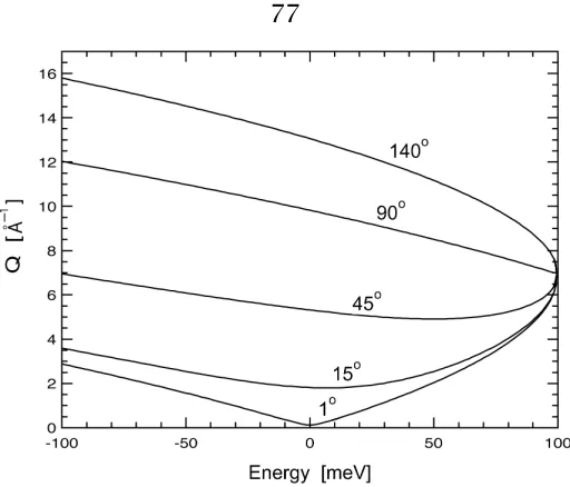
4.6 Kinematic limit . . . 77

4.7 Schematic of the ARCS . . . 79

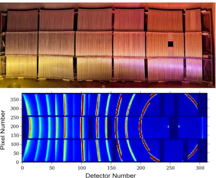
4.8 Detector banks at ARCS and the signal . . . 81

4.9 Multiphonon and multiple scattering fit . . . 84

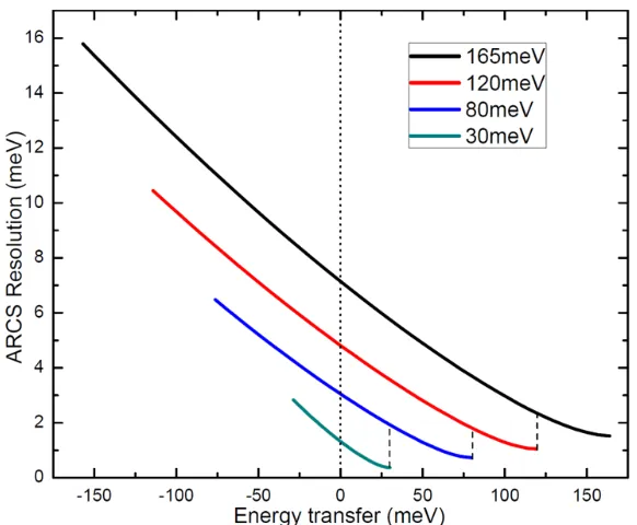
4.10 Resolution functions for ARCS . . . 85

4.11 Schematic of a triple-axis spectrometer . . . 87

4.12 Schematic of HB-3 triple-axis spectrometer at HFIR . . . 89

4.13 Resolution ellipsoids . . . 91

4.14 MICAS furnace . . . 94

4.15 Sample can and its insert . . . 95

5.1 Principles of Raman scattering . . . 99

5.2 Scattered radiation of a polarized incident light . . . 101

5.3 Scattered radiation of an unpolarized incident light . . . 103

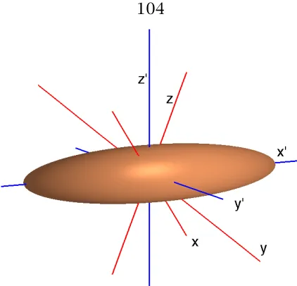
5.4 Coordinate systems for a polarizability ellipsoid . . . 104

5.6 Schematic of a Raman system using 90◦_{geometry . . . 112}

5.7 Schematic of the energy levels for Nd ions in a Nd:YAG laser . . . 114

5.8 Schematic of a Raman system using 180◦_{geometry . . . 119}

5.9 Raman furnace . . . 122

5.10 Schematic of the time-resolved Raman system . . . 125

6.1 Crystal structure of monoclinic hafnia . . . 131

6.2 Raman spectra and phonon DOS of hafnia . . . 133

6.3 Temperature-dependent Raman mode softening in hafnia . . . 135

6.4 Temperature-dependent peak broadening in hafnia . . . 136

6.5 Representative Raman-active normal modes in hafnia or zirconia . . 141

6.6 Broadening vs. softening of Raman modes in hafnia . . . 144

7.1 Comparison of the Raman spectra of hafnia and zirconia . . . 148

7.2 Raman spectra and phonon DOS of zirconia . . . 151

7.3 Temperature-dependent Raman mode softening in zirconia . . . 153

7.4 Temperature-dependent peak broadening in zirconia . . . 154

7.5 Phonon DOS calculated by molecular dynamics for zirconia at differ-ent temperatures . . . 157

7.6 Broadening vs. softening of Raman modes in zirconia . . . 161

8.1 Structure of ScF3 and the mechanical model. . . 168

8.2 Four-energy-overlapedS(Q, E) of ScF3 at 7 K . . . 169

8.3 Neutron-weighted ScF3 phonon DOS and the shifts of phonon peak centers . . . 172

8.4 Calculated phonon dispersions, phonon DOS, and Grüneisen parame-ters of ScF3 . . . 175

8.5 First Brillouin zone of ScF3 and its high-symmetry points . . . 176

8.6 Pair distribution functions from first-principle MD calculations . . . 177

8.8 The angular distribution function for F-Sc-F angle at 300 K from

first-principle MD . . . 178

8.9 First principles MD trajectories and their projections . . . 179

8.10 Phonon modes in ScF3 at R-point (1) . . . 180

8.11 Phonon modes in ScF3 at R-point (2) . . . 181

8.12 Phonon mode R4+ and its frozen phonon potential . . . 182

8.13 Energy levels of the quartic phonon mode R4+ and its frozen phonon potential . . . 186

8.14 Experimental and calculated linear thermal expansion coefficients . 187 8.15 Isosurface of Grüneisen parameter γ = −5 for phonon dispersion branch 4+ . . . 188

8.16 The frozen phonon potential of mode R4+ at Z point . . . 189

9.1 Neutron scatteringS(Q, E) from aluminum at 300 K . . . 197

9.2 Calculated phonon dispersion and linewidth in comparison with neutron spectroscopy measurement . . . 199

9.3 Phonon linewidth distribution over high-symmetry planes. . . 200

9.4 Up-conversion and down-conversion processes for three branches along high-symmetry directions . . . 201

9.5 Distribution of phonon broadenings versus phonon energy at 300 K 202 9.6 Comparison of phonon DOS between calculation and inelastic neutron scattering measurements . . . 204

List of Tables

4.1 Properties of the neutrons . . . 64 4.2 Time-of-flight chopper spectrometers at the SNS . . . 78

5.1 Typical cross sections of common photon proceeses . . . 110

6.1 Raman mode frequencies, fractional atomic contribution for each

mode, and mode Grüneisen parameters of hafnia . . . 137

7.1 Raman mode frequencies, fractional atomic contribution for each

Part I

Chapter 1

1.1

Motivations

Vibrational studies of materials at elevated temperatures are relatively rare. Most phonon work also has emphasized harmonic behavior—non-harmonic effects are often unexplored. However, these non-harmonic effects can be important for many properties of the material, such as thermal transport, phase stability, and thermal expansion.

Harmonic and quasiharmonic models are good approximations for many materials, but anharmonic behaviors are also quite common. Recent work by our group found that adiabatic electron-phonon interactions can have a considerable effect on the vibrational entropy of vanadium metal and A15 vanadium compounds, because of their high electronic density of states near the Fermi level. [1,2] When electron-phonon interactions are not playing major roles, such as in aluminum metal, the phonon-phonon interactions are believed to be the dominant component of the phonon anharmonicity, especially at elevated temperatures. Combined experimental and computational studies on metals and alloys can give insights about the anharmonicity and their effects on phonon dynamics.

Ionic compounds such as oxides or fluorides have dramatic differences from metals and alloys. Firstly, they have much greater variety in structures, many of which have low symmetry. Secondly, most ionic compounds have low electrical conductivity. As a result, electrons are more locally confined, and phonon dynam-ics generally has a larger impact on many properties of these materials. A good understanding of the high-temperature vibrational behavior of these materials can have major benefits for their applications in thermoelectrics, fuel cells, and thermal barrier coating, for example.

1.2

Present Work

inelastic neutron scattering are discussed. Several experiments on phonon an-harmonicity were performed with these experimental methods, and interpreted with computational methods. Aside from the phonon frequency shift, which is typically used to understand vibrational thermodynamics, high-resolution mea-surements of phonon energy broadening allows for an assessment of the origin of the anharmonic behavior.

In Raman spectroscopy studies on the phonon dynamics of hafnia and zirconia, Raman line positions, and shapes of temperatures to 1000 K were measured, and the temperature-dependent Raman peak shifts and broadenings were reported and compared with each other. The modes that exhibit the most anharmonicity were characterized and correlated to the vibrational displacements of individual atoms in the unit cell using both a shell model and density functional theory. It was found that anharmonicity in these systems is rich in information and strongly mode dependent. The discrepancy between the temperature and pressure Grüneisen parameters is surprisingly large. Previous studies have largely neglected these effects and further exploration will definitely advance the understanding of phonons and vibrational entropy.

Cubic scandium fluoride (ScF3) has an enormous negative thermal expansion

over a wide range of temperature. Using time-of-flight inelastic neutron scattering, we found purely quartic transverse modes with an anomalous mode stiffening with temperature, and related these modes to the negative thermal expansion of the DO9 structure using phonon and frozen phonon calculations with first-principles

methods. The vibrational entropy contribution from these soft phonon modes may help to stabilize the cubic phase over a wide range of temperature.

calculations and prior measurements of phonon linewidths at 300 K, and new measurements of the phonon density of states from 7 to 750 K, indicates that the third-order phonon-phonon interactions calculated from DFT can account for the lifetime broadenings of phonons in aluminum to at least 80% of its melting temperature.

Part II

Chapter 2

2.1

Introduction

In physical science, a phonon is acollectiveexcitation of atoms or molecules in condensed matter phases such as solids and liquids. The name “phonon” comes from the Greek word “ϕωνη´”, which translates as “sound” or “voice” because sound is just long-wavelength accoustic phonons. First introduced in 1932 by Russian physicist Igor Tamm, a phonon is referred to as a “quasiparticle”, which represents an excited state in the quantization of the modes of vibrations of elastic structures of interacting particles. [3,4]

Phonons play major roles in solid state physics. They often determine the thermal and electrical conductivities of materials, and sometime have a large impact on a material’s crystal structure as well. A phonon is a quantum mechanical description of a special type of vibrational motion, in which a lattice uniformly oscillates at the same frequency. In classical mechanics this is commonly known as a normal mode, but in quantum mechanical treatments phonons are considered nearly-free particles.

This work will mostly be focused on the dynamics of nuclei in crystals because for phonon dynamics, most of the moving mass is in the nuclei. Theoretical and computational principles of phonons have been elaborated extensively elsewhere. [4–9] This chapter will only briefly restate the basic questions regarding the theory of phonon lattice dynamics, and the following chapter will discuss in more detail the techniques for phonon-related calculations.

2.2

Crystal Lattice

The formalism for phonons is usually developed for solids with long-range peri-odicity: crystal lattices. A perfect crystal lattice can be generated by the infinite repetition in 3-dimensional space of a unit cell defined by three noncoplanar vectors: a1,a2, anda3, which are called the primitive lattice vectors of the

equilibrium position of the origin of the unit celllis

rl=l1a1+l2a2+l3a3. (2.1)

The number of possible arrangements of the lattice vectors are limited, and they are called Bravais lattices. There are 5 Bravais lattices in 2 dimensions (Fig. 2.1) and 14 Bravais lattices in 3 dimensions. A Braivais lattice looks exactly the same from any of the lattice pointsrl.

Figure 2.1: The five two-dimensional Bravais lattices: oblique, rectangular, rhom-bic, hexagonal, and square [12]

Each of the R atoms in one unit cell is assigned an indexκ = 1,2...R. The equilibrium positions of the atoms with respect to the origin of a unit cell are defined as the site vectorsrκ, κ=1,2...R, and the equilibrium position of atom κ in celllis a combination of the two vectors

At finite temperatures the atoms vibrate around their equilibrium positions, adding another time-dependent vector to the instantaneous position of the atoms. Sometimes it is convenient to study Bravais lattices by their reciprocal lattices, which are the Fourier transform of the spatial function of the original lattice, now in

k-space (momentum space). Detailed mathematical and physical descriptions can be found in any solid state physics textbook. [9,10,13] Because of the periodicity of the reciprocal lattice, it is sufficient to study only one primitive cell (Brillouin zone) of reciprocal space. Defined similar to the Wigner-Seitz cell in real space, the volume included by surfaces at the same distance from one site of the reciprocal lattice and its neighbors is the first Brillouin zone. Higher-order Brillouin zones with the same volumes could also be defined. Using the symmetry in the point group of the lattice, the first Brillouin zone can be further reduced to the irreducible Brillouin zone, which is commonly used in computations to reduce to the amount of work.

2.3

Normal Modes

Before discussing normal modes in periodic lattices, first we have a look at vibrations in systems of just a few particles (for example, a CO2molecule). Suppose

the system is made of npoint-mass-like particles interconnected by harmonic springs. There will be 3n equations of motions and 3n degrees of freedom, including 3 translational and 3n−3 vibrational degrees of freedom. The system is completely solvable, albeit extremely difficult to tackle directly when the number of particles becomes large.

the general motions of the system are a superpositions of these normal modes. The modes are "normal" in the sense that they are uncoupled. That is to say, in a perfectly harmonic system, an excitation of one mode will never cause motion of a different mode, i.e, there is no energy transfer between these (harmonic) normal modes.

The same idea applies to solids with periodic lattices as detailed in Section 2.6.3. The evenly spaced energy levels of these harmonic normal modes are exactly how phonons are defined. Solids with more than one type of atom in the unit cell have two types of phonons: acoustic phonons and optical phonons. Acoustic phonons are long-wavelength, coherent movements of atoms out of their equilibrium positions and are named after their close relation to sound waves. They can be both longitudinal (LA, in the direction of propagation) or transverse (TA, perpendicular to the propagation direction). Acoustic phonons mostly have a linear dispersion relationship between frequency and phonon wavevector, in which the frequency goes to zero in the limit of long wavelength. On the contrary, optical phonons are short-wavelength, out-of-phase movements of the atoms in the lattice and only occur if the lattice is made of atoms of different charge or mass. [5] They are named optical because in some ionic crystals, they can be excited by electromagnetic radiation (light) through infrared absorption or Raman scattering. Optical phonons have a nonzero frequency at the Brillouin zone center and because of the symmetry, they show no dispersion near that long-wavelength limit. Similar to acoustic phonons, longitudinal and transverse optical phonons are often abbreviated as LO and TO phonons, respectively.

2.4

Phonon Thermodynamics

notations of Fultz. [16].

Phonons are bosons, so there is no limit to how many phonons can be present in each normal mode. Consider a set ofN coupled modes with the same energyε

and supposemphonons are free to distribute between these modes. Using the entropy equation of Boltzmann, the phonon entropy can be written as:

S =kBlnΩ, (2.3)

whereΩis the number of ways to place themphonons in theNmodes. Notice that the phonons are indistinguishable. Using the binomial result of the combinatorial rule,Ω can be written as:

Ω= (N−1+m)!

(N −1)! m! . (2.4)

In macroscopic systems where the numbers of modesN are large, N−1 can be replaced byN:

Ω= (N+m)!

N! m! . (2.5)

Substituting (2.5) into (2.3), and expanding the factorial using the Stirling approximation of lnx! 'xlnx−x:

S =kBh(N+m)ln(N+m)−NlnN−mlnmi. (2.6)

Assuming the occupancy of each mode isn≡m/N, the entropy per mode can be written as:

S N =kB

h

As a comparison, the entropy per site for fermions is

Sfermi

N = −kB

h

(1−c)ln(1−c)+clnci, (2.8)

wherecis the occupancy of each site. This happens to be the same as the entropy of mixing (wherec is the site occupancy) due to the nature of the Pauli exclusion principle.

With the vibrational entropy per mode (Eq. 2.7), the Helmholtz free energy per mode for a system of oscillators is

F N =

E N −T

S

N =n ε−T kB

h

(1+n)ln(1+n)−nlnni, (2.9)

whereE=n ε is the total phonon energy in the mode.

The equilibrium phonon occupancy nat temperatureT can be calculated by minimizing the free energyF with respect to n. The result:

n(T )= 1 ek_BεT ₋₁

, (2.10)

is the Planck distribution for phonons, or the Bose-Einstein distribution. It is common practice to simplify the expression usingβ=(kBT )−1_.

In a crystalline system, there are a variety of phonon modes with different energies. Using the results above, the phonon entropy of the system can be calculated with the partition function.

For a harmonic crystal, the total vibrational energy capacity is calculated as contributions from a system of independent oscillators. The partition function for a single quantum harmonic oscillator (mode)iat energy i=~ωi, whereωi is the vibrational frequency, is:

Z_i=

∞

X

n

e−β(n+1/2)i ₌ e −βi/2

1−e−βi. (2.11)

total partition function is the product of these single oscillator partition functions,

Z_N =

3N

Y

i

e−βi/2

1−e−βi. (2.12)

Using the thermodynamics relation of the partition function, the phonon free energy and entropy can be calculated as:

Fph= 1 2

3N

X

i

i +kBT

3N

X

i

ln1−e−βi_{, (2.13)}

Sph=kB 3N

X

i

−ln1−e−βi₊ βi

eβi−1

. (2.14)

It is often useful to work with a phonon density of states (DOS), g(), where 3Ng()dphonon modes are in an energy interval d. Note that the phonon DOS

g()here is assumed to be normalized to unity. For a discrete phonon DOS in m

intervals of bin width∆each, the partition function can be computed numerically as:

Z_N= m

Y

j=1

e−βj/2

1−e−βj

!3Ng(j)∆

. (2.15)

It is interesting that the only material parameter relevant to the thermodynamic partition function is the phonon DOS,g().

Using a measured or calculated phonon DOS, the phonon entropy of a harmonic crystal at temperatureT can be written as

Sph=3kB ∞

Z

0

g() h n()+1

ln n()+1

−n()ln n()i

d, (2.16)

phases,αand βbecomes independent of temperature and can be written as

∆S_phβ−α =3kB ∞

Z

0

(gα()−gβ())ln() d. (2.17)

It has been known for a while that phonon entropy is important for crystal stability [17,18] but obtaining an accurate phonon DOS to calculate differences in vibration entropy like ∆Sphβ−α turns out to be difficult and became possible

only recently. [19,20] More details will be discussed in later chapters on these computational and experimental techniques. Although the temperature effects on phonon thermodynamics are also important and will be discussed in subsequent sections, the phonon spectra of solids are mostly determined by phases and compositions. The dominant factors for phonon entropy are the atomic masses

M, and the spring constantskfrom the interatomic force constants, as in a classic harmonic oscillator:

ω=

s

k

M, (2.18)

whereωis the vibrational frequency. For atoms of similar size, it is found that in a solid solution of atoms A and B, with their atomic massesMAandMB, respectively, the phonon entropy upon alloying tends to scale with ln(MA/MB), [16,21] although there is a large scatter in this correlation especially for some of the alloys. This is possibly a consequence of the difference in atom sizes, which cause local stress and as a result, drastically alter the interatomic force constants.

constants.

2.5

Temperature Effects

2.5.1

Harmonic Phonons

In the simplest approximation, where all the oscillators in a solid are harmonic and have fixed frequencies (Einstein model [7]), the heat capacity could be derived from Planck distribution (Eq. 2.10). The heat capacity at constant volumeCV ,i for the modei is

CV,i(T )=kB

_ε

i

kBT

2 _exp(ε

i/kBT )

(exp(εi/kBT )−1)2

, (2.19)

where the temperature derivative of the occupancy distribution is weighted by the energy of the phonon mode. In the high-temperature limit, the result becomes the classic one: one kB per mode.

A Debye model, [7] which treats the vibrations as phonons in a box, assumes a phonon DOS that is a quadratic function of energy, and increases monotonically up to a cutoff energy. (The actual DOS often has a more abrupt rise at low energies that comes from the lower sound velocity of the low transverse modes and a complex structure at higher energies.) The Debye model does predict some general features of the heat capacity a little better, especially in the low-temperature limit. A useful result from this model is the Debye temperature

θD= hνm

k , (2.20)

whereνmis the vibrational frequency at the cutoff energy. Above this temperature, the vibrations in the solid are approaching the classical limit and quantum effects become less important. For pure elements,θD varies from less than 100 K (soft metals) to over 2000 K (carbon).

account for even some of the most basic behaviors of solids. Typically, materials expand when heated, their elastic constants change with temperature and pressure, their specific heats at constant volume or pressure are not equal, and their thermal conductivity is not infinite. We have to go beyond the harmonic approximation to understand these properties. [5,20,23]

2.5.2

Quasiharmonic Thermodynamics

Experimentally, the heat capacity at constant pressureCp is most useful because it can be measured directly by calorimetry:

Cp(T )=T dS

dT

_p. (2.21)

The difference betweenCp andCV is a classical thermodynamic relationship [10]

Cp−CV =9Bvα2_{T , (2.22)}

whereB is bulk modulus,αis the linear coefficient of thermal expansion, andv

is specific volume.

Eq. 2.22can be derived by assuming that the free energy of a crystal comes only from phonons and thermal expansion. The total free energy can be written as

F (T )=Eelas(T )+Eph(T )−T Sph. (2.23)

Phonon energies fall significantly, but thermal occupancy compensates, leading to small net changes inEph.

The elastic energy of thermal expansion is

Eelas= 1 2B

(δV )2 V0 =

9 2BV0α

and the phonon energy and entropy in the classical limit are

Eph(T ) = 3NkBT , (2.25)

Sph(T ) = kB 3N

X

j

ln kBT

~ωj

!

. (2.26)

Assume a linear phonon frequency shift with respect to the change of volume:

ωj =ω0j(1−3αT γ), (2.27)

ln(ωj)'ln(ω0j)−3αT γ, (2.28)

whereγ is the Grüneisen parameter. The phonon entropy can be written as

Sph(T ) =



kB

3N

X

j

ln kBT

~ω0j

!

+9NγαkBT (2.29)

= S_ph0 +Sq, (2.30)

where the first term,Sph0 , is the harmonic phonon entropy atT =0, and the second

term,Sq, is the quasiharmonic part:

Sq =9BV0α2T . (2.31)

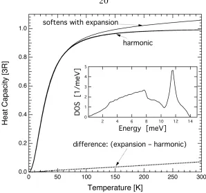
Typical quasiharmonic effects on the heat capacity are shown in Fig. 2.2. Using these results, the total free energy in a quasiharmonic crystal is

F (T )= 9 2BV0α

2_T2_{+3NkBT−T S}0

ph(T )−9NαγkBT

2_{. (2.32)}

The equilibrium thermal expansion coefficient,α, can be calculated by minimizing the free energy with respect toα, giving

α = CVγ

3BV0. (2.33)

Figure 2.2: Heat capacity versus temperature for a simple harmonic model with a phonon DOS unchanged with temperature, and a typical case where the solid expands against its bulk modulus. Inset is the phonon DOS at 0 K. From [16]

comparing the vibrational thermodynamics of different materials at elevated temperatures because it often gives a good accounting of the phonons and thermal expansion, but many exceptions are known. This quasiharmonic approximation assumes that the oscillations in the system are harmonic-like and they change only modestly and predictably with changes in temperature and pressure. Also the phonon lifetimes are long enough so that their frequencies are well defined.

2.5.3

Anharmonic Thermodynamics

It is possible to experimentally determine if a solid is “quasiharmonic” or “anharmonic”. The thermal softening of the phonon modes can give a

mode-averaged Grüneisen parameterγ. The phonon DOS can be used to calculateCV, and conventional measurements can provide B, V0, and α, accounting for all unknowns in Eq. 2.30. If the γ from Eq. 2.30matches the γ from phonon shifts, the solid is “quasiharmonic”.

When phonon softening or stiffening is inconsistent with the Grüneisen param-eterγ needed for equality in Eq. 2.30, the solid is anharmonic. The anharmonicity may be a result of electron-phonon interactions, changes in electronic structure with temperature, or higher-order phonon-phonon interactions. It is generally diffi-cult to determine the sources of non-harmonic behavior and their contributions to the entropy. [7] Usually the effects of electron-phonon interactions are important only at low temperatures and are often ignored as a source of anharmonicity when the temperature is higher. Substantial deviations from quasiharmonic behavior are known for many metal [16] and non-metal systems.

2.5.4

Phonon Entropy

The logarithm definition of the entropy makes it easy to split the total entropy into uncorrelated subsystems

S=kBlnΩ=kBln



 Y

i

Ωi



=kB

X

i

lnΩi=

X

i

Si, (2.34)

where i denotes the index of subsystems. It may be necessary to correct for the interactions between these subsystems (cross terms) but they are usually small enough to be treated as perturbations. The total entropy of a crystal then can be written as the sum of configurational, phonon, electron, electron-phonon interaction, magnetic, and nuclear contributions

We will ignore other effects, such as electronic, magnetic, and nuclear ones, and only consider phonon harmonic, quasiharmonic, and anharmonic contributions

Sph=S_ph0 + +Sq+Sanh (2.36)

for now. The temperature dependence of the entropy can be written as:

dS(T , V )

dT = ∂S ∂T _V + ∂S ∂V _T dV

dT. (2.37)

The harmonic part of the vibrational entropy can be calculated with a phonon DOS from low temperature measurement or calculation. The harmonic phonons undergo no change with respect to the temperature or volume, and as a result the temperature dependence of harmonic entropy only occurs because of the change in the Planck occupancy with temperature.

For quasiharmonic phonons, their frequencies depend on volume only and they make a contribution only through the second term on the right-hand side of Eq. 2.37.

∆Sq = ∂S

∂V T dV

dT∆T (2.38)

Using the Grüneisen parameter to describe the frequency change with temperature, the quasiharmonic contribution is

∆Sq =9Bvα2∆T . (2.39)

on the thermal expansion, but it does change the phonon frequencies by 4-phonon process. The second term is associated with changes of the interatomic force constants with volume. Although the quasiharmonic contribution is expected to account for most of this effect, it is only correct to first order [20]. For example, the phonon linewidth broadening from the cubic term in the interatomic potential alters the vibrational entropy. The quasiharmonic contribution accounts for shifting of the phonon frequencies but misses those higher-order terms.

2.5.5

Electronic Entropy

Unlike phonons, which are bosons, electrons fill the states up to the Fermi level, even at absolute zero temperature. The electronic entropy arises from the thermal excitation of electrons around the Fermi level and can be written as:

Sel= −kB ∞

Z

−∞

[(1−f )ln(1−f )+flnf ]n(ε)dε, (2.40)

wheref (ε, T )is the Fermi distribution function andn(ε) is the electronic density of states. Similar to the phonon entropy, the total electronic entropy can be split into contributions from the ground state and the thermal expansion (lattice dilation):

Sel=SelG+SelD. (2.41)

2.6

Lattice Dynamics

2.6.1

Interatomic Force-Constants

For atom vibrations in crystals, only the motions of the nucleus are relevant because the mass of the electron is negligible in comparison. Ignoring the detailed mechanism of these interactions [8,20], the Hamiltonian for nuclear motions can be written as [24,25]

Hn=X l,κ

p2_lκ 2mκ

+Φ, (2.42)

where Φis the potential energy, pis the momentum vector, andlandκ are the labels of atom and unit cell, respectively. The instantaneous positionRlκ(t) of atomlκ at timet is

Rlκ(t)=rl+rκ +ulκ(t), (2.43)

where the atomκ in the unit celllvibrates about its equilibrium with the displace-mentulκ(t).

We expand the total potential energy Φin a Taylor series about these equilib-rium positions

Φ = Φ0+

X

αlκ

Φαlκuαlκ

+1 2

X

αlκ

X

α0_l0_κ0

Φ_αα0_lκl0_κ0u_αlκu_α0_l0_κ0+..., (2.44)

whereα= {x, y, z}are the Cartesian components, the coefficients of the Taylor series are the derivatives of the potential with respect to the displacements

Φαlκ =

∂Φ ∂uαlκ 0 , (2.45)

Φ_αα0_lκl0_κ0 = ∂

2_Φ

∂uαlκ∂uα0_l0_κ0

andΦ0is the static potential energy of the crystal. Because the force on any atom

must vanish in the equilibrium configuration,

Φαlκ =0. (2.47)

As an approximation that we will revisit in the next section, we neglect terms of order three and higher in the displacements in Eq. 2.44. The Hamiltonian can be written as

Hn =X lκ

p2_lκ 2mκ

+Φ0+

1 2

X

αlκ

X

α0_l0_κ0

Φαα0_lκl0_κ0u_αlκu_α0_l0_κ0. (2.48)

This is the harmonic approximation of lattice dynamics. It is possbile to rewrite the Hamiltonian in matrix form

Hn=X lκ

p2_lκ 2mκ

+Φ0+

1 2

X

lκ

X

l0_κ0

uT_lκ Φlκl0_κ0 u_l0_κ0, (2.49)

where Φlκl0_κ0 is a 3×3 force-constant matrix defined for each atom pairlκ and

l0_κ0 _{((l, κ)}

≠(l0, κ0)):

Φlκl0_κ0 =[Φ_αα0_lκl0_κ0] . (2.50)

This is the famous Born-von Kármán model. [8,26] If(l, κ)=(l0_{, κ}0_),Φ

αα0_lκlκ is a “self-force constant”, determined by the requirement of no overall translation of

the crystal

Φ_lκlκ = − X

(l0_,κ0₎ ≠(l,κ)

Φ_lκl0_κ0. (2.51)

Φlκl0_κ0 must be real and symetric.

Φlκl0_κ0 =



    

a b c

b d e

c e f



    

(2.52)

To satisfy the translational symmetry, the force constant matrices must also have the following property

Φ_lκl0_κ0=Φ_0κ(l0_−l)κ0 =Φ_(l−l0_)κ0κ0. (2.53)

It should be noted that the interatomic force constants, such asΦαα0_lκl0_κ0, are in fact not constant but functions of temperature and lattice parameters.

2.6.2

Equations of Motion

Using the the harmonic approximation and the potential above, the equations of motion for nuclei are

mκulκ(t)= −

X

l0_,κ0

Φlκl0_κ0u_l0_κ0(t). (2.54)

There are 3× R ×Ncell _{equations of motion for a finite crystal containingN}cell

unit cells, each containingRatoms. [8]

It is easily calculated that for any crystal of reasonable size (on the order of 1023 _{atoms) the atoms on the surface account for only a very small fraction of}

plane waves of wavevectork, angular frequencyωkj, and “polarization”eκj(k)

u_lκkj(t) =

s

2_~

N mκωkj

e_κj(k)ei(k·rl−ωkjt)_{, (2.55)}

= _~

v u

t2n(εkj, T )+1

N mκεkj

eκj(k)ei(k·rl−ωkjt), (2.56)

where we take the real part to obtain physical displacements. The phase factor, eik·rl_{, provides all the long-range spatial modulation, while the dependence onκ,}

a short-range basis vector index, is placed in the complex constante_κj(k). It is convenient for this constant and the exponential to have modulus unity. j is the “branch index” discussed below and there are 3Rdifferent such branches from

symmetry.

2.6.3

The Eigenvalue Problem of the Phonon Modes

The polarization vectors,eκj(k), contain all information on the excursion of each atom κ in the unit cell for the phonon mode k, j, including the displacement direction of the atom and its relative phase with respect to the other atoms. These “polarization” vectors and their associated angular frequenciesωkj(normal modes) can be calculated by diagonalizing the “dynamical matrix” D(k). The detailed descriptions can be found elsewhere. [8,23–25]

The dynamical matrix can be obtained by substituting Eq. 2.56into2.54. It has the dimensions 3N×3N and is constructed from 3×3 submatrices Dκκ0(k)

D(k)=

     

D11(k) . . . D1N(k) ..

. . .. ...

DN1(k) · · · DNN(k)

      , (2.57)

matrixΦlκl0_κ0

Dκκ0(k)= 1 √

mκmκ0

X

l0

Φ0κl0_κ0eik·(rl0−r0). (2.58)

To simplify, the equations of motions (Eq. 2.54) with the plane wave solutions (Eq. 2.56) can be represented as an eigenvalue problem:

D(k)ej(k)=ω2kjej(k), (2.59)

where

ej(k)=

               

ex1j(k)

ey1j(k)

ez1j(k)

ex2j(k) .. .

ezNj(k)

                (2.60)

is the eigenvector(s).

It can be shown that the dynamical matrix D(k)is hermitian for any value of k. As a result it is thus fully diagonalizable and the eigenvaluesω2_kj are real. The eigenvectors and eigenvalues of the dynamical matrix evaluated at a particular wavevector k correspond to the 3R eigenmodes of vibration of the crystal for that wavevector. It should be noted that the angular frequency (ωkj) dependence on the wavevector (k), called a dispersion relation, can be quite complicated. The speed of propagation of phonons in solids (speed of sound) is given by the group velocity as the slope of this relation

vsound =vg= ∂ωkj

instead of the phase velocity

vp= ωkj

k . (2.62)

2.6.4

The Phonon Density of States

With the phonon vibrations calculated above, it is straightforward to calculate the phonon density of states (DOS) of a crystal. This is done by diagonalizing the dynamic matrixD(k)at a large number ofkpoints in the first Brillouin zone, and then binning them into the DOS histogram.

Similarly, a phonon partial DOSgd(ε), which gives the spectral distribution of motions by one atom speciesdin the unit cell, can be obtained through weighting the vibrational contribution

gd(ε)=

X

k|

X

ακj

δdκ|eακj(k)|2g(ε). (2.63)

Because the eigenvalues of the dynamical matrix are normalized for eachkas

X

ακj

|eακj(k)|2=1, (2.64)

the total DOS is the sum of the partial DOSs of all atoms in the unit cell,

g(ε)=X d

gd(ε). (2.65)

2.6.5

Group Theory

With group theory, it is possible to find eigenvectors and eigenvalues without diagonalizing the dynamical matrix. [8] Maradudin and Vosko’s review showed how group theory can be used to understand the normal modes of crystal vi-brations and classify them. [27] In their work, the degeneracies of the different normal modes were addressed rigorously, and their association with the symmetry elements of the crystal were used to label them. In the same issue of the journal, Warren discussed the point group of the bond, [28] which refers to the real space symmetries of the interatomic interactions, i.e., how the force constants transform under the point group operations at a central atom.

2.7

Phonon-Phonon Interactions

Due to the huge mass ratio (1 : 105_{), it is often reasonable to assume that the}

nuclear motions are slow enough so that the electron levels adapt continuously to the evolving structure (Born–Oppenheimer approximation or adiabatic approxi-mation). [4,8,10] This assumes that the electronic and nuclear systems are well separated and any interactions can be accounted for as perturbations. The full Hamiltonian of the crystal can be written as

H =Hn+He+Hep, (2.66)

where He and Hep are the contributions from the electron, including electron-electron interactions and thermal electron-electronic excitations, and from electron-electron-phonon interactions (EPI), respectively.

in the Taylor series of Eq. 2.44:

Hn =Φ0 +

X

κ p2

κ 2m +

1 2!

X

κα

X

κ0_α0

Φαα0_κκ0u_ακu_α0_κ0

+ 1 3!

X

κα

X

κ0_α0

X

κ00_α00

Φ_αα0_α00_κκ0_κ00u_ακu_α0_κ0u_α00_κ00

+ 1 4!

X

κα

X

κ0_α0

X

κ00_α00

X

κ000_α000

Φαα0_α00_α000_κκ0_κ00_κ000u_ακu_α0_κ0u_α00_κ00u_α000_κ000+...,(2.67)

where we assume one atom per unit cell.

The transformation to normal coordinates for an infinite periodic crystal is

Uki =

1 √

N m

X

rκ

urκe−iki·rκ, (2.68)

and by Fourier inversion

ur~κ =

1 √

N m

X

ki

Ukie

+iki·rκ_{. (2.69)}

Substituting this into Eq. 2.67, we identify the Fourier transform ofΦαα0_κκ0, and use it to define the dynamical matrix.

It is usually easier to work with the quantized phonon field using the second quantization formalism. The phonon field operator is

Aki =aki+a † −ki =A

†

−ki. (2.70)

Constructed from the momentum and position operators of the Hamiltonian, the raising and lowering operatorsa†_ki and aki create and annihilate the phonon

ki, respectively, similar to raising and lowering operators for a simple quantum harmonic oscillator. [29]

This is the occupation number representation, wherenphonons of wavevec-tor ki are created with n raising operations as

displacement operators in this representation are

u(rκ)=

X

ki

s

~

2N m ωki

e(ki)eiki·rκAki. (2.71)

By substituting this into Eq. 2.67, we have

ˆ

Hn = Φ0+

X

ki

~ωki

a†kiaki+

1 2 + X ki X kj X kk

V (k_i,k_j,k_k) AkiAkjAkk

+ X ki X kj X kk X kl

V (ki,kj,kk,kl) AkiAkjAkkAkl+..., (2.72)

where the first sum on the right-hand side includes both the kinetic energy and the harmonic part of the potential energy, and theV are related to the Fourier transforms ofΦ. For example, the cubic term is

V (ki,kj,kk) = 1 3! v u u t 1

N m3

~

2

3 ₁

ωkiωkjωkk

δ(ki+kj+kk−g)

× X ~ rκ

e(k_i)e(k_j)e(k_k)e+i(ki+kj+kk)·rκ_Φ

α,α0_,α00_κ,κ0_,κ00, (2.73)

where the factorδsignifies that the conservation of lattice momentumki+kj+kk = g, whereg is a reciprocal lattice vector. [9] The cubic (V (ki,kj,kk)) and quartic (V (ki,kj,kk,kl)) terms give the energies of “phonon-phonon interactions” because they alter the phonon energies when larger vibrational displacements are present in the crystal.

Although not obvious at first sight, details of the phonon dispersions are crucial for an attempt to calculate anharmonic behavior because of the conservation of energy and momentum. For example, for three phonon process,k+k0_=k00_+g

andε+ε0_=ε00 _{must be satisfied simultaneously. Most phonon dispersions are}

For larger phonon wavevectorsk, momentum conservation is possible by adding a reciprocal lattice vectorg, and the idea is that the momentum transferred to the entire crystal occurs with zero energy because of the large mass of the crystal. Such “umklapp” processes allow many more three-phonon interactions, but the phonon wavevectors must be of length comparable to the reciprocal lattice vector for this to be possible.

It is important to determine how many terms are needed in Eq. 2.72to account accurately for anharmonic behavior. The higher-order terms become progressively smaller, but the requirement of energy and momentum conservation restricts the allowable three-phonon processes, so fourth-order anharmonicity can be as significant as the third. Also, four-phonon processes can be generated from two three-phonon processes.

For systems where the electron-phonon interaction (EPI) has little role, such as ionic isolators, the anharmonic phonon effects are solely from phonon-phonon interactions. These cause the energies of phonons to be shifted and broadened. Treating all the components as perturbations, the energy shifts can be written as

∆ω(q)=∆ωq(q)+∆ω3(q)+∆ω4(q), (2.74)

where the terms on the right-hand side are quasiharmonic, third-, and fourth-order contributions, respectively. On the other hand, the energy broadening is believed to be usually dominated by the third-order contribution. The related theory has been discussed in detail. [4,15,23,30–33]

2.8

Electron-Phonon Interactions

energy of deformation is electronic in origin, it transfers to kinetic energy in the motion of the nuclei. In a perfectly harmonic system, the electron-phonon interaction affects equally the energies of the electrons and the phonons. If the electrons were always in their ground states, all this energy of deformation would be associated with phonons only. Treating the electron system and the phonon system as two independent thermodynamic systems becomes inconsistent at finite temperature, however, because the presence of phonons alters the thermal excitations of electrons. [4]

Classically, the electron-phonon interaction (EPI) requires the coordinates of the electrons{rel_λ}, and the coordinates of the nuclei{rn_j}[22]

Hep=X λ,j

v(rel_λ,rn_j). (2.75)

The EPI in the “adiabatic approximation” does not allow the nuclear kinetic energy to alter the electron states. The “non-adiabatic” electron-phonon interaction accounts for how the electronic states are altered by the nuclear kinetic energy, not the potential energy of displaced nuclei, as for the adiabatic case. The non-adiabatic EPI requires no thermal activation, and can be responsible for superconductivity.

In the adiabatic picture, unique electron eigenstates exist for a snapshot of the nuclear thermal displacements, which evolve continuously as the nuclei move. For a given electronic structure, the adiabatic electron-phonon interaction is proportional to the number of phonons,n(ε, T )+1/2, times the difference of electron occupancy with respect to the ground state,f (T )−f (0), wheref (T ) is the Fermi-Dirac distribution. When there are sharp features in the electronic DOS near the Fermi level, there will be other temperature dependences associated with the thermal sampling of the excited electron states.

of long wavelength,

HD ep= −

X

λ

D∆(rel_λ) (2.76)

where ∆(rel_λ)is the fractional change in volume at rel_λ, and D is a “deformation potential”, typically a few eV. This simple approach is convenient because∆(rel_λ)

is related to the displacementuas through its divergence: ∆(rel_λ)= ∇ ·u, so

HD

ep= −D

X

λ

∇ ·u(rel_λ). (2.77)

For longitudinal phonons

~ e(ki)=

ki

ki

, (2.78)

and Eq. 2.76can be written as

ˆ

HD

ep= −iD

X

rel_λ

X

ki

s

~

2N m ωki

|ki|eiki·r el

λ A_k

i. (2.79)

Similar to the second quantization of phonons, fermion field operators for the electron are

Ψ†(rel_λ)=X

kλ

C_k†_λe−ikλ·relλ, (2.80)

which when applied to a multi-electron state, places an electron in the state k_λ. When small, ˆHD

ep is a perturbation that mixes electronic states and can be

evaluated by using the fermion field operatorsC and C†_{, where the exponential}

the annihilation operators

ˆ

HepD = −iD

s

~

2N m

electron X kλ phonon X ki s ki cL

AkiC †

kλ+kiCkλ, (2.81)

plus an analogous term with A†kiCkλ+kiC †

kλ for phonon creation. Here we used

a linear dispersion relationship ωL = cLki for long-wavelength, longitudinal acoustic phonons.

In general, there are two lower-order terms that are used to describe the electron-phonon interaction. The first is a generalization of the previous result for the deformation potential with long-wavelength, longitudinal acoustic phonons

ˆ

Hep1 =

X

ki

X

kλ

Vep(ki,kλ) AkiC †

kλ+kiCkλ, (2.82)

which accounts for the processes where an electron is excited from state kλ to kλ+ ki, simultaneously with the annihilation of a phonon in state ki, or creation of a phonon in state −ki. The second low-order term for electron-phonon coupling ( ˆH2

ep) includes a factor from second-order perturbation theory,

P

k0hk|Ω|k0ihk0|Ω|ki. There is no change of electron state by this process,

never-theless, the scattering into the virtual states alters the self-energy of the electron. Calculating the thermodynamic effects of electron-phonon coupling requires averaging over all electron states near the Fermi surface separated by kj and differing in energy by a selected_~ω. Most work on electron-phonon coupling has focused on superconductivity, where_~ωis rather small, and the electron states are close enough to the Fermi surface that it is reasonable to use ground-state Fermi surface properties. The Éliashberg coupling functionα2_{g(ω), whereg(ω)}

is the phonon DOS, accounts for all scattering between electron states on the Fermi surface. The “electron-phonon coupling parameter”λis calculated by weighting byω−1

2

Zωmax

0

α2_g(ω)

Chapter 3

3.1

Introduction

While the advances in computational tools and techniques made possible many, things believed impractical only a couple of decades ago, one still has to make many approximations when doing most computational work. For computational solid state physics, it is the task of theoretical studies to decide on the best approximations to reduce the computational difficulties while preserving as much information as possible about the objects of study. Improvements in the power of computers rarely make sudden breakthroughs, so simulations often need breakthroughs in theory.

Computational science on atomic and subatomic scales benefits all disciplines of science, such as chemistry and bio sciences, but it is especially important for physical sciences. In materials science, we are mostly interested in the simulations on the level of the electronic structure and the levels of crystals or molecules. Predicting the properties of known materials, especially under extreme condi-tions such as high temperatures, high pressure, or high radiation, and designing materials with desired properties under these conditions, are the ultimate goals of computational materials science. We will only briefly review the computational techniques used for phonon studies in this chapter. More detailed discussion can be found in many books. [5,34–38]

As for all computational problems, there is always a compromise between accuracy and speed or time. It is important to select the right tools for the problem at hand, often depending on the size of the systems.

3.2

First-Principle Methods

3.2.1

Many-Body Problem

exact Hamiltonian of such as a system can be written precisely as:

H = −X i

~2

2me∇ 2

i + 1 2

X

i6=j

e2

r_i−r_j

−X I,i

ZIe2 |ri−RI|

−X I

~2

2MI

∇2_I + 1 2

X

I6=J

ZIZJe2

R_I−R_J

,

(3.1) where the terms on the right-hand side correspond to the kinetic energy of elec-trons, potential energy between elecelec-trons, potential energy between electrons and nuclei, kinetic energy of nuclei, and potential energy between nuclei, respectively. All the potential energies are from Coulumbic interactions. The uppercase and lowercase subscripts label the nuclei and electrons, respectively. M is the nuclear mass,me is the electronic mass,Z is the atomic number of nuclei, and Randr donate positions of nuclei and electrons, respectively.

Because electrons have to be considered as quantum particles, the problem comes down to solving the many-body wave functions from the Schrödinger equation. This problem is extremely difficult to tackle directly, even with a system made of only a couple of particles. It is even difficult numerically. The computational cost scales asO(eN_{), where N is the size of the system. For any} other system of practical size, it is necessary to resort to a few approximations.

3.2.2

Hartree-Fock Method

Using the Born-Oppenheimer approximation as discussed in last chapter, it is pos-sible to solve problems at the electronic structure level by isolating the electronic degrees of freedom and placing the nuclei in fixed configurations. In 1928, Hartree suggested an approximation in which the system is reduced to one-electron model where the interactions from other electrons are treated as a mean field. As a result, the total wave function is just the product of the many one-electron wave functions. This is a good starting point, however, it missed some important effects, such as the Pauli exclusion principle and the exchange and correlation energies from the many-body nature of the system.

combinations of non-interacting one-electron wave functions in the form of a Slater determinant

Ψ(r_i)= √1

n!

Ψ1(r1) Ψ2(r1) . . . Ψn(r1)

Ψ1(r2) Ψ2(r2) . . . Ψ_n(r2)

..

. ... . .. ...

Ψ1(rn) Ψ2(rn) · · · Ψn(rn)

, (3.2)

where n is the number of electrons in the system. It solves the problem of antisymmetry, ensuring that the sign of the total wave function will change when two electrons are switched, and no electrons will share a same state.

Under the Hartree-Fock approximation, the total energy can be written as a sum of kinetic, electron-nuclear, Hartree, and exchange energies

E=Ek+Ee−n+EH+Ex, (3.3)

where the Hartree energyEH is determined by the mean-field Hartree treatment and the exchange energyEx corrects for the energy difference as a result of the antisymmetry. Note that we are still missing the correlation energies from the interactions of the spins between electrons, but they can be treated similarly. The computational cost of Hartree-Fock model scales asO(N4_{), whereN is the size}

of the system.

3.2.3

Variational Principle and Self-Consistent Field Method

In practice, the wave functions are usually optimized iteratively using a self-consistent field (SCF) method. A random or a typical wave function is used as the starting point. The electron densities are calculated with these wave functions and then used to obtain the total energy. Using these results, it is possible to solve the equations to have a new set of energies and wave functions for each electron. This process is done iteratively until the changes to wave functions are below a certain threshold.

3.3

Density Functional Theory

3.3.1

Hohenberg-Kohn Theorems

It was not until the 1960s when Hohenberg and Kohn showed by their two theorems that it is possible to solve the problem using only the electronic density ρ(r), that first principles calculations on systems larger than a couple of dozen atoms were made possible. This electron density of states is defined as the sum of all occupied orbitals (i)

ρ(r)=X i

φ_i(r)

2

, (3.4)

which is normalized to the total number of electrons, n,

Z

ρ(r)dr=n. (3.5)

The first HK theorem states that the external (electron-nuclear) potentialVe−n

is uniquely determined by the ground state electron densityρ0(r). BecauseVe−n

determines the Hamiltonian, and thus the ground state and its densityρ0(r), the conclusion is that there is a one-to-one relationship between the ground-state densityρ0(r)and the external potentialVe−n for the electrons. As a consequence, the Hamiltonian and every property of the system is determined fromρ0(r).