Multi Model Inference Ranking and Applications to Physics at the Large Hadron Collider

(1)

and Applications to Physics at the Large Hadron Collider

Thesis by

Val`ere Lambert

In Partial Fulfillment of the Requirements for the Degree of

Bachelors of Science

California Institute of Technology

Pasadena, California

2014

(2)

c 2014

Val`ere Lambert

(3)

Acknowledgements

I would like to express my deepest gratitude to my thesis advisor, Maria Spiropulu, whose faith, determination and enthusiasm not only opened the door for my research in High

En-ergy Physics but also inspired me to continue on in the field.

I would also like to extend my gratitude to Harvey Newman for his inspiration and sup-port, not only for myself but for the entire undergraduate research population.

I want to express my whole-hearted appreciation for my co-mentor, Alex Mott, who has

been my role model throughout this experience. Without his guidance and patience, this thesis would surely not have been possible.

I would also like to thank Adi Bornheim, Cristian Pe˜na, Jan Veverka, Si Xie and the other

members of the Caltech High Energy Physics group for helping, inspiring and shaping me throughout my research over the past few years.

Finally, I thank the wonderful people who raised me, whose love and support were integral

(4)

(5)

Abstract

In the measurement of the Higgs Boson decaying into two photons the parametrization of an appropriate background model is essential for fitting the Higgs signal mass peak over

a continuous background. This diphoton background modeling is crucial in the statistical process of calculating exclusion limits and the significance of observations in comparison

to a background-only hypothesis. It is therefore ideal to obtain knowledge of the physical shape for the background mass distribution as the use of an improper function can lead

to biases in the observed limits. Using an Information-Theoretic (I-T) approach for valid inference we apply Akaike Information Criterion (AIC) as a measure of the separation for a

fitting model from the data. We then implement a multi-model inference ranking method to build a fit-model that closest represents the Standard Model background in 2013 diphoton

data recorded by the Compact Muon Solenoid (CMS) experiment at the Large Hadron Collider (LHC). Potential applications and extensions of this model-selection technique

(6)

(7)

List of Figures

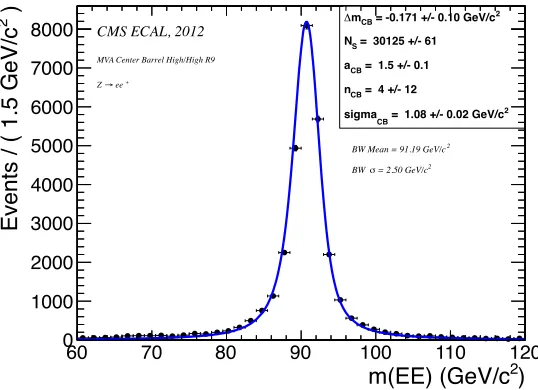
2.1 Comparisons of fits for exponential and power truth models. . . 16

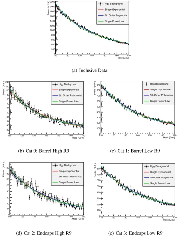
3.1 Fits of various background model families to 2013H →γγdata categories. One sees that there is no ad-hoc method for determining which family of functions is appropriate for modeling the background. . . 21

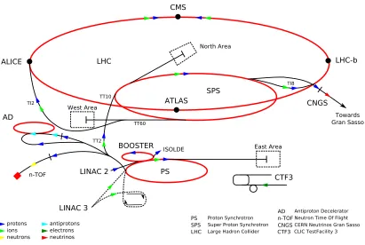
3.2 A schematic diagram of the LHC accelerator complex. Protons are initially accelerated in the LINAC linear accelerator and then injected into the PS

Booster to reach a kinetic energy of 1.4 GeV. They then enter the Proton Synchrotron ring, are accelerated to 25 GeV, and then further accelerated to

450 GeV in the Super Proton Synchrotron (SPS). They are finally accelerated to the maximum energy after being injected into the LHC [31]. . . 24

3.3 A slice diagram depicting the various layers of the CMS detector [31]. . . 25

3.4 Fits of ”composite” background model to 2013H→γγ data categories. . . 29

3.5 Distribution of background events within signal region for composite models derived from 800 toy trials of randomizedH →γγsamples . . . 32

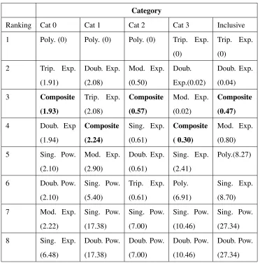
4.1 Fit of invariant mass peak forZ → ee decay for extraction of mass resolu-tion,σCB, and scale,∆mCB [16]. . . 45

4.2 Diagram of CMS electromagnetic calorimeter (ECAL) exhibiting

compart-mentalization of the Barrel and Endcaps [13]. . . 47

4.3 Feynman Diagram for Z boson radiating into two leptons and a photon. . . . 48

4.4 An example of the reconstructedµµγ peak and fit with extracted resolution

(10)

4.5 An example of modeling ofEγ response peak by Gaussian (Top Left). The

data and the fit function are displayed on a logarithmic y-axis scale (Top

Middle). The data corresponds to photons in the ECAL barrel withET >25

andR9 >0.94. . . 50

4.6 Barrel resolution contributions with Data fits on top, Monte Carlo fits in the mid row and Monte Carlo Truth on bottom. . . 57

4.7 End Caps resolution contributions with Data fits on top, Monte Carlo fits in the mid row and Monte Carlo Truth on bottom. . . 58

4.8 Resolution Contributions in bins of pile up and detector location . . . 59

5.1 Photon mistagging efficiences due to gluons faking photons, on the left, and quarks faking photons, on the right. . . 66

5.2 Normalized distributions of ∆Rγγ and min(∆Rγb) are shown for the

di-Higgs signal, thet¯tH background and the QCD non-resonant backgrounds . 68

5.3 Normalized distributions of ∆Rbb after the ”Selection A”requirements are

shown for the di-Higgs signal, the t¯tH background, and the QCD

non-resonant backgrounds. . . 69

5.4 Normalized distributions of thepT of the di-Higgs system (a), the diphoton

system (b), and the di-bjet system (c) are shown for the di-Higgs signal, the t¯tH background, and the QCD non-resonant backgrounds. The distribution

of the sum of thepT of the diphoton system and thepT of the di-bjet system

is shown in (d). . . 69

5.5 The distribution of the diphoton and di-bjet mass for the QCD b¯bγγ back-ground process, after the various event selection schemes. The diphoton

mass distributions are shown on the left and the di-bjet mass distributions are shown on the right. The selections are in descending order of A, B and C. 71

5.6 Optional caption for list of figures . . . 73

5.7 The average expected relative uncertainty on the di-Higgs cross section mea-surements are shown as a function of the assumed widths of the diphoton

(11)

(12)

(13)

List of Tables

2.1 Interpretation of empirical support for AIC distances [11] . . . 14

2.2 Model set used for closure tests. . . 15

2.3 MMI closure results for Single Exponential Truth Model . . . 16

2.4 MMI closure results for Single Power Law Truth Model . . . 17

3.1 Model set of plausible functions for MMI process. . . 28

3.2 AIC results and weights for Standard Model background in 2013H → γγ data. The resulting selected ”best” models for each category are in bold. . . . 30

3.3 Ranking of models for each cut category based on value of−2Log(L)where rank 1 is assigned to the model with the minimized negative log likelihood. The difference between−2Log(L)for each model and the minimized value is shown in parentheses next to the corresponding model. . . 31

3.4 Estimated bias of from the various fit models to the signal region of 123 to 127 GeV for the single exponential truth model. . . 34

3.5 Estimated bias of from the various fit models to the signal region of 123 to 127 GeV for the double exponential truth model. . . 34

3.6 Estimated bias of from the various fit models to the signal region of 123 to 127 GeV for the triple exponential truth model. . . 35

3.7 Estimated bias of from the various fit models to the signal region of 123 to 127 GeV for the modified exponential truth model. . . 35

3.8 Estimated bias of from the various fit models to the signal region of 123 to 127 GeV for the 5th order polynomial truth model. . . 36

(14)

3.10 Estimated bias of from the various fit models to the signal region of 123 to 127 GeV for the double power law truth model. . . 37

3.11 Estimated bias of from the various fit models to the signal region of 123 to 127 GeV for theH →γγtruth model. . . 37

3.12 Estimated slope of various fit models atmH = 125GeV for a single

expo-nential truth model. . . 38

3.13 Estimated slope of various fit models at mH = 125GeV for a double

3.14 Estimated slope of various fit models atmH = 125GeV for a triple

3.15 Estimated slope of various fit models at mH = 125 GeV for a modified

exponential truth model. . . 39

3.16 Estimated slope of various fit models at mH = 125 GeV for a 5th order

polynomial truth model. . . 40

3.17 Estimated slope of various fit models at mH = 125GeV for a single power

law truth model. . . 40

3.18 Estimated slope of various fit models atmH = 125GeV for a double power

law truth model. . . 40

3.19 Estimated slope of various fit models at mH = 125 GeV for the AIC

com-posite model from Inclusive 2013 data. . . 41

4.1 Data and Monte Carlo used in the study ofZ →µµγ events . . . 51 4.2 Expected contributions to the CMS ECAL energy resolution [29]. . . 56

5.1 Expected event yields for 3ab−1 of integrated luminosity for the di-Higgs signal and background under various event selection schemes . . . 70

5.2 Expected event yields for 3ab−1 of integrated luminosity estimated for high pile up scenario expected for the HL-LHC. The event yield reflect ”Selection

B” requirements within three different mass windows. . . 77

5.3 The average expected relative uncertainties on the di-Higgs cross section

(15)

Chapter 1

Introduction

Scientific modeling involves the generation of conceptual or mathematical models to ex-plain relations revealed through experimental data. Traditional methods for model testing

consist of defining a single alternative hypothesis to a null hypothesis. Test statistics are then used to assign probabilistic values for the null hypothesis that define statistical

signifi-cance. However, these methods are inferentially limited and do not include the uncertainty associated with model selection [17]. In terms of the test statistics, if the probability of

the null hypothesis is considered to be low then one concludes that the alternative is a better choice by default. However, the alternative hypothesis may never be tested and the

probabilities of the null and alternative hypotheses are uncertain. In effect, the traditional pair-wise hypothesis testing only provides a measure of how good one hypothesis is in

re-lation the second, yet neither is confirmed to fit the data well [9].

A measure of agreement in a global model is needed in order to determine a more rig-orous method of model testing. The desired system would involve evaluating the relative

worth of alternative hypotheses other than just a one-sided measure of the probability. The conventional methods for model testing can be replaced with Information-Theoretic

meth-ods, which provide a strict measure of evidential strength for both the null and alternative hypotheses [17]. These IT methods determine an approach for producing an a priori set

of hypotheses and means for quantifying the data based on evidence as well as a ranking of each hypothesis. Such methods use tools such as Kullback-Leibler information, which

(16)

wishes to minimize the K-L information and select the model that is closest to representing reality [11].

The primary goal is be to determine a method of avoiding the bias of pair-wise

hypoth-esis testing in order to produce more robust inference results. Given a data set and multiple models corresponding to a phenomenon one wishes to be able to determine a measure of

separation or entropy from which to assign a distance for each model from the data [11]. A ranking for the models can be produced according to this index and then an

appropri-ate weight may be assigned to each model. One would potentially be able to isolappropri-ate data signal forms using the model weights to determine a fundamental expression for that

phe-nomenon [9].

In this study, we develop a multi-model inferencing (MMI) scheme using directional sep-aration as a method for calculating and assigning weights for models in relation to the

data. A substantial portion of the Caltech High Energy Physics group with Compact Muon Solenoid (CMS) Collaboration has been highly involved in the analysis of the Higgs

bo-son decaying into two photons. Due to degraded conditions at the Large Hadron Collider (LHC) from increased pile up, extensive work must be done to select a correct modeling of

the Standard Model background [1, 22]. We apply the MMI scheme towards better mod-eling the background of theH → γγ decay channel in order to characterize theH → γγ decay. This tool may then be used to better train the photon regression in order to improve the photon tagging efficiency within the CMS electromagnetic calorimeter and aid in

fur-ther studying properties of the Higgs boson.

We also examine potential future Higgs studies at the LHC as well as applications of the MMI scheme for improved measurements. The recent discovery of a Higgs-like boson

with a mass around 125 GeV by the ATLAS and CMS collaborations at the LHC provides unequivocal evidence of some mechanism of spontaneous electroweak symmetry breaking

(17)

is the measurement of the Higgs self-couplings. The Higgs self-couplings can be mea-sured by studying the production rates and kinematics of double and triple Higgs boson

production at the LHC. These processes are highly suppressed, therefore a large amount of integrated luminosity is required in order for them to be observed and measured. With

these measurements in mind, CERN is considering the proposed Phase II upgrades for the LHC in 2022 to the High-Luminosity LHC (HL-LHC), which is expected to be able to

deliver a total integrated luminosity of 3ab−1 [22].

The HL-LHC is expected to run with increased pile up at an average of 140 simultane-ous pile up events [1]. The most optimistic channel for the di-Higgs analysis is that of one

Higgs boson decaying to a pair of photons, and the other Higgs boson decaying to a pair of b-quarks, HH → b¯bγγ. As the photon identification and b-jet tagging efficiencies in the CMS detector degrade with increasing pile up there is the need to re-optimize the algo-rithms for particle identification to differentiate the signal and backgrounds. Seeing as the

predominant background for this channel involves the mistagging of two light jets as b-jets, the potential improvements to the measurements of theH →γγ channel as well as to the b-tagging efficiencies of the detector may prove highly beneficial to the Higgs self-coupling measurements. The overall increase in data and its complexity in future physics analyses,

such as at the HL-LHC, suggests a need for more sophisticated computing methods [22]. The use of multi-model inference may prove to be a valuable contribution to these efforts.

This thesis intends to provide a thorough explanation of model selection and the

moti-vation for multimodel inference while using the CMS H → γγ analysis at the LHC as a guide for potential current and future applications of the model selection scheme.

Chapter 2 introduces the notion of model selection and expands upon using an Information

Theoretic approach with Kullback Leibler Information. It formally explains our selection and use of the Akaike Information Criterion (AIC) as an inference tool. Finally, it covers

(18)

back-ground.

Chapter 3 provides an explanation of the Large Hadron Collider, Compact Muon Solenoid experiment, H → γγ analysis, and the composition of the related Standard Model back-ground. It covers our analysis applying the multi-model inference technique to 2013 H → γγ data from the LHC. We discuss the results of the selection as well as the po-tential bias to the Higgs signal region based on the resultant fit model.

Chapter 4 presents the dependence of the H → γγ analysis on the detector performance of the CMS electromagnetic calorimeter. It covers the measurement of the photon energy

resolution and scale as well as an explanation of the analysis methodology usingZ →µµγ events. Finally, we discuss potential improvements to the detector performance analysis,

including applications of the MMI method.

Chapter 5 then provides an overview of potential measurements of the Higgs Self-Couplings at a future CMS detector under conditions at the proposed High-Luminosity Large Hadron

Collider as a motivation for future detector design. We discuss the expected detector per-formance results with current detector technology and propose areas of improvement for

(19)

Chapter 2

Model Selection

2.1

Model Selection

Traditional model testing often involves the comparison of two differing hypothesis, in which one is selected over the other without confirmation that either fit the data well. The

concept of null hypothesis testing only provides arbitrary dichotomies and can often end in unsubstantial results where the null hypothesis is false on a priori grounds [17] It is typical,

when selecting a model function for an analysis, to choose one function for measurement and try to prove that it is acceptable. A process which is inheritantly biased in its design.

Under classical model selection , one shifts more towards model-based inference [9].

In the context of model selection, it is assumed that data and a set of models exist and that statistical inference is model based. There is no certainty as to which model should

be used but there is the assumption that there is a single correct model, or at least, a best model. Finally, it is presumed that the selected ”best” model suffices as the sole model that

fits the data and from which all inferences about data may be made [10]. The pitfall of this is that the uncertainty related to the model selection itself is ignored, something that

seems justified as the single ”best” model has been found [9]. It is difficult to construct an adequate model based the information of a finite set of observations [2]. In practice

(20)

The progression to data-driven model selection which seeks to determine appropriate mod-els and parameters from the data itself still contain these limitations in which the

uncer-tainty linked to the final model selection is ignored [17]. We are in need of of a new crite-rion that provides quantitative information to judge the strength of evidence. This critecrite-rion

must be estimable for each fitted model from the data and must be incorporated in a general statistical inference framework. In short, the model selection must be justified and operate

within either or both a likelihood or Bayesian framework [10]. The difficulties in designing rigorous model selection procedures reside in the method for selection an appropriate set

of possible models, for which there remains no systematic way of generating [14]. The realistic aim should not be on seeking a final truth but rather using common sense to make

useful predictions [17] If these prediction prove useful then that is confirmation that the hypothesis space is acceptable a this time, with the possibility of expanding or revising it

later.

2.2

Kullback-Leibler Information

Traditional hypothesis testing is limited in the range of potential models examined and the

robustness of the inference technique used to determine how well the model describes the data. We wish to move away from the dichotomy of rejecting or not rejecting

individ-ual hypotheses and provide a quantitative probability of agreement. We consider the use of information-theoretic approaches to provide a formal measurement of the evidence for

a model given the data, and introduce the concept of Kullback-Leiber (K-L) Information which represents the information lost when a model is used to represent ”reality,” or the

data [11]. Denotef as full reality or truth, having no parameters and being invariant with sample size. Now denote g as the approximating model which represents a probability

distribution of how likely one will observe reality and is dependent on sample size. The information that is lost when one usesgto model f can then be expressed as a ratio of the

(21)

I(f, g) =

k

X

i=1

f(x)log

f(x) g(x)

dx (2.1)

Through logarithmic relations this can be separated to show the K-L Information as the difference between reality and the expectation of the approximating model.

I(f, g) = C−Ef[log(g(x|θ))] (2.2)

Where, C =R f(x)log(f(x))dx. The information lost, I(f, g), cannot be calculated itself seeing as it requires knowledge of full reality. However, one is able to estimate the relative

K-L information,Ef[log(g(x|θ))], of competing approximating models [11].

2.3

Akaike Information Criterion

Our selected approach is to use Akaike Information Criterion (AIC), which is a test statis-tic that minimizes the K-L information and provides a measure of relative support for each

model to the data [11]. The standard test statistic used for deterring how well a model fits the data is the Log-Likelihood of the fit. The use of the maximum likelihood for statistical

model provides a method for estimating the free parameters of a model given a specified dimension and structure [2]. For a parametric candidate model, the likelihood function the

estimates the conformity of the model to the data. When the complexity of this models increased, it is able to conform to various additional characteristics of the data. Therefore,

the selection of the fitted model that maximizes the likelihood of the fit with undoubtedly determine the most complex model in the model set. To correct for this, Hirotugo Akaike

extended this method to consider the approach where the model dimension is also unknown, and therefore the model estimation and selection are simultaneously derived from data [2].

Akaike determined a relationship between likelihood theory and K-L information, in

partic-ular that the Log-Likelihood statistic is a biased estimate of the relative K-L information, ExEy[log(g(x|θ(y)))]. Moreover, it was determined that the biasing factor is

(22)

AIC =−2log(L(m|Data)) + 2k+ 2k(k+ 1)

(n−k−1) (2.3)

This form of the criterion is more accurate, particularly for settings where the data set, n,

is small and the number of free parameters, k, is relatively large. Note that for large values of n in comparison to k, the AIC penalization factor asymptotically converges to 2k, twice

the number of estimable parameters..

AIC =−2log(L(m|Data)) + 2k (2.4)

The relative likelihood for each model is based on the separation of each model’s AIC value from that of the minimum AIC value in the set,∆i. These likelihoods can then determine

each model’s respective Akaike weight which can be used to compare the models as well as produce a combined model from the constituent set. [11],

wi =

e−12∆i

n

P

r=1 e−12∆r

(2.5)

The resulting benefit of using AIC over the standard Log-Likelihood involves the balancing of under and over-fitting the data. A model with too few parameters results in a poor fit of

the data, biases the expected measurements and will therefore have a poor Log-Likelihood. However, by increasing the number of parameters in the approximating model and the

de-grees of freedom for the fit, one has the potential to fit any shape well without deriving any relative mathematical relation. Therefore, a model with too many parameters may have

a superior Log-Likelihood but also suffers from poor precision and may identify spurious effects in the data [30]. To balance these issues AIC introduces this penalization factor

to the Log-Likelihood based on the number of estimable parameters the model uses. The optimal fitted model is then identified as that which has the minimum AIC value, however

all values are considered for assessing the criterion preferences [2]. The use of AIC then provides a more rigorous method to calculate the separation for each model from the data

(23)

A benefit of AIC is that it is asymptotically efficient. In the event that the generating model is of finite dimension and this model is within the candidate set, a consistent criterion will

asymptotically select the correct structure with probability one. However, in the practical sense where the generating model is of infinite dimension and therefore lies outside of the

candidate collection, an asymptotically efficient criterion selects fitted candidates that min-imize the mean squared error of prediction [2]. The application of the Akaike Information

Criterion therefore, does not rely on the assumption that one of the candidate models is the ”true” model. Another substantial advantage of information-theoretic criteria, such as the

AIC, is that they are valid for non-nest models whereas traditional ratio tests are defined only for nested models, thus limiting their use in hypothesis testing for model selection [9].

2.3.1

AIC as a Bayesian result

In consideration of determining the proper inference tool for model selection, it is

appro-priate to compare our choice of the Akaike Information Criterion with other IT criteria. The most popular alternative to AIC in data-based model selection is called Bayesian

In-formation Criterion (BIC), which at first glance seems to have a similar construct.

BIC =−2ln(L) +klog(n) (2.6)

However, the use of ”Bayesian” for BIC may be considered a misnomer as it is not related to information theory and can be derived as a non-Bayesian results [10]. For very large

samples, the model selected by BIC is the best for to use for inference. However, as the sample sizes become more moderate, the BIC-selected model becomes more sparing than

model g, particularly if this model is the most general in the set. Concern arises for realistic sample sizes as the BIC-selected model tends to under fit at the given n as it approaches the

target model from below as n increases. Due to the assumption in the derivation of BIC that there was a true model, independent of n, that generated the data, the target model is also

not dependent on the sample size [9]. The derivation implies that the true model will be in the model set and that this will be the target model for BIC selection. Unfortunately this

(24)

Despite BIC being a misnomer as a Bayesian result, it has been shown by Burnham and

Anderson [9] that AIC can be justified as Bayesian with the use of a ”savvy” prior on models that is a function of both sample size and the number of free parameters. The

for-mulation of Akaike Information Criterion is built on the minimization of K-L Information. For K-L Information, there is no concept of a true model implied and no assumption is

made that the models must be nested [10]. Akaike found that an approximately unbiased estimator of theEyEx[log(g(x|θˆ(y)))], the expected K-L Information for a model given the

data. This finding allows for the combination of estimation and model selection under a unified optimization framework [2]. The asymptotic bias correction term is in no way

ar-bitrary and allows for the values of the AIC to be dependent on sample size themselves [10].

The determination of AIC as a Bayesian result is actually derived from BIC [9]. The BIC model selection comes about in the context of large-sample approximations to the Bayes

factor, along with assuming equal priors on models [10]. The Bayesian posterior model probability is approximated as,

P r(gi|data) =

exp(−1

2∆BICi)qi

PR

r=1exp(− 1

2∆BICr)qr

(2.7)

This posterior depends not just on the data, but also on the model set and the prior distribu-tion on those models. Akaike weights can easily be obtained by using the model prior,

qi ∝e(

1

2∆BICi)e˙(− 1

2∆AICI) (2.8)

It is clearly shown then that,

e(−12∆BICi)e˙( 1

2∆BICi)e˙(− 1

2∆AICi) =e(− 1

2∆AICi) (2.9)

Hence, with the implied prior probability distributions on models, we get,

pi =

e(−1

2∆BICi)_q

i

PR

r=1exp(− 1

2∆BICr)qr

= e

(−1 2∆AICi)

PR

r=1e (−1

2∆AICr)

(25)

This corresponds with the Akaike weight for modelgi. This prior probability on models

can be expressed in a simple form as,

qi =Ce˙(

1

2kilog(n)−ki) (2.11)

where C = _P_R 1 r=1e

( 1₂kr log(n)−kr) Therefore, one may determine that, for large samples, the

Akaike weights from AIC are Bayesian posterior model probabilities for this model prior [9].

Given a model, the prior distribution on the data should not depend on the model set size,

R. The BIC approach assumes a prior that would not depend on sample size nor the number of parameters which is neither necessary nor reasonable [10]. There is limited information

in a sample, so the more parameters that are used for estimates, the poorer the average pre-cision will be. The priorqr = 1/Ris neither reasonable nor innocent as it implies that the

target model is reality rather than the ”best” approximating model, given that the parame-ters are to be estimated. Seeing that the errors on individual parameparame-ters depend on sample

size, it is reasonable that the appropriate model would as well [9].

Given that AIC can be derived from the BIC approximation to the Bayes factor, this distinc-tion between the two cannot be based on a Bayes versus frequentist view. The distincdistinc-tion

is more focused on the prior model,q = 1/R for BIC and K-L for AIC [10]. Seeing that too few parameters wastes information and too many leads to imprecise results, the latter

prior’s dependency on the number of estimable parameters and sample size makes it a rea-sonable choice. In summary, BIC corresponds to the measurement of the odds of a model

being the true model given the data whereas AIC is an estimator of the information lost when approximating the truth [17]. In consideration of the departure from the selection of

(26)

2.4

Multi-Model Inference

The concept we wish to introduce with regards to multi-model inference is that of an

ap-proach to model selection through multi-model averaging. The apap-proach supports the no-tion that more than one ”best” model may be supported by the data and it permits the

evaluation of certain model selection uncertainty [17]. The approach begins where a set of plausible models are defined a priori, taking in account the sample size and previous

knowl-edge of influential parameters. AIC is used to evaluate the empirical support for each model from the data, expressed as a weight corresponding to the probability of the model being the

best approximating model given the model set. The estimated probabilities sum to 1 across the model set such that they may be used to rank models, quantify the extent of evidence in

favor of each model and evaluate multi-model averaged effects of the results [10, 17]. The averaging process allows us to define a ”composite” model which we define as a model

built of the sum of each independent model in the model set, weighted by the probability assigned for the model being the best approximating model. The use of composite models

weighted by the empirical support for each model has been shown to be superior to con-structing inferences for the relative importance of variable based on only one ”best” model,

particularly when the second and third best models are similarly supported by the data [10].

Consider the case where two models have probabilities 0.5 and 0.45 with the other models in the set have much lower probabilities. In accounting for the uncertainty linked to model

selection, the two models may be deemed to represent the majority of the evidence together and there is no true reason to select one over the other, particularly as the ”best” model only

has a probability of 1.1 times that of the next best model. In addition to losing information, there remains the possibility that another sample would yield another best model [17].

The approach is therefore not oriented to testing a specific hypothesis but rather

deter-mining a model that is closest to representing the data. We use the example of multi-model averaging in industrial hygiene literature by Lavoue et al. in which models are compared

(27)

vari-ables [17]. The results of the analysis lead to a subset of the varivari-ables being identified as determinants that are viewed as non-influential based on their presence, or lack thereof, in

the final chosen model. The method leading to the selection of the final model has a sub-stantial impact on the conclusions drawn from the analysis as there is no specific aim to test

a particular hypothesis but rather identify influent variables in a set of plausible candidates.

2.4.1

MMI Method

In order to expand the range of potential models used in determining the appropriate char-acterization of the Standard Model background we implement a multi-model inference

method. One begins by defining a set of all plausible models,R. This set is still limited in that the only models tested are those added to this set. For each model inR, we fit the data

and determine the likelihood for that model with respect to the data,L(m|Data). Then we calculate the AIC for the model,

AIC =−2 log (L(m|Data)) + 2k+ 2k(k+ 1)

(n−k−1) (2.12)

wherekrepresents the number of floating model parameters andndenotes the sample size. The model with the lowest AIC values is then selected and one uses the AIC distances,∆i,

to determine the relative probability that the ith model minimizes the information lost when representing the data.

∆i =AICi−AICmin (2.13)

This already provides a ranking metric based on the empirical support for each model, as

can be seen in Table 2.1.The model corresponding with the lowest AIC value is deemed as the ”best” model in the set for representing the data. Models with very weak relative likelihoods (∆i ∼ 10) may be omitted from further investigation [11]. For the remaining

models one has the following considerations:

1. More data may be acquired to help distinguish between the models.

(28)

3. One may alternatively combined the models with their weighted averages.

The first consideration is impractical as one is often limited in their given data set from which they wish to draw inferences. The second leads to no conclusion, however the third

provides a solution derived from the previous consideration. One may not be able to pre-fer one model objectively over another, however, one may effectively expand the

origi-nal model set to include every possible combination of the origiorigi-nal models by using their weighted averages.

∆i Level of Empirical Support for Model i

0-2 Substantial

4-7 Considerably Less

[image:28.612.139.437.318.420.2]

10 + Essentially no support

Table 2.1: Interpretation of empirical support for AIC distances [11]

From the relative likelihoods for each model one may determine their respective Akaike weight [11],

wi =

e−12∆i

n

P

r=1 e−12∆r

(2.14)

With the remaining models in the investigation one then produce a composite ”realistic”

model:

Mrealistic = r

X

i=1

wiMi (2.15)

This approach allows one to further expand the pool of tested models by including not just

(29)

2.4.2

Preliminary Closure Tests

As a closure test of the MMI method that we have in place we test two theoretical cases

with generated data from known truth functions. In the first study we set the truth model, or ”reality,” to be a simple exponential and generate toy data sets of 10,000 events based

off of this known model. We then implement the MMI method with our set of plausible models in Table 2.2. The second study follows the same process but with a power law truth

model.

Plausible Model Set

0. Single Exponential c1eαx

1. Double Exponential c1eαx+c2eβx

2. Triple Exponential c1eαx+c2eβx+c3eγx

3. Modified Exponential c1eαx+η

4. 5th-Order Polynomial c5x5+c4x4+c3x3+c2x2+c1x+c0

5. Single Power Law c1xα

6. Double Power c1xα+c2xβ

Table 2.2: Model set used for closure tests.

In Figure 2.1, we see that it is difficult to make an ad-hoc decision between the models within the set when considering how they characterize either toy data set. By comparing

the results in Table 2.3 we see that all four of the exponential models had the same Log-Likelihood value but ,with the penalization factor included in the AIC measure, the truth

model of the single exponential was selected with the most significant weight of 0.62. The only other model with substantial support is the modified exponential which is inherently a

single exponential with an added constant. The polynomial and power law models are all ”rejected”as their∆i values exceed the cut-off.

The difference in the AIC method is also seen Table 2.4, where both power models shared

(30)

the penalization factor for the added parameters also selected for the truth model, giving it a weight of 0.81 and leaving the only other semi-substantially supported model, the

dou-ble power law, with a weight of 0.14. These closure tests illustrate the fall-backs of the Log-Likelihood method alone and the potential of the AIC method to compensate for the

overfitting bias.

mass

35 40 45 50 55 60 65

Events / ( 0.3 )

0 50 100 150 200 250 300 350 Toy Background Exponential Model Polynomial Model Power Model

(a) Single Exponential Truth Model

mass

35 40 45 50 55 60 65

Events / ( 0.3 )

0 50 100 150 200

250 Toy Background

Exponential Model Polynomial Model

Power Model

(b) Single Power Law Truth Model

Figure 2.1: Comparisons of fits for exponential and power truth models.

AIC Results for Single Exponential Truth Model

Models Single Exponential Double Exponential Triple Exponential Modified Exponential 5th-Order Polynomial Single Power Double Power

Log(L) 741977 741977 741977 741977 741974 741789 741789

AIC -1483950 -1483946 -1483942 -1483948 -1483936 -1483574 -1384570

AIC∆i 0 4.00 8.00 1.53 14.6 377 381

[image:30.612.96.480.238.389.2]

AICwi 0.62 0.08 0.01 0.29 4.e-4 1.e -82 1.e -83

(31)

AIC Results for Single Power Law Truth Model

Models Single

Exponential

Double

Exponential

Triple

Exponential

Modified

Exponential

5th-Order

Polynomial

Single

Power

Double

Power

Log(L) 725200 725291 725296 725292 725296 725296 725296

AIC -1450396 -1450574 -1450580 -1450578 -1450580 -1450588 -1450584

AIC∆i 191 12.7 7.5 9.4 7.3 0 3.5

AICwi 3.e -42 0.001 0.02 0.008 0.02 0.81 0.14

(32)

(33)

Chapter 3

Standard Model Background

To fit the Higgs signal mass peak over a continuous background we wish to determine the

most appropriate model for the Standard Model Background. This background is crucial in the statistical procedure for calculating exclusion limits and the significance of

observa-tions in comparison to a background-only hypothesis [7]. The current method involves the use of a 5th-Order polynomial which fits many shapes with many parameters, but does not

necessarily reflect reality. It is ideal to obtain knowledge of the physical shape for the back-ground mass distribution as the use of an incorrect function can lead to biased observation

limits. By implementing this MMI method onH →γγ data we wish to build a composite model which best represents the data, from many physics motivated models.

3.1

Standard Model

The Standard Model of particle physics is a unified theory meant to describe the interac-tions among elementary particle physics. The non-abelian gauge field theory is based on

the symmetry groupSU(3)⊗SU(2)⊗U(1)and has 12 generators with non-trivial com-mutators. TheSU(2)⊗U(1)component describes the electroweak interactions , Quantum Electrodynamics (QED), which unify electric and magnetic forces as the electromagnetic force, along with the weak force [3]. The electroweak force describes interactions among

all particles with the exception of quarks, which are best described by the strong force [31]. The SU(3) group corresponds with the color group of the theory of strong interactions,

(34)

Model has been tested experimentally to unprecedented precision, with the Higgs boson being the last particle, predicted by the Standard Model, to be confirmed [31].

The study of the Higgs boson and its properties is a key topic in particle physics as it

is not only responsible for spontaneous electroweak symmetry break which attributes mass to particles, but also holds prospects in isolating other studies on physics beyond the

Stan-dard Model. The primary production mechanism for the Higgs at the LHC is through gluon fusion with addition minor contributions from vector boson fusion (VBF) as well as

production with a W or Z boson, or a t¯t pair [28]. The most promising channel for the measurement of the SM Higgs boson is that of its decay into two photons, H → γγ. The channel has a very small branching ratio, varying between 0.14% and 0.23% between 100 and 150 GeV, as well as a large diphoton continuum background [31]. However, due to

the optimized reconstruction and high energy resolution for photons at the CMS detector, the channel provides a clean signature with a well-defined peak on a smooth, continuous

background.

In order to extract the Higgs mass signal it is necessary to be able to isolate the signal peak from the continuous Standard Model background. TheH → γγ backgrounds are domi-nated by QCD processes and arise from irreducible prompt diphoton production, as well as reduciblepp→γ +jetandpp→ jet+jetwhere one or more photons are mistagged jets [23, 28]. The kinematic distributions of these backgrounds are not precisely modeled due to their generation at leading order and the complex nature of jets being misidentified

as photons [31].

In order to fit the Higgs signal mass peak over a continuous background, one must first designate an appropriate model parameterization for the background. This model then

serves as a fully-differential prediction of the mean expected diphoton mass distribution for the background-only hypothesis and is therefore essential for the statistical procedure

(35)

least be able to express the limited knowledge of its shape in a finite set of parameters. The use of an inappropriate function for the background model can lead to undesirable effects

in the extraction of the signal yield, such as biases in the observed limits [15].

Mass [GeV]

110 120 130 140 150 160 170

Events / ( 0.6 )

0 200 400 600 800 1000 1200 1400 1600 1800 2000

2200 _{Hgg Background}

Single Exponential 5th Order Polynomial Single Power Law

(a) Inclusive Data

Mass [GeV]

110 120 130 140 150 160 170

Events / ( 0.6 )

0 20 40 60 80 100 120 140 160 180 200 220 240 Hgg Background Single Exponential 5th Order Polynomial Single Power Law

(b) Cat 0: Barrel High R9

Mass [GeV]

110 120 130 140 150 160 170

Events / ( 0.6 )

0 100 200 300 400 500 600 700 800

900 Hgg Background

(c) Cat 1: Barrel Low R9

Mass [GeV]

110 120 130 140 150 160 170

Events / ( 0.6 )

0 20 40 60 80 100 120 140

160 Hgg Background

(d) Cat 2: Endcaps High R9

Mass [GeV]

110 120 130 140 150 160 170

Events / ( 0.6 )

0 100 200 300 400 500 600 700

800 Hgg Background

[image:35.612.142.504.171.651.2]

(e) Cat 3: Endcaps Low R9

Figure 3.1: Fits of various background model families to 2013H → γγ data categories. One sees that there is no ad-hoc method for determining which family of functions is

(36)

In the previousH →γγanalysis, the data was divided into four categories based on the location of the photons in the detector and the energetic spread of the reconstructed

pho-tons. A single analytical fit function was then chosen for each of these four classes after a study of the potential bias for the estimated background was performed. The potential bias

using the chosen function on various truth functions was required to be negligible and then the number of degrees-of-freedom for the fit was increased until the bias became

negligi-ble in comparison to the uncertainty of the fits. This criterion for the bias to be negliginegligi-ble was determined such that it should be five times smaller than the statistical uncertainty in

the number of fitted events within the mass window corresponding to the full width at half maximum for the corresponding signal model [15].

The results for the background selections were developed in an attempt to account for

the systematic uncertainty associated with the choice of the function for the model. The families of models considered for the background analysis were exponentials, power-law

functions, polynomials in Bernstein basis and Laurent series [15]. When comparing the models by minimizing twice the negative logarithm of the likelihood, all functions had an

added penalty term to account for the number of free parameters in the fitted function such that the likelihood function look as:

q =−2lnL+cNp (3.1)

where Np is the number of free parameters in the fitting function. Two values of c were

used,c = 1andc = 2, which are justified by theχ2 p-value and Akaike Information Cri-terion respectively. For each class, the functions from each family were then fit to the data

and the degrees of freedom were increased until there was no significant improvement to the likelihood. The function with N degrees of freedom was then retained from each family

to compare int he study of the expected bias to the signal region [15].

(37)

to have the smallest bias was a 5th order polynomial, with a 4th order polynomial being comparable within the fit range of 100 to 160 GeV [31]. A comparison of the sensitivity

loss on the exclusion limits was performed where a positive loss meant that the chosen fit model would lend less sensitive results than the truth, giving more conservative results.

Negative loss on the other hand would result in overly optimistic signal strength expecta-tions. The models in general provided positive sensitivity loss with the exception of the 4th

order polynomial which the truth model was a 5th order polynomial. The chosen model for the previousH → γγ analysis was concluded to be a 5th order polynomial as it reduced sensitivity loss [31].

The use of a 5th order polynomial for the Standard Model background is convenient as polynomials may fit many shapes with many parameters. However, the limitation on the

selection of this model tends around the assumption that this was the only model within the set that could fit the data. As previously mentioned, the restriction to one ”best” model in

model selection often results in discarding valuable information, which is not necessarily valid when the theory alone does not provide enough motivation for the structure of the

model parameterization. The use of model averaging allows for more information to be conserved and therefore provides less sensitivity to statistical variations between data

sam-ples. It is therefore desired o produce quantitative estimates of the empirical support for each model, given the data, and then build a composite model from many physics motivated

models to achieve a model that better reflects reality.

3.2

Compact Muon Solenoid Experiment

The data used in this analysis is collected from the Compact Muon Solenoid experiment

(CMS) from proton-proton collisions at the Large Hadron Collider (LHC). The LHC is a circular particle accelerator with a circumference of 27 km that is located 50 to 175 meters

(38)

[image:38.612.109.520.136.412.2]

Figure 3.2: A schematic diagram of the LHC accelerator complex. Protons are initially

accelerated in the LINAC linear accelerator and then injected into the PS Booster to reach a kinetic energy of 1.4 GeV. They then enter the Proton Synchrotron ring, are accelerated

to 25 GeV, and then further accelerated to 450 GeV in the Super Proton Synchrotron (SPS). They are finally accelerated to the maximum energy after being injected into the LHC [31].

The Compact Muon Solenoid experiment is a general purpose detector designed to measure a variety of potential physics studies beyond the Standard Model. It is a nearly

hermetic detector, allowing energy balance measurements in the plane transverse to the direction of the beam [27]. The central feature of the detector is a superconducting solenoid

of 13 meters in length and 6 meters in diameter, capable of producing an axial field of 3.8 Tesla. The center of the solenoid contains layered detection systems and the steel return

(39)

occur along the central beam line and charged particle trajectories are measured by a silicon pixel and strip tracker with a full azimuthal coverage ofφ from0to2π within|η| < 2.5. Here the pseudorapidityηis defined as,

η =−ln(θ

2) (3.2)

where θ is the polar angle of the trajectory with respect to the positive end of the z-axis [31]. A lead tungstate crystal electromagnetic calorimeter (ECAL) surrounds the

tracking volume and covers a barrel region of |η| < 1.48 and two endcaps that extend up to|η| = 3. A lead/silicon-strip pre-shower detector is located in from of the ECAL end cap and a steel/quartz-fibre Cherenkov forward calorimeter extends to cover |η| < 5.0. A brass/scintillator hadronic calorimeter (HCAL) encompasses the ECAL behind the

crys-tal layer [6]. Global event reconstruction under particle flow reconstruction consists in identifying each single particle with an optimized combination of all sub detector

[image:39.612.143.562.449.665.2]

informa-tion [15]

(40)

The ECAL is optimized for high resolution measurements of electrons and photons. Within the (η, φ) plane, the ECAL is composed of 5x5 crystal arrays with fewer crystals

in the end caps [29]. An important kinematic variable for reconstructed particles is the extent shower spreadR9defined as the energy sum of the3x3crystals centered on the most

energetic crystal in a supercluster, divided by the total energy of that supercluster [15].

R9 =

p

∆η2_{+ ∆}_φ2 _(3.3)

The crystal transparency deteriorates due to radiation during the LHC runs and is monitored continuously and corrected for using a light injected from a laser and LED monitoring

sys-tem. ECAL calibrations are also performed with photons from π0 _→ _γγ _and _η _→ _γγ decays and electrons fromW →eν andZ →e+e−decays [15]. Comparisons of data and simulation results forZ →e+_e−

andZ →µ+_µ−_γ

events are used to apply corrections for signal invariant mass shape inH →γγand other analyses. The jet energy measurement is also calibrated to correct for detector effects using dijet,γ+jetand the Z+jets events [28].

3.3

Diphoton selection for 2013

H

→

γγ

Analysis

The data used for this analysis consisted of diphoton events front he 2013 CMSH → γγ analysis (DoublePhoton PD – 22Jan2013 CiC Selection). A detailed description of the

pro-cessing and photon selection may be found in Reference [15]. In general, the data consists of events determined with diphoton triggers and corresponding to an integrated luminosity

of 5.1f b−1at 7 TeV and 19.6f b−1at 8 TeV. The diphoton triggers have asymmetric trans-verse energy,ET thresholds and complementary photon selections. The selection requires

loose calorimetric identification based on the electromagnetic shower shape and loose iso-lation requirements of the photon candidate. Other selections require that the photon

can-didate has a high value of theR9shower shape variable [15].

(41)

energy resolution and higher signal-to-background ratios. Photons that are reconstructed within the barrel also have both a better energy resolution and higher signal-to-background

ratio than those found in the end caps [15]. The four event classes from the previous H → γγ analysis are used with an additional class to represent the inclusive results: 0: both photons are in the barrel and haveR9 >0.94

1: both photons are in the barrel and at least one fails the requirement ofR9 >0.94

2: at least one photon is in the end cap and both photons haveR9 >0.94

3: at least one photon is in the end cap and at least one of them fails the requirement

R9 >0.94

4: inclusive category for all selected diphotons

3.4

AIC Results

In order to select an appropriate model for the Standard Model background we apply the MMI method to diphoton events (DoublePhoton PD – 22Jan2013 CiC Selection) from the

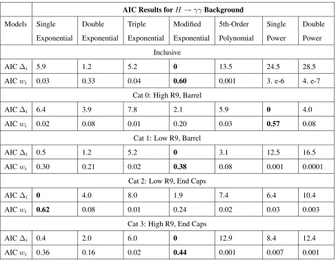
LHC and calculate the AIC weights for each fit model in the model set. The results of this study are displayed in Table 3.2 with the ”best” model for each category in bold. One finds

that the model that is best support most frequently is the modified exponential, as seen in the inclusive, Low R9 Barrel and High R9 End Cap categories. The modified exponential

is also well supported in the other two categories though is preceded by the single power law within the Barrel at High R9 and single exponential in the End Caps at Low R9.

A significant observation to note is that the polynomial fit model was not substantially

supported by the data in any of the five categories. This is contrary to the results of the previous H → γγ background bias study which chose the 5th-Order polynomial as the preferred background model [15, 20]. In Figure 3.4 we display the combined composite model fit to the data for each category along with their likelihoods and the χ2 _{value for}

each fit. We see that each composite model seems to provide an acceptable level of agree-ment within each category. In Table 3.3 we display the rankings of each model based on

(42)

5th order polynomial, double and triple exponential all ranked generally high among the models. However, the discrepancies among the models from the lowest minimized

nega-tive log likelihood reveals that the variations among the few models following the ”best” model by likelihood standard is relatively small. The composite model is included in this

table and ranks consistently around the third or fourth preferred model, with a difference in −2Log(L) < 2.5 for each category. At the very least the composite model for each category provides relatively similar results with the other preferred models.

Plausible Model Set

0. Single Exponential c1eαx

1. Double Exponential c1eαx+c2eβx

2. Triple Exponential c1eαx+c2eβx+c3eγx 3. Modified Exponential c1eαx+η

4. 5th-Order Polynomial c5x5+c4x4+c3x3+c2x2+c1x+c0 5. Single Power Law c1xα

6. Double Power c1xα+c2xβ

(43)

Mass [GeV]

110 120 130 140 150 160 170

Events / ( 0.6 )

0 200 400 600 800 1000 1200 1400 1600 1800 2000 Hgg Background Composite Model -2log(L) : -1325026.334

: 0.968

2 χ

(a) Inclusive Data

Mass [GeV]

110 120 130 140 150 160 170

Events / ( 0.6 )

0 20 40 60 80 100 120 140 160 180 200 220 240 Hgg Background Composite Model -2log(L) : -76836.029

: 0.793 2 χ

(b) Cat 0: Barrel High R9

Mass [GeV]

110 120 130 140 150 160 170

Events / ( 0.6 )

0 100 200 300 400 500 600 700 800 900 Hgg Background Composite Model -2log(L) : -489436.516

: 1.090

2 χ

(c) Cat 1: Barrel Low R9

Mass [GeV]

110 120 130 140 150 160 170

Events / ( 0.6 )

0 20 40 60 80 100 120 140 160 Hgg Background Composite Model -2log(L) : -55972.642

: 1.004

2 χ

(d) Cat 2: Endcaps High R9

Mass [GeV]

110 120 130 140 150 160 170

Events / ( 0.6 )

0 100 200 300 400 500 600 700 800 Hgg Background Composite Model -2log(L) : -472753.942

: 1.005 2 χ

[image:43.612.142.503.140.554.2]

(e) Cat 3: Endcaps Low R9

(44)

AIC Results forH →γγBackground

Models Single

Exponential

Double

Exponential

Triple

Exponential

Modified

Exponential

5th-Order

Polynomial

Single

Power

Double

Power

Inclusive

AIC∆i 5.9 1.2 5.2 0 13.5 24.5 28.5

AICwi 0.03 0.33 0.04 0.60 0.001 3. e-6 4. e-7

Cat 0: High R9, Barrel

AIC∆i 6.4 3.9 7.8 2.1 5.9 0 4.0

AICwi 0.02 0.08 0.01 0.20 0.03 0.57 0.08

Cat 1: Low R9, Barrel

AIC∆i 0.5 1.2 5.2 0 3.1 12.5 16.5

AICwi 0.30 0.21 0.02 0.38 0.08 0.001 0.0001

Cat 2: Low R9, End Caps

AIC∆i 0 4.0 8.0 1.9 7.4 6.4 10.4

AICwi 0.62 0.08 0.01 0.24 0.02 0.03 0.003

Cat 3: High R9, End Caps

AIC∆i 0.4 2.0 6.0 0 12.9 8.4 12.4

[image:44.612.72.559.70.447.2]

AICwi 0.36 0.16 0.02 0.44 0.001 0.007 0.001

(45)

Stability of Model Selection

Want to examine the stability of the MMI process and the consistency of the compos-ite model shape that is produced. In order to assess the stability of the composcompos-ite model

(46)

events. The random selection of events and filling of the new data simulates the statistical variations from one experimental run to another. The MMI method is then run over each

sample and a composite model is produced for each sample.

We evaluate the systematic uncertainty for this composite production by calculating the number of background events within the signal range from 123 GeV to 127 GeV,

nor-malized by the total number of events for each trial, over 800 toy samples. We then fit this distribution with a gaussian to determine the systematic uncertainty of the composite model

production. The measured uncertainty amounts to0.09±0.0002which is well below the statistical uncertainty of 0.31, quoted from the mass measurement of the Higgs boson in the

previousH →γγ analysis [15]. Therefore we determine the consistency of the composite model generation from theH →γγ data to be within acceptable uncertainty.

Constant 101.1 ± 4.8

Mean 0.08928 ± 0.00001

Sigma 0.0002205 ± 0.0000064

0.0870 0.0875 0.088 0.0885 0.089 0.0895 0.09 0.0905 0.091 20

40 60 80 100 120 140

160 Constant 101.1 ± 4.8

Mean 0.08928 ± 0.00001

Sigma 0.0002205 ± 0.0000064

Figure 3.5: Distribution of background events within signal region for composite models derived from 800 toy trials of randomizedH →γγ samples

3.4.2

Bias Analysis

The significance of the model selection for characterizing the Standard Model Background is that an inappropriate function may lead to biased observed signal yields when comparing

(47)

for theH → γγ Standard Model background that minimizes the bias to the signal region. In the previous H → γγ analysis, the method used for selecting a background model was to compare the maximal potential bias that was introduced by each fit model while characterizing possible truth-models. The bias was determined to be, ”the deviation from

zero of the median deviation of the fitted number of mean background events between the truth and the fit-model in a mass window corresponding to the full-width-half-maximum

of the signal model” [7].

Bias(mH) := median NtrueF W HM −Nf itF W HM

(3.4)

One then compares this statistical uncertainty, the value to the uncertainty of the fitted number of events within this region, and define the bias to be negligible when,

median N

F W HM

true −Nf itF W HM

∆NF W HM f it

!

<0.2 (3.5)

In this manner one determines the extent to which each potential fit model alters the ex-pected background event yield within the Higgs signal mass window.

To compare the results from the AIC analysis with this previous study and consider the

potential bias of the composite model, we are replicating this bias study by generating toy events for each possible truth model in the model set and fitting them again with all of the

potential models, including the composite model. By integrating the truth and fit proba-bility density functions within the mass range of 123 to 127GeV /c2_{, weighted by number}

of total events in the toy set, we determine the expected number of background events for the truth and fit models within the bias region. The difference between these is then

(48)

Truth Type Single Exponential

Fit Type Sing.

Exp.

Doub.

Exp.

Trip. Exp Mod.

Exp.

Poly. Sing.

Pow.

Doub.

Pow.

Composite

cat0 0.0033 0.0040 0.0044 0.0041 0.0006 0.0219 0.0219 0.0042

cat1 0.0036 0.0036 0.0036 0.0013 0.0107 0.0214 0.0213 0.0007

cat2 0.012 0.0123 0.0123 0.0233 0.0163 0.0066 0.0066 0.0180

cat3 0.0023 0.0068 0.0054 0.0066 0.0123 0.0176 0.0176 0.0090

cat4 0.0031 0.0031 0.0032 0.0038 0.0004 0.0139 0.0139 0.0033

Table 3.4: Estimated bias of from the various fit models to the signal region of 123 to 127 GeV for the single exponential truth model.

Truth Type Double Exponential

Fit Type Sing.

Exp.

Doub.

Exp.

Trip. Exp Mod.

Exp.

Poly. Sing.

Pow.

Doub.

Pow.

Composite

cat0 0.0221 0.0043 0.0043 0.0076 0.0094 0.0042 0.0005 0.0045

cat1 0.0079 0.0018 0.0039 0.0022 0.0041 0.0093 0.0093 0.0035

cat2 0.0084 0.0084 0.0084 0.0022 0.0178 0.0260 0.0261 0.0074

cat3 0.0033 0.0065 0.0065 0.0071 0.0019 0.0183 0.0183 0.0053

cat4 0.0082 0.0029 0.0028 0.0008 0.0036 0.0082 0.0082 0.0016

Table 3.5: Estimated bias of from the various fit models to the signal region of 123 to 127

(49)

Truth Type Triple Exponential

Fit Type Sing.

Exp.

Doub.

Exp.

Trip. Exp Mod.

Exp.

Poly. Sing.

Pow.

Doub.

Pow.

Composite

cat0 0.0140 0.0048 0.0049 0.0009 0.0118 0.0043 0.0053 0.0036

cat1 0.0100 0.0028 0.0029 0.0073 0.0042 0.0077 0.0078 0.0075

cat2 0.0125 0.0126 0.0126 0.0122 0.0035 0.0319 0.0319 0.0125

cat3 0.0053 0.0025 0.0031 0.0024 0.0053 0.0103 0.0103 0.0041

cat4 0.0001 0.0078 0.0027 0.0041 0.0601 0.0163 0.0163 0.0053

Table 3.6: Estimated bias of from the various fit models to the signal region of 123 to 127 GeV for the triple exponential truth model.

Truth Type Modified Exponential

Fit Type Sing.

Exp.

Doub.

Exp.

Trip.

Exp.

Mod.

Exp.

Poly. Sing.

Pow.

Doub.

Pow.

Composite

cat0 0.0268 0.0079 0.0079 0.0122 0.0111 0.0088 0.0022 0.0088

cat1 0.0050 0.0021 0.0018 0.0000 0.0020 0.0119 0.0119 0.0013

cat2 0.0084 0.0086 0.0084 0.0004 0.0044 0.0276 0.0276 0.0048

cat3 0.0126 0.0058 0.0084 0.0064 0.0050 0.0031 0.0030 0.0072

[image:49.612.107.612.498.665.2]

cat4 0.0114 0.0074 0.0073 0.0057 0.0544 0.0052 0.0052 0.0064

(50)

Truth Type 5th Order Polynomial

Fit Type Sing.

Exp.

Doub.

Exp.

Trip.

Exp.

Mod.

Exp.

Poly. Sing.

Pow.

Doub.

Pow.

Composite

cat0 0.0196 0.0069 0.0069 0.0051 0.0254 0.0018 0.0018 0.0142

cat1 0.0024 0.0002 0.0004 0.0010 0.0120 0.0153 0.0153 0.0118

cat2 0.0008 0.0016 0.0017 0.0017 0.0105 0.0194 0.0194 0.0024

cat3 0.0003 0.0093 0.0027 0.0041 0.0102 0.0149 0.0149 0.0057

cat4 0.0071 0.0022 0.0022 0.0002 0.0001 0.0097 0.0097 0.0007

Table 3.8: Estimated bias of from the various fit models to the signal region of 123 to 127 GeV for the 5th order polynomial truth model.

Truth Type Single Power Law

Fit Type Sing.

Exp.

Doub.

Exp.

Trip.

Exp.

Mod.

Exp.

Poly. Sing.

Pow.

Doub.

Pow.

Composite

cat0 0.0137 0.0044 0.0075 0.0009 0.0121 0.0043 0.0044 0.0047

cat1 0.025 5 0.0114 0.0119 0.0113 0.0056 0.0083 0.0083 0.0091

cat2 0.0105 0.0114 0.0117 0.0038 0.0168 0.0071 0.0074 0.0062

cat3 0.0265 0.0152 0.0159 0.0145 0.0140 0.0120 0.0120 0.0129

cat4 0.0149 0.0059 0.0059 0.0027 0.0048 0.0014 0.0014 0.0035

(51)

Truth Type Double Power Law

Fit Type Sing.

Exp. Doub. Exp. Trip. Exp. Mod. Exp. Poly. Sing. Pow. Doub. Pow. Composite

cat0 0.0126 0.0035 0.0039 0.0026 0.0111 0.0058 0.0059 0.0040

cat1 0.0174 0.0040 0.0043 0.0037 0.0070 0.0009 0.0009 0.0040

cat2 0.0129 0.0097 0.0092 0.0088 0.0091 0.0045 0.0046 0.0088

cat3 0.0193 0.0041 0.0015 0.0072 0.0055 0.0047 0.0033 0.0026

cat4 0.0181 0.0052 0.0039 0.0049 0.0099 0.0021 0.0022 0.0014

Table 3.10: Estimated bias of from the various fit models to the signal region of 123 to 127 GeV for the double power law truth model.

Truth Type Composite Model

Fit Type Sing.

Exp. Doub. Exp. Trip. Exp. Mod. Exp. Poly. Sing. Pow. Doub. Pow. Composite

cat0 0.1338 0.1265 0.1239 0.1241 0.1166 0.1177 0.1175 0.1229

cat1 0.0726 0.0697 0.0705 0.0660 0.0759 0.0561 0.0560 0.0713

cat2 0.0090 0.0299 0.0298 0.0145 0.0552 0.0278 0.0277 0.0304

cat3 0.0222 0.0205 0.0208 0.0205 0.0167 0.0070 0.0070 0.0215

cat4 0.1914 0.1878 0.1879 0.1696 0.1854 0.1776 0.1776 0.1868

Table 3.11: Estimated bias of from the various fit models to the signal region of 123 to 127 GeV for theH →γγ truth model.

3.4.3

Bias in Background Shape and Signal Yield

An additional concern in the model selection is how the shape of the background distribu-tion effects the final locadistribu-tion of the signal peak. Variadistribu-tions in the slope of the background

distribution may lead to biases in the position of the measured signal peak where the mean mass for the Higgs may be shifted to higher or lower values. We examine the variations

(52)

de-termine if there is any substantial variation introduced by the models. Similar to the bias study, the slope for the fit background distribution is determined for each potential fit model

in the set, as well as the composite model, for each potential truth background type. The results for the slopes are displayed in Tabels 3.12 to 3.19.

The composite model, double power law, double and triple exponential models maintain

relatively consistent fit slopes among truth types as well as in relation with each other. The single exponential and polynomial fit models, however, show the greatest variation in

cal-culated slope around the Higgs mass, not only from the other fit models but also among their fits to the various truth models. The deviation in the slope for the polynomial is more

substantial than would be expected and we cannot explain these outcomes. Similarly the values for the single power law fit functions did not converge, despite the fits converging,

which is why they are omitted from the results. Certain categories for the modified expo-nential fits also failed to converge and are designated by a (*). We therefore proceed with

caution in deriving strong conclusions from these results but acknowledge the consistency of the slope resulting from the composite model with the other fit models.

Truth Type Single Exponential

Fit Type Sing Exp Doub Exp Trip Exp Mod Exp Poly Doub Pow Composite

cat0 -0.0007871 -0.0006567 -0.0006584 -0.0006306 -0.0176181 -0.0006935 -0.0006566

cat1 -0.0008828 -0.0006200 -0.0006200 -0.0021350 0.0105560 -0.0006572 -0.0006119

cat2 -0.0007696 -0.0006615 -0.0006615 -0.0036701 -0.0164910 -0.0006984 -0.0006373

cat3 -0.0011159 -0.0005591 -0.0005609 -0.0002608 -0.0154558 -0.0005848 -0.0005314

cat4 -0.0009333 -0.0006031 -0.0006032 -0.0010931 -0.0165993 -0.0006406 -0.0006026

Table 3.12: Estimated slope of various fit models atmH = 125GeV for a single

(53)

Truth Type Double Exponential

Fit Type Sing Exp Doub Exp Trip Exp Mod Exp Poly Doub Pow Composite

cat0 -0.0007432 -0.0007344 -0.0007343 * -0.0184917 -0.0007241 -0.0007176