An Experimental and Quantitative Analysis to Determine the Effect of Changing Inlet Air Temperatures on the Performance of an Oil injected Electrically Powered Twin Screw Air Compressor for Industrial Processes.

Powered Twin Screw Air Compressor for Industrial Processes. (Under the direction of Dr. Stephen Terry.)

The objective of this thesis is to experimentally determine if compressing cooler outside air instead of warm plant air affects the performance of an oil flooded screw compressor. It is common knowledge that compressing cooler air requires less power than compressing warmer air, but the effects of compressing cool air in an oil injected compressor are not known. It is hypothesized that the effect of inlet air temperature on an oil injected screw compressor’s performance will be small since the oil is maintained at specific temperatures.

by

David George Hunt

A thesis submitted to the Graduate Faculty of North Carolina State University

in partial fulfillment of the requirements for the degree of

Master of Science

Mechanical Engineering

Raleigh, North Carolina 2012

APPROVED BY:

_______________________________ ______________________________

Dr. Herbert M Eckerlin Dr. James W Leach

________________________________ Dr. Stephen D Terry

DEDICATION

BIOGRAPHY

David George Hunt was born March 19, 1987 in Oxford, NC. He was raised by two intelligent, inspiring, supportive, hardworking, and loving parents; George and Caroline Hunt. David was raised along with two intelligent and pretty sisters also, Carlyon and Martha Hunt. At the age of six David Hunt moved to Wilson, North Carolina. After high school David moved to Raleigh, North Carolina to study mechanical engineering at North Carolina State University (NCSU).

In college David Hunt quickly discovered earning a degree in mechanical engineering was going to be a rigorous task. Luckily, in college David found a Christian church group and a rugby team to help him with the frustrations of school. Through David’s church group he met a true friend Michael Simon. Michael Simon found David a summer job at the Industrial Assessment Center (IAC). Here David actually enjoyed utilizing his course work to solve real world problems. After 5 years David graduated from NCSU with a bachelor’s of science in mechanical engineering and completed NCSU’s Co-op program.

TABLE OF CONTENTS

LIST OF TABLES ... vi

LIST OF FIGURES ... vii

Chapter 1 – Introduction ... 1

1.1MOTIVATION AND SIGNIFICANCE ... 1

1.2HISTORY ... 2

1.3WHY THEORY IS IMPORTANT ... 8

1.4PRESSURE ... 9

1.5IDEAL GAS OR NOT ... 11

Chapter 2 – Today’s Air Compressor ... 17

2.1THE MODERN COMPRESSED AIR SYSTEM ... 17

2.2PHYSICAL COMPRESSOR OPERATION:RECIPROCATING AND TWIN SCREW ... 20

2.5VOLUMETRIC EFFICIENCY ... 26

2.6EFFICIENT COMPRESSION:ISENTROPIC,POLYTROPIC, OR ISOTHERMAL ... 29

2.6.1 Isentropic Case ... 31

2.6.2 Isothermal ... 36

2.6.3 Polytropic ... 39

2.7AIR PROPERTIES ... 41

2.7.1 Humidity Effect ... 42

2.8THE STANDARD CUBIC FOOT ... 44

2.9THEORY CONCLUSION ... 46

Chapter 3 – Understanding Electricity ... 49

3.1ELECTRICITY AND THREE PHASE POWER ... 49

3.2ACELECTRIC MOTORS ... 54

Chapter 4 – Best Practices ... 61

4.1CAPACITY CONTROL FOR OIL INJECTED SCREW COMPRESSORS ... 61

4.2LOWER COMPRESSOR OUTPUT PRESSURE ... 72

4.3FIX AIR LEAKS ... 75

4.4UTILIZE COMPRESSOR WASTE HEAT ... 83

4.5UTILIZE OUTSIDE AIR ... 86

Chapter 5 – Utilizing Outside Air for Compressor Inlet Temperature Analysis ... 90

5.1HYPOTHESIS AND EXPERIMENTAL OVERVIEW ... 90

5.2THE COMPRESSOR AND OPERATING PARAMETERS ... 94

5.3MEASUREMENT PROCEDURE ... 97

5.4DATA ANALYSIS ... 101

5.4.1 Weekly Data Analysis ... 102

5.4.2 SCFM per Horsepower vs. Inlet Air Temperature ... 108

5.4.3 Input Power vs. Delivered Capacity at Constant Inlet Temperature ... 111

5.4.4 Input Power vs. Inlet Mass at Various Temperatures ... 124

6.1RESULTS AND CONCLUSION ... 132

6.4FUTURE WORK AND SUGGESTIONS ... 137

References ... 139

APPENDICES ... 142

APPENDIX A: CAGI DATASHEET ... 143

APPENDIX B: PACKAGED COMPRESSOR PARTS ... 144

APPENDIX C:PSYCHROMETRIC CHART ... 145

LIST OF TABLES

Table 1: Atmospheric Pressure at Different Altitudes ... 11

Table 2: Steam as an Ideal Gas and Related Error ... 14

Table 3: Generic Leak Rates ... 80

Table 4: Estimated Air Leak Energy Savings ... 82

Table 5: CAGI Highlights in Standard Units ... 95

Table 6: First Week Summary Results ... 105

Table 7: All Weeks Summary Results ... 106

Table 8: Trend Line Power Equations vs. SCFM at Various Temperatures ... 118

Table 9: Predicted Power Differences at Various Temperatures and 396 SCFM ... 122

Table 10: Predicted Horsepower Equations vs. Mass Flow Rate ... 127

LIST OF FIGURES

Figure 1: Originally Three Lobe Blower Design ... 5

Figure 2: Helical Blower Lobes ... 6

Figure 3: Rotary Screw Compressor Screws ... 7

Figure 4: Air Pressure Gauge ... 9

Figure 5: Compressibility Factor vs. Reduced Pressure ... 15

Figure 6: Modern Compressed Air System ... 20

Figure 7: Piston at Top Dead Center ... 21

Figure 8: Cylinder Volume Increasing ... 22

Figure 9: Piston at the Bottom of Stroke ... 22

Figure 10: Piston at Top Dead Center Again ... 23

Figure 11: Reciprocating Compressor Full Cycle ... 24

Figure 12: Compressor Screws ... 25

Figure 13: Volumetric Efficiency vs. Pressure Ratio for Reciprocating Compressor ... 28

Figure 14: Thermodynamic Air Compressor Diagram ... 30

Figure 15: Compression Processes Pressure vs. Specific Volume ... 40

Figure 16: Oil Free Screw Compressor Volumetric and Adiabatic eff. vs. Inlet Pressure ... 47

Figure 17: Oil Flooded Screw Compressor Volumetric and Adiabatic eff. vs. Discharge Pressure ... 47

Figure 18: Compressed Air System Control Volume ... 48

Figure 19: Three Phase Power ... 50

Figure 20: Three Phase Four Wire Wye ... 52

Figure 21: Three Phase Wire Delta ... 53

Figure 22: Three Phase Two Wire Corner-Grounded Delta ... 53

Figure 23: Characteristic Curve for an Electric Motor ... 56

Figure 24: Motor Heating Curve... 57

Figure 25: Motor Efficiency vs. Percent Full Load ... 58

Figure 26: Electricity Leading and Lagging ... 58

Figure 28: Oil Injected Screw Compressor Modulating Power vs. Capacity ... 63

Figure 29: Screw Compressor, Oil Separator, and After Coolers ... 65

Figure 30: Oil Injected Screw Compressor with Blowdown Power vs. Capacity ... 66

Figure 31: Load Unload Capacity Control... 67

Figure 32: Variable Displacement Percent Power vs. Capacity ... 69

Figure 33: Power vs. Capacity Using a VFD Screw Compressor ... 70

Figure 34: Swing Compressor Operation ... 71

Figure 35: Oil Flooded Screw Compressor Diagram ... 91

Figure 36: Packaged Air Compressor ... 95

Figure 37: Current Transformer ... 97

Figure 38: Inlet Temperature Probe ... 98

Figure 39: Flow Meter ... 99

Figure 40: H22 Energy Logger ... 100

Figure 41: RH Meter ... 100

Figure 42: Data Measurement Diagram ... 101

Figure 43: First Week Compressor Data ... 103

Figure 44: Average Horsepower versus Average Temperature ... 107

Figure 45: SCFM /hp vs. Inlet Air Temperature Averaged Over 3 Minutes ... 109

Figure 46: SCFM /hp vs. Inlet Air Temperature Averaged Over 30 Minutes ... 110

Figure 47: Hypothesized Horsepower vs. SCFM Plot if Temperature Affects Power ... 111

Figure 48: Horsepower vs. Flow All Weeks ... 113

Figure 49: Horsepower vs. SCFM at Various Temperatures ... 117

Figure 50: Predicted Horsepower vs. Delivered Flow at Various Temperatures ... 120

Figure 51: Predicted Horsepower vs. Delivered Flow at Various Temperatures Zoomed In121 Figure 52: Percent Power Increase vs. Inlet Air Temperature ... 123

Figure 53: Horsepower vs. Inlet Mass Flow Rate... 126

Figure 54: Horsepower vs. Mass Flow Rate ... 128

Figure 55: Horsepower vs. Mass Flow Rate Zoomed In ... 129

Chapter 1 – Introduction

1.1 Motivation and Significance

The total amount of electrical energy consumed in the United States was 3,884 Billion kWh in 2010 (1). Experts, in the United States of America, estimate 26% of electricity generated is consumed by industry and 10% of the electricity utilized in industry is devoted to

generating compressed air (2). Therefore 101 billion kWh of energy were devoted to generating compressed air in the year of 2010. To put this phenomenal amount of energy in prospective it would take all the nuclear power plants in North Carolina operating fully loaded nonstop for 2.32 years to generate this amount of energy. With substantial numbers like this it should be obvious generation of compressed air needs to be as efficient as possible.

strong focus on inlet air temperatures is addressed to determine whether inlet air temperatures affect oil flooded screw compressors or not.

This study will consider if an oil flooded screw compressor consumes less energy using outside air rather than warmer plant air. Currently there is confusion on this topic because some energy engineers recommend using outside air in oil flooded screw compressors. If this recommendation is wrong then industrial facilities need to be educated so they will stop wasting money on useless energy savings projects and focus their time and money on proven applications or technologies.

1.2 History

resides in human lungs a biological process occurs. Red blood cells release carbon dioxide while capturing oxygen from the air. Carbon dioxide fills the lungs and the fresh oxygen is sent to other body parts such as the heart and brain. The carbon dioxide must leave the lungs because it is a poisonous to the human body. Carbon dioxide is removed by contracting the lungs or decreasing the volume of space the lungs occupy. This compresses the carbon dioxide inside the lungs. Once the carbon dioxide’s pressure, due to compression, is greater than the surrounding atmosphere it exits the lung due to a pressure differential.

Understanding this explains why it is harder to breath at higher altitudes. For example atmospheric pressure is 14.696 pounds per square inch atmospheric (psia) at sea level while a top Mount Everest, a little under 30,000 feet, the atmospheric pressure is roughly 4.371 psia (3). There is a smaller pressure differential on top Mount Everest than sea level, because of a smaller pressure differential air does not enter the lungs easily on top Everest.

stroke and sealed the cylinder on the compression stroke. More advanced piston devices were used by the Greeks around 150 BC (6). These piston cylinder devices were made of metal. As metallurgy advanced more compressed air was needed therefore larger more efficient bellows were needed. Eventually people discovered the energy potential of water (hydro power) and used it to operate larger bellows. Examples of large water powered bellows can be seen at historical blacksmith shops around the country (4).

Compressed air became such a reliable muscle for work that engineers started playing with the idea of using it as a viable energy source in the early 1800’s (4). At this time steam was widely used to power industrial devices, but steam was a messy and dangerous energy source that was hard to transmit over long distances. Therefore compressed air seemed very

The mining industries drastically changed compressed air. Lightweight pneumatic drills and hammers allowed miners to move through rock faster than ever, which truly showed the reliability of compressed air to perform work. Mining not only advanced compressed air tools but also paved the path for the screw compressor used today. In 1854 the Roots blower was invented by the Roots brothers (6). The Roots blower was initially designed to remove water from mines by pumping it. Unfortunately the blower was not very successful at this task and was adjusted for air and gas compression. A patent of the Roots blower was made in 1860 (5) (6). The patented Roots blower boosted gas for furnaces and ventilated mines for miners. In 1878, Krigar expanded on the Roots blower design and designed an advanced blower that utilized helical lobes (6). Figure 1 below shows the original lobe design for a Roots blower and Figure 2 below shows the helical blower lobe design.

Figure 2: Helical Blower Lobes (7)

Originally compressed air was not easily available to everyone because it required a substantial power source usually in the form of steam which only large companies could afford. In the 1900’s packaged compressed air units that utilized electricity were being produced because advancements in electrical power distributions and electrical motors were made (4). Packaged compressors were great for most businesses that desired a reliable robust energy source because they had access to electrical power now. As packaged compressed air units were produced more pneumatic tools were produced driving down the cost of pneumatic tools. Pneumatic tools were great because they are reliable and they helped manufactures increase production rates. During World War II anything that could increase production was embraced, thus, compressed air was embraced and proved its reliability once again (4).

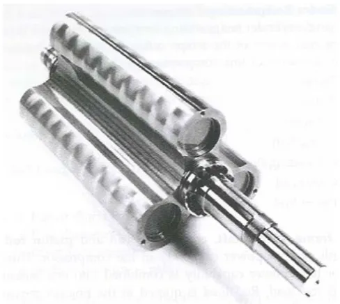
gas turbine in the 1930’s. Lysholm needed a compressor that used a rotating action at high speeds that could not surge. Therefore Lysholm developed the twin screw compressor using the 1878 helical blower design by Krigar (6). Lysholm’s twin screw compressor could not supply the volume of air his turbine needed at a practical size. Even though the twin screw compressor did not do what Lyshom wanted a Swedish research group Svenska Rotor Maskiner developed the idea of using the twin screw compressor for industrial applications (6). In 1946 companies started using the twin screw compressor. Industrial twin screw compressors utilized an oil free design until 1957 when the first oil injected machine hit the market (6). Oil free means zero particles of oil in the air stream that is compressed and oil flooded means oil particles are injected into the compressor’s inlet, along with air, as air is compressed. 40 to 500 horsepower compressor are most common sizes today (4). A set of screw compressor screws is shown in Figure 3 below.

1.3 Why Theory is Important

Predicting how much energy is consumed by an air compressor is a useful tool to anybody that uses compressed air. Unfortunately predicting energy consumption can be difficult because both practical and theoretical knowledge is needed. Theoretical knowledge demonstrates why compressed air is energy intensive. Plus modifying a compressor in theory, on a piece of paper, is easier than modifying one in the real world. For example, take a plant engineer who spends a large sum of money to modify his air compressor to accept outside air in the winter months. With these modifications there is an expectation of a quick payback to the investment. If the fast payback period is not achieved, then reputations are damaged and other energy conservation measures are questioned. A situation such as this could be avoided by first testing the modification on paper with a thorough understanding of the physics. If desired results are found on paper then they should be implemented.

1.4 Pressure

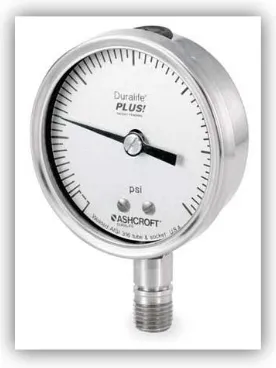
Pressure is defined as a normal force exerted by a fluid per unit area (8). This is a simple concept yet there are so many different ways to represent units of pressure it makes pressure confusing. For example when calculating compressor performance absolute pressure must be used but in industry pressure may be referred to in one of the following ways, pound force per square inch (psi), pound force per square inch gauge (psig), pound force per square inch absolute (psia), or pound force per square inch differential (psid). Most commonly pressure is referred to in units of psi. Pressure is referred to in psi most commonly because most gauges report in psi, see Figure 4.

Figure 4: Air Pressure Gauge (9)

measured relative to a vacuum with absolute zero pressure. Most pressure gauges are calibrated to measure zero at atmospheric conditions. Therefore when a pressure gauge is read on a car tire or compressed air pipe the atmospheric pressure needs to be added to the gauge pressure to know absolute pressure inside the tire or pipe. This is analytically written as follows:

𝑃𝑎𝑏𝑠𝑜𝑙𝑢𝑡𝑒 = 𝑃𝑔𝑢𝑎𝑔𝑒+ 𝑃𝑎𝑡𝑚𝑜𝑠𝑝ℎ𝑒𝑟𝑒 (Eqn. 1.4.1)

Most of the time it is safe to assume atmospheric pressure is 14.7 psia, but atmospheric pressure does vary with altitudes. Atmospheric pressure is greatest towards the center of earth because the atmosphere gets denser as you approach the center. It is like swimming in a pool, as you approach the bottom of the pool you feel a greater force exerted on your body due to an increasing pressure. This is because the weight of water molecules stacked on top of each other increases with depth. This example can be expressed with the following equation for pressure:

𝑃𝑎𝑏𝑠𝑜𝑙𝑢𝑡𝑒 = 𝜌𝑔ℎ (Eqn. 1.4.2)

Where,

P = Pressure 𝜌 = Density of fluid

g = Gravitational constant at location h = Height from desired location of pressure

is 121,894,000 pounds force. The following table shows variations of atmospheric pressure with altitude.

Table 1: Atmospheric Pressure at Different Altitudes (10)

1.5 Ideal Gas or Not

Probably the most common and most misused equation relating pressure, volume, and temperature is the ideal gas equation of state. This famous equation is commonly written as follows:

Pv = RT (Eqn 1.5.1)

Where,

R = Gas constant for a particular gas (BTU/lbm-R) T = Absolute temperature (R)

Note R can be found for any gas as follows:

R = Ru / M (Eqn. 1.5.2)

Where,

Ru = Universal gas constant (1.98588 BTU/lbmol-R)

M = Molecular weight of particular gas (lbm/lbmol)

This equation is commonly misused because, in reality, a truly ideal gas does not exist. However, under the right conditions it is safe to assume a gas is ideal with little error. A compressibility factor was created to show how ideal a gas is. The compressibility factor is represented by the letter Z and found with the following equation:

𝑍= 𝑣𝑎𝑐𝑡𝑢𝑎𝑙 _𝑣 𝑖𝑑𝑒𝑎𝑙

� (Eqn. 1.5.3)

Where,

vacutal = Actual specific volume of gas (ft3/lbm)

videal = ideal specific volume of gas (ft3/lbm) = RT/P

Now evaluate steam at another temperature and pressure, 200 psia and 381.8ºF. At this state steam tables give an actual specific volume of 2.2882 ft3/lbm. Assuming steam is an ideal gas at this state gives an ideal specific gas volume of 2.507 ft3/lbm. Steam does not deviate from the ideal gas assumption much. The compressibility factor for this example is 1.15 with a percent error of 13.0%.

Evaluate steam as ideal gas at a pressure of 3,200.1 psia and 705ºF. Note this is nearly the critical pressure (3,200 psia) and temperature (704.8ºF) of water. The actual specific volume of steam at this state is 0.04975 ft3/lbm. Using the ideal gas assumption the ideal specific volume of steam is 0.217 ft3/lbm. The compressibility factor for this example is 0.229 with a percent error of 336%. It is fairly obvious using the ideal gas assumption for steam around this temperature and pressure will result in significant error.

To realize when a gas is approaching its critical point two unitless normalizations were created. The reduced pressure (Pr) and reduced temperature (Tr). These normalizations are

found as follows:

Pr = Pactual / Pcritical (Eqn. 1.5.4)

Tr = Tactual / Tcritical (Eqn. 1.5.5)

To demonstrate the benefits from normalizing pressure and temperature with their critical points consider the example of steam given earlier. Below in Table 2, reduced temperature and pressure are reported. Two states of steam are added to the example given earlier also.

Table 2: Steam as an Ideal Gas and Related Error

State

Actual Temp. (ºF)

Tr

Actual Pressure

(psia)

Pr

vactual

(ft3/lbm)

videal

(ft3/lbm) Z Error

1 102 0.482 1 0.00 333 335 0.997 0.32%

2 382 0.723 200 0.06 2.88 2.51 1.15 13%

3 518 0.840 800 0.25 0.569 0.73 0.78 28%

4 705 1.00 3,200 1.00 0.050 0.22 0.23 336% 5 2,000 2.11 3,000 0.94 0.485 0.488 0.99 1%

the error associated with assuming steam is ideal, 1%. Table 2 shows as the reduced temperature and pressure approach one, the critical point, the error assuming ideal gas increases drastically. State three has an error of 28% and state four has an error of 336%.

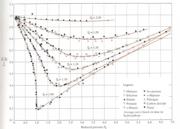
Researchers have created plots to support this evidence with experimentally determined Z values plotted against reduced pressure and reduced temperature. Figure 5 is a plot of reduced temperature, reduced pressure, and experimentally determined compressibility factors for several different gases.

Figure 5: Compressibility Factor vs. Reduced Pressure (8)

In conclusion it is safe to assume a gas is ideal when its pressure is very low (Pr <<1), when

extremely high (Tr >>1). It is important to understand that a gas deviates from the ideal gas

Chapter 2 – Today’s Air Compressor

2.1 The Modern Compressed Air System

In the past compressed air was used to feed fires and today its common knowledge

compressors are energy hogs, thus, why is compressed air still used today? Compressed air is very valuable to industrial facilities today because of its power and reliability.

Compressed air is commonly used to operate tools such as impact wrenches, drills, and grinders. More efficient electrical motors could be used to power these tools but they are heavy and cause people, such as plant employees, to fatigue over time. Fatigue is not good because it can decreases production. To show the difference between an electric tool and a pneumatic tool the power to weight ratio for a grinder can be compared. The power to weight ratio of random electric grinder is 0.09 horsepower per pound while a pneumatic grinder is 0.31 horsepower per pound (4). The compressed air tool is nearly three and half times more powerful per pound!

Compressed air is commonly used for process controls today also. For particular

To make sure pneumatic tools and or controls operate reliably and efficiently they must have a reliable source of compressed air. The most important device to supply compressed air is an air compressor. An air compressor compresses air from atmospheric pressure to an elevated pressure. When air expands from an elevated pressure to atmospheric pressure it can be used to do work or operate several pneumatic tools like the ones mentioned above. There are several different types of air compressor for different applications. It is very important to choose the correct air compressor depending on the task needed.

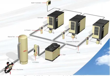
Storing high pressure air is essentially storing energy. Commonly a receiver, usually in the shape of a tank, is installed in a compressed air system to store compressed air. A receiver is an essential part to a compressed air system because it keeps system pressure consistent and it acts as a buffer. Consistency is important because many pneumatic tools, controls, and process require a particular pressure. When a receiver acts as a buffer it allows a compressor to unload more often. An unloaded compressor will consume less energy than a loaded compressor.

Air commonly has moisture in it that needs to be removed before it is used in tools and or process. An air dryer is a device used to remove moisture in a stream of compressed air. Two types of air dryers are commonly used a refrigerant type and desiccant type. The refrigerant air dryer utilizes a vapor compression cycle to condense and remove moisture. The desiccant dryer utilizes compressed air and a desiccant to remove moisture. The desiccant dryer consumes more energy but removes more moisture. Selecting a dryer depends on what the compressed air is used for.

Figure 6: Modern Compressed Air System (11)

2.2 Physical Compressor Operation: Reciprocating and Twin Screw

Figure 7: Piston at Top Dead Center

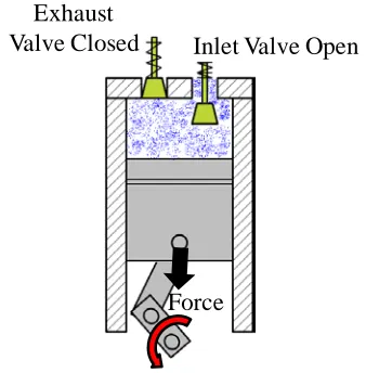
A force is applied to the piston to pull it down. As the piston is pulled down the cylinder’s volume increases creating a vacuum inside the cylinder. Atmospheric pressure on top the valve is greater than gauge pressure inside the cylinder. This pressure differential causes the intake valve to open and causes air to fill the cylinder (i.e. blue dots represent air in Figure 8).

Clearance Volume

Inlet Valve Exhaust Valve

Piston

Figure 8: Cylinder Volume Increasing

Once the piston is at the bottom of its stroke, the largest volume of the cylinder, it is pushed back up by an external force.

Figure 9: Piston at the Bottom of Stroke

Force

Inlet Valve Open Exhaust

Valve Closed

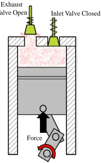
As the piston moves towards top dead center the cylinder’s volume decreases and pressure increases. According to the ideal gas law, equation 1.5.1 above, as volume decreases the pressure increases. Once the pressure inside the cylinder is greater than atmospheric pressure the intake valve closes. The exhaust valve opens once a desired pressure inside the cylinder is met. Usually the predetermined pressure is controlled by a spring forcing the valve shut. Using different spring rates or adjusting how much the spring is compressed allows the compressors operator to adjust the compressors outlet pressure. As the exhaust valve opens compressed air is released from the piston cylinder device.

Figure 10: Piston at Top Dead Center Again

Note compressed air is represented with red dots in Figure 10 because compressing air generates heat. Once the piston reaches top dead center again most the compressed air has been pushed out the cylinder and both the intake and exhaust valve are closed and the cycle is ready to repeat. Today, the force to drive the piston is most commonly done with an

Force

Inlet Valve Closed Exhaust

electric motor. In the past, steam was used to generate this force. Below, Figure 11, shows nearly a complete cycle.

Figure 11: Reciprocating Compressor Full Cycle

A disadvantage to the reciprocating compressor is it’s up and down motion causes vibration. Therefore a reciprocating compressor must be mounted on a secure platform or it will vibrate so much it fails over time.

This air at a higher pressure (compressed state) is the compressor’s objective because compressed air can be used to drive robust tools such as drills.

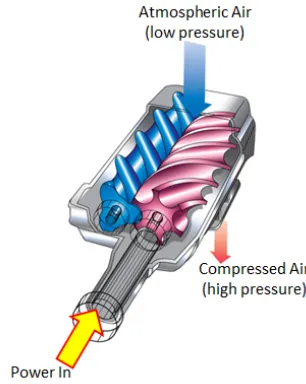
One of the most common compressor found in the manufacturing world today is the twin screw compressor, commonly referred to as the screw compressor. The screw compressor does not compress air as shown above. However, the screw compressor in principle compresses air the same way, via mechanically shrinking a volume of air. The most basic screw compressor has two screws, a male and female, and a case. Below, Figure 12, shows the male screw (left) and female screw (right) meshed together.

Figure 12: Compressor Screws (12)

as the screws rotate they compress the air against the screw’s housing. The air compresses because of the screws conical taper (12). Once the air is at the end of the screws it is discharged. An advantage of the screw compressor is its ability to compress air with a coolant, such as oil. The coolant removes heat during the compression process, lubricates screws, and ensures meshing of screws. Another advantage of the screw compressor is its rotational operation. This allows the compressor to be mounted anywhere. Unlike the reciprocating compressor, vibration is less of an issue with the screw compressor. This also means less maintenance.

Both the compression process above are completed with positive displacement compressors. Another way to compress gases is using a dynamic compressor. Dynamic compressor work using a fluid’s kinetic energy to compress itself against the compressor housing. Dynamic compressors are not seen as often as positive displacement compressors therefore will not be discussed further.

2.5 Volumetric Efficiency

compressor (6). This means if the volume of air drawn into a reciprocating or screw compressor is measured and the volume of air discharged out the compressor is measured and converted back to inlet conditions the values would differ. An easier way to understand volumetric efficiency maybe stating: the mass of air exiting the discharge port of a

compressor is smaller than the mass of entering the suction port.

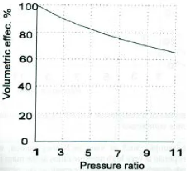
The greatest effect on volumetric efficiency, for reciprocating compressors, is clearance volume. During a compressor’s compression stroke some of the compressed air does not leave the compressor but instead occupies the compressor’s clearance volume. Note air left in the clearance volume is around the compressor’s discharge pressure. When the

compressor begins its suction stroke the air occupying the clearance volume expands and keeps the inlet valve from opening until the cylinders pressure drops below that of atmosphere. This limits the amount of air the compressor can draw in during its suction stroke, thus, the volume of air discharged is smaller than the cylinder’s volume. The greater a compressors discharge pressure ratio the lower its volumetric efficiency. The reason being higher discharge pressure means higher pressure air occupies the clearance volume.

Therefore it takes longer for the cylinders internal pressure to drop below that of atmosphere. The other factors that lead to a reciprocating compressors volumetric efficiency are

and cylinder wall without being compressed. A plot of volumetric efficiency versus pressure ratio is shown below in Figure 13

Figure 13: Volumetric Efficiency vs. Pressure Ratio for Reciprocating Compressor (6)

force for air to escape. Plots of volumetric efficiency versus pressure ratio (Figure 16 and Figure 17) for screw compressors are found in Section 2.9.

2.6 Efficient Compression: Isentropic, Polytropic, or Isothermal

When a system goes from one equilibrium state to another it is considered a process. The act of compressing air is a process because air goes from a one state to another, usually a state of low pressure at some temperature to a state of high pressure at an elevated temperature. There are three different process paths air can follow as it is compressed. In particular air can be compressed using an isentropic process or an isothermal process. In actuality air is compressed in a polytropic process. Understanding all three processes is important because they clarify how compressors work in the physical world and help predict how much energy is consumed by a compressor.

compressibility factor of nearly one no matter the reduced pressure. The maximum reduced pressure will be 0.26 for every case. The following diagram will be used when calculating compressor energy requirements.

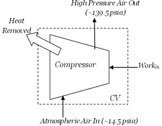
Figure 14: Thermodynamic Air Compressor Diagram

The following symbols will be used during derivations:

ΔE𝐶𝑉 = change in rate of energy of control volume (BTU/hr)

E𝑖𝑛 𝑡𝑜𝐶𝑉 = rate of energy into control volume (BTU/hr)

E𝑜𝑢𝑡 𝑜𝑓𝐶𝑉 = rate of energy out of control volume (BTU/hr)

𝑄𝑖𝑛 = rate of heat into control volume (BTU/hr)

𝑄𝑜𝑢𝑡 = rate of heat out of control volume (BTU/hr)

m1 = mass flow rate of air entering control volume (lbm/hr)

h1 = enthalpy of air entering control volume (BTU/lbm)

h2 = enthalpy of air exiting control volume (BTU/lbm)

2.6.1 Isentropic Case

An isentropic compressor is a steady flow, reversible and adiabatic device (i.e. heat is not removed from the air being compressed) where kinetic and potential energy changes can be neglected meaning no entropy will be generated. Air will also be assumed to have constant specific heats and to be an ideal gas. Using these assumptions and the control volume in Figure 14 the work required to compress air from 14.5 psia at 68ºF to 139.5 psia is found as follows:

ΔE𝐶𝑉 = 0

E𝑖𝑛 𝑡𝑜𝐶𝑉 = E𝑜𝑢𝑡 𝑜𝑓𝐶𝑉

W𝑖𝑛 + m1 (ℎ1) = m2(ℎ1)

For a steady flow device the mass entering must equal the mass leaving, therefore:

W𝑖𝑛 = [𝑚(ℎ2− ℎ1)] ∙ 𝐶 (Eqn. 2.6.1)

For an ideal gas enthalpy is a function of temperature only. Therefore equation 2.6.1 can be rewritten as:

W𝑖𝑛 = 𝑚 ∙ 𝑐𝑝∙(𝑇2− 𝑇1) ∙ 𝐶 (Eqn. 2.6.2)

Where,

Win = Rate of energy or power required to compress air (BTU/hr)

T2 = Temperature of air leaving compressor (ºF)

cp = Specific heat of air at constant pressure (BTU/lbm-ºF)

C = Conversion constant, (1 hp-hr/2,545 BTU)

Equation 2.6.2 will predict the amount of horsepower required to compress 690 CFM of air from 14.5 psia to 139.5 psia. One problem exists with equation 2.6.2, the outlet temperature of the compressor is not known. This outlet temperature could be measured but this can be difficult to do. Assuming air is compressed isentropically the outlet temperature can be found theoretically from one of the three isentropic relationships. For an ideal gas with constant specific heats the following equations can be derived:

𝑠2 − 𝑠1 =𝑐𝑣𝑙𝑛 �_𝑇𝑇2₁�+𝑅𝑙𝑛 �𝑣_𝑣2₁� (Eqn. 2.6.3)

𝑠2− 𝑠1 = 𝑐𝑝𝑙𝑛 �_𝑇𝑇2₁� − 𝑅𝑙𝑛 �𝑃_𝑃2₁� (Eqn. 2.6.4)

Where,

s2 = Entropy leaving the compressor (BTU/lbm-R)

s1 = Entropy entering the compressor (BTU/lbm-R)

cv = Specific heat of air at constant volume (BTU/lbm-ºF)

R = Gas constant for air (BTU/lbm-R)

P2 = Absolute pressure of air exiting the compressor (psia)

P1 = Absolute pressure of air entering the compressor (psia)

v1 = Specific volume of air entering the compressor (ft3/lbm)

Isentropic means no entropy is generated, therefore (s2-s1 = 0). Using the isentropic

assumption and algebra each equation can be rearranged as follows:

�𝑇2

𝑇1�=�

𝑣1

𝑣2�

𝑅 𝑐�𝑣

(Eqn. 2.6.5)

�𝑇2

𝑇1�=�

𝑃2

𝑃1�

𝑅 𝑐�𝑝

(Eqn. 2.6.6)

Equations 2.6.5 and 2.6.6 are fine to use, but in many thermodynamic books these equations are rearrange to look as follows:

�𝑇2

𝑇1�=�

𝑣1

𝑣2�

(𝑘−1)

(Eqn. 2.6.7)

�𝑇2

𝑇1�=�

𝑃2

𝑃1�

(𝑘−1) 𝑘 �

(Eqn. 2.6.8)

Equations 2.6.7 and 2.6.8 are found knowing:

R = cp - cv (Eqn. 2.6.9)

and,

k = cp / cv (Eqn. 2.6.10)

What most thermodynamic books do not show is how to get from equations 2.6.5 and 2.6.6 to equations 2.6.7 and 2.6.8. To get from equation 2.6.5 to 2.6.7 simply plug equation 2.6.9 into equation 2.6.5 as follows:

�𝑇_𝑇2

1�= �

𝑣1

𝑣2�

(𝑐𝑝 − 𝑐𝑣) 𝑐𝑣

�

𝑐𝑝

𝑐𝑣 −

𝑐𝑣

𝑐𝑣 = (𝑘 −1)

and the final result is equation 2.6.7. There is a special trick to finding equation 2.6.8 from 2.6.6. The trick is to multiply the exponent in equation 2.6.6 by a ratio equivalent to one as follows:

𝑅 𝑐𝑝∙1 =

𝑅 𝑐𝑝∙ � 1 _𝑐 𝑣 � 1 _𝑐 𝑣 � �= 𝑅 𝑐� 𝑣 𝑐𝑝 𝑐𝑣 � = (𝑐𝑝 − 𝑐𝑣) 𝑐𝑣 � 𝑘 =

(𝑘 −1)

𝑘

Finally equation 2.6.8 is found. Using equations 2.6.7 and 2.6.8 is easier than 2.6.5 and 2.6.6 because fewer variables have to be found. Looking at equations 2.6.7 and 2.6.8 there is a third relationship that can be found.

�𝑃2

𝑃1�= �

𝑣1

𝑣2�

𝑘

(Eqn. 2.6.11)

Equations 2.6.7, 2.6.8, and 2.6.11 are known as the isentropic relationships. It must be remembered when using these equations the system is assumed to be isentropic therefore no entropy is generated. In reality this will never occur because it is never a totally reversible process.

Back to the original problem, equation 2.6.2 could not be solved because the outlet temperature of air leaving the compressor was not known. Rearranging equation 2.6.8 to find T2, inserting it into equation 2.6.2, and including the conversion from Fahrenheit to

W𝑖𝑛 = 𝑚 ∙ 𝑐𝑝∙(𝑇1+ 460)∙ ��𝑃_𝑃2₁� (𝑘−1)

𝑘 �

−1� ∙ 𝐶 (Eqn. 2.6.12)

To remove the cp in equation 2.6.12 another trick is needed. Both sides of this equation need

to be multiplied by R/R, which equal 1. Using algebra the following is found:

�W𝑖𝑛 = 𝑚 ∙ 𝑐𝑝∙(𝑇1+ 460)∙ ��𝑃_𝑃2 1�

(𝑘−1) 𝑘 �

−1� ∙ 𝐶�𝑅_𝑅

W𝑖𝑛 = 𝑚 ∙𝑐_{𝑅 ∙ 𝑅 ∙}𝑝 (𝑇1+ 460)∙ ��𝑃_𝑃2 1�

(𝑘−1) 𝑘 �

−1� ∙ 𝐶

Where,

𝑐𝑝

𝑅 = 𝑘 𝑘 −1

Therefore equation 2.6.12 can be re written as:

W𝑖𝑛 = 𝑚 ∙_𝑘−1𝑘 ∙ 𝑅 ∙(𝑇1+ 460)∙ ��𝑃_𝑃2₁� (𝑘−1)

𝑘 �

−1� ∙ 𝐶 (Eqn. 2.6.13)

Another variable is still unknown, (m) the mass flow rate. The mass flow rate of air is fairly simple to determine with the following equation:

𝑚= 𝐶𝐹𝑀 ∙ 𝜌 ∙60 (Eqn. 2.6.14)

Where,

CFM = volumetric flow into the compressor (ft3/min) 𝜌 = density of air at inlet conditions (lbm/ ft3)

Finally the equation to find the isentropic work required to compress air adiabatically at a constant flow rate assuming air is an ideal gas with constant specific heats is:

W𝑖𝑛 = 𝐶𝐹𝑀 ∙ 𝜌 ∙60∙_𝑘−1𝑘 ∙ 𝑅 ∙(𝑇1+ 460)∙ ��𝑃_𝑃2₁� (𝑘−1)

𝑘 �

−1� ∙ 𝐶 (Eqn. 2.6.15)

In reality a 150 horsepower compressor is need to compress 690 CFM of air from 14.5 psia to 139.5 psia. Equation 2.6.15 predicts the following:

W𝑖𝑛 = 690∙0.074∙60∙_1.41.4₋₁∙0.06855∙(68 + 460)��139.5_14.5� (1.4−1)

1.4 �

−1� ∙_2,5451

W𝑖𝑛 = 139 ℎ𝑜𝑟𝑠𝑒𝑝𝑜𝑤𝑒𝑟

The isentropic power required to compress air is lower than the actual power required. An isentropic process is ideal; it assumes no entropy generation therefore there are no losses (i.e. friction). An isentropic efficiency needs to be included to calculate the actual power required to compress air at the given conditions. The isentropic efficiency of a compressor is defined as:

𝜂𝑖𝑠𝑒𝑛𝑡𝑟𝑜𝑝𝑖𝑐 = W_W𝑖𝑠𝑒𝑛𝑡𝑟𝑜𝑝𝑖𝑐_{𝑎𝑐𝑡𝑢𝑎𝑙} (Eqn. 2.6.16)

2.6.2 Isothermal

all the heat is removed from air during the compression process? Logically thinking the compressor will require less power to compress air. As temperature rises, air expands (ideal gas law) equation 1.5.1. Therefore in the adiabatic process above the compressor is fighting expansion of air as its temperature rises. If the temperature is held constant (isothermal) the compressor will not have to fight the expanding air.

Assume the compressor is a steady flow non-adiabatic device where all the heat is removed during the compression process, where kinetic and potential energy can be neglected. Also, assume air has constant specific heats and an ideal gas. Using these assumptions and the control volume for a compressor, shown in Figure 14, the work required to compress air from 14.5 psia at 68ºF to 139.5 psia is found as follows:

ΔE𝐶𝑉 = 0

E𝑖𝑛 𝑡𝑜𝐶𝑉 = E𝑜𝑢𝑡 𝑜𝑓𝐶𝑉

W𝑖𝑛 + m1 (ℎ1) =𝑄𝑜𝑢𝑡 + m2(ℎ2)

For a steady flow device the mass entering must equal the mass leaving, therefore:

W𝑖𝑛 = [𝑄𝑜𝑢𝑡+𝑚(ℎ2− ℎ1)] ∙ 𝐶 (Eqn. 2.6.17)

Finally another assumption should be made. Assume the work done in this process is quasi-equilibrium. Since the work done is quasi-equilibrium it is also reversible work in theory. Net heat transfer from an internally reversible process is defined as:

Q𝑖𝑛𝑡.𝑟𝑒𝑣 =∫ 𝑇₁2 d𝑆 (Eqn. 2.6.18)

𝑇 ∙ 𝑑𝑆=𝑑𝐻 − 𝑉𝑑𝑃 (Eqn. 2.6.19) Equation 2.6.17 can be rewritten as follows:

𝑊𝑖𝑛 = [−𝑄𝑖𝑛𝑡.𝑟𝑒𝑣+𝑚(ℎ2− ℎ1)] ∙ 𝐶 (Eqn. 2.6.20)

𝑊𝑖𝑛 = �−𝑚 ∫ 𝑇𝑑𝑠₁2 +𝑚(ℎ2− ℎ1)� ∙ 𝐶 (Eqn. 2.6.21)

𝑊𝑖𝑛 = �−𝑚 ∫ 𝑑ℎ₁2 +𝑚 ∫ 𝑣𝑑𝑃₁2 +𝑚(ℎ2− ℎ1)� ∙ 𝐶 (Eqn. 2.6.22)

𝑊𝑖𝑛 = �𝑚 ∫ 𝑣𝑑𝑃₁2 � ∙ 𝐶 (Eqn. 2.6.23)

To find the power needed to compress air, specific volume (v) as a function of pressure needs to be known. Since air is assumed to be an ideal gas rearranging the ideal gas equation (equation 1.5.1) and plugging it into equation 2.6.23 can be done as follows:

𝑊𝑖𝑛 = �𝑚 ∫₁2𝑅(𝑇1+460)_𝑃 𝑑𝑃� ∙ 𝐶 (Eqn. 2.6.24)

Integrating equation 2.6.24 gives the following:

𝑊𝑖𝑛 = 𝑚𝑅(𝑇1+ 460)𝑙𝑛 �𝑃_𝑃2₁� ∙ 𝐶 (Eqn. 2.6.25)

Inserting equation 2.6.14 for mass flow rate the following is found:

𝑊𝑖𝑛 = 𝐶𝐹𝑀 ∙ 𝜌 ∙60∙ 𝑅 ∙(𝑇1+ 460)∙ 𝑙𝑛 �𝑃_𝑃2₁� ∙ 𝐶 (Eqn. 2.6.26)

Equation 2.6.26 represents, analytically, how much power is required to compress air from a low pressure to an elevated pressure assuming the process is isothermal, the gas is ideal, and specific heats are constant. The amount of power required to compress 690 CFM into the compressor at 68ºF from 14.5 psia to 139.5 psia is found as follows:

𝑊𝑖𝑛 = 99 horsepower

This is a 29% reduction in power from the isentropic process. The idea that the compressor has to fight the gas expanding is correct. In the actual world creating a compressor to compress a gas at constant temperature is impossible.

2.6.3 Polytropic

The isentropic and isothermal processes, to compress air, have been discussed. Some information that was not mentioned is how pressure and volume are related for a closed system compression process. Pressure and volume for a closed system isentropic process are related by the following equation:

𝑃𝑣𝑘 _{= 𝐶𝑜𝑛𝑠𝑡𝑎𝑛𝑡 (Eqn. 2.6.27)}

and pressure and volume for an isothermal process are related by the following:

𝑃𝑣= 𝐶𝑜𝑛𝑠𝑡𝑎𝑛𝑡 (Eqn. 2.6.28)

In the real world a compressor compresses a gas somewhere in between the isentropic and isothermal process where the following is true:

𝑃𝑣𝑛 _{=𝐶𝑜𝑛𝑠𝑡𝑎𝑛𝑡 (Eqn. 2.6.29)}

Figure 15: Compression Processes Pressure vs. Specific Volume (8)

The area under each curve is the amount of work required to compressor a mass of air. It can be seen that the isentropic process requires the most work and the isothermal the least

amount of work. These processes, the isentropic and isothermal, are both impossible to do in the real world. It is impossible to insulate a compressor where zero heat is loss, or to

compress a gas in which all heat is rejected and the inlet temperature stays constant throughout. Therefore in reality the polytropic process occurs.

W𝑖𝑛 = 𝑚 ∙_𝑛−1𝑛 ∙ 𝑅 ∙(𝑇1+ 460)∙ ��𝑃_𝑃2₁� (𝑛−1)

𝑛 �

−1� ∙ 𝐶 (Eqn. 2.6.30)

Using the same procedure used in the isentropic process equation 2.6.30 can be written in terms of CFM as follows:

W𝑖𝑛 = 𝐶𝐹𝑀 ∙ 𝜌 ∙60∙_𝑛−1𝑛 ∙ 𝑅 ∙(𝑇1+ 460)∙ ��𝑃_𝑃2₁� (𝑛−1)

𝑛 �

−1� ∙ 𝐶 (Eqn. 2.6.31)

The power to compress 690 CFM of air polytropically from 14.5 psia at 68ºF to 139.7 psia assuming n = 1.3 is:

W𝑖𝑛 = 690∙0.074∙60∙_1.31.3₋₁∙0.06855∙(68 + 460)��139.5_14.5� (1.4−1)

1.4 �

−1� ∙_2,5451

W𝑖𝑛 = 130 ℎ𝑜𝑟𝑠𝑒𝑝𝑜𝑤𝑒𝑟

As discussed the worked required to compress 690 CFM of air at standard conditions polytopically lies in between the isentropic process, 139 horsepower, and the isothermal process 99 horsepower.

2.7 Air Properties

Power required to compress air is believed to be a function of three air properties. Two of these properties are easily seen in equations 2.6.13, 2.6.25, and 2.6.30 above:

W𝑖𝑛 = 𝑚 ∙_𝑘−1𝑘 ∙ 𝑅 ∙(𝑇1+ 460)∙ ��𝑃_𝑃2₁� (𝑘−1)

𝑘 �

−1� ∙ 𝐶 (Eqn. 2.6.13)

𝑊𝑖𝑛 = 𝑚𝑅 ∙(𝑇1+ 460)𝑙𝑛 �𝑃_𝑃2

W𝑖𝑛 = 𝑚 ∙_𝑛−1𝑛 ∙ 𝑅 ∙(𝑇1+ 460)∙ ��𝑃_𝑃2₁� (𝑛−1)

𝑛 �

−1� ∙ 𝐶 (Eqn. 2.6.30)

These two properties are inlet temperature, T1, and inlet pressure, P1. The lower the inlet

temperature the less power needed to compress a mass of air. As the inlet pressure gets closer to the outlet pressure, P2, the power required to compress a mass of air decreases. This

concept may be easier to explain by stating: as the pressure ratio, P2 / P1, approaches one less

power is needed to compress a mass of air. The property of air that is not easily seen in the above equations is humidity, which affects the mass of air entering a compressor.

2.7.1 Humidity Effect

Humidity is a word commonly heard on the weather forecast during summer months. Humidity refers to the amount of water vapor in the air. To ways to quantity humidity are specific humidity, 𝜔, and relative humidity, RH. Specific humidity is easier to understand conceptually. Specific humidity, for a sample of air, is a ratio of water vapor mass to dry air mass (3). Specific humidity is commonly expressed analytically as follows:

𝜔 = 𝑚𝑤𝑣

𝑚𝑑𝑎 (Eqn. 2.7.1)

Where,

𝑚𝑤𝑣 = Mass of water vapor (lbm)

Specific humidity is very useful because it gives the mass of water vapor in a volume of air but humidity is not commonly referred to in terms of specific humidity. Instead, humidity is referred to in terms of relative humidity.

Relative humidity is the percent value listed on weather reports (i.e. 70% humidity at 75ºF). This percentage is important because it gives an idea of how close moist air is to saturation, meaning the point where air cannot hold anymore water vapor. Air that is completely dry has a RH of zero percent and saturated air has a RH of 100%. It is important to note as air rises in temperature the amount of water vapor air can hold increases. This can be seen on the psychrometric chart, see Appendix C. On the psychrometric chart taking a fixed specific humidity it can be seen that relative humidity decreases as temperature rises. Therefore relative humidity is a ratio of the amount of water vapor air holds relative to the maximum amount of moisture or water vapor the air can hold at the same temperature (8). Relative humidity is commonly found with the following equation:

𝑅𝐻= 𝑃𝑤𝑣

𝑃𝑠𝑎𝑡 @ 𝑇 (Eqn. 2.7.2)

Where,

𝑃𝑤𝑣 = Partial pressure of water vapor (psia)

𝑃𝑠𝑎𝑡 @ 𝑇 = Saturation pressure of water vapor at a particular

temperature (psia)

compressor is compressed air, hence the name, and not high pressure water vapor. Water vapor is usually removed from a compressed air stream by the air dryer because water can be harmful to pneumatic tools and or processes. When a cubic foot of air is drawn into a

compressor and compressed, the moisture in the air takes up space. Therefore if humid air is drawn into a compressor the compressor will compress more cubic feet of humid air to reach a desired output of dry air. Since more air is being compressed the air compressor will consume more energy. The energy increase for humid air is not significant. For example, the specific humidity for air at 90ºF and zero percent RH is zero and the specific humidity for air at 90ºF and 100% RH is just over 0.03. This means the humid air should only see a three percent reduction of dry air produced when compressed. Therefore compressor energy consumption will only increase about three percent. For this reason it’s also believed the biggest problem with compressing moist air is the chance or water vapor entering tools and or processes.

2.8 The Standard Cubic Foot

Pneumatic process and tools are usually rated in standard cubic feet per minute (SCFM) and compressor capacity is rated in actual cubic feet per minute (ACFM) at inlet conditions. To make terminology more confusing compressors sometimes have an inlet cubic feet per

a mass of 0.0741 pounds. Therefore when a pneumatic grinder requires 41 SCFM at 90 psig it means the tool requires 3.04 pound mass of air per minute at 90 psig. According to the Compressed Air and Gas Institute (GAGI) a standard cubic foot of air has temperature of 68ºF, a pressure of 14.5 psia, and zero percent RH. CAGI’s website supplies the following formula for converting SCFM to ACFM:

𝐴𝐶𝐹𝑀 =𝑆𝐶𝐹𝑀× 𝑃𝑠𝑡𝑎𝑛𝑑𝑎𝑟𝑑

�𝑃𝑎𝑡𝑚𝑜𝑠𝑝ℎ𝑒𝑟𝑖𝑐−(𝑝𝑝𝑚×𝑅𝐻)�×

�𝑇𝑎𝑡𝑚𝑜𝑠𝑝ℎ𝑒𝑟𝑖𝑐+460�

(𝑇𝑠𝑡𝑎𝑛𝑑𝑎𝑟𝑑+460) (Eqn. 2.8.1)

Where,

𝑃𝑠𝑡𝑎𝑛𝑑𝑎𝑟𝑑 = Standard pressure (14.5 psia)

𝑃𝑎𝑡𝑚𝑜𝑠𝑝ℎ𝑒𝑟𝑖𝑐 = Atmospheric pressure (usually 14.7 psia)

𝑝𝑝𝑚 = Partial pressure of moisture at atmospheric temperature 𝑅𝐻 = Relative humidity

𝑇𝑎𝑡𝑚𝑜𝑠𝑝ℎ𝑒𝑟𝑖𝑐 = Atmospheric temperature (ºF)

𝑇𝑠𝑡𝑎𝑛𝑑𝑎𝑟𝑑 = Standard temperature (68ºF)

2.9 Theory Conclusion

All the equations above are difficult to derive and require several assumptions. These equations only give an estimate of the power required to compress air. A better way to think about these equations is they estimated the amount of power a fluid, air in this case, absorbs when its compressed (6). In actuality this power needs to be applied to a fluid. This power can be applied to the fluid many ways. Two examples of doing this are using a piston

compressor or twin screw compressor. Since a machine needs to apply power to a fluid other losses need to be accounted for also. Some examples are electrical motor losses, inertia of moving parts, bearing friction, vibrations, and gearbox losses. This can get very difficult fast.

A compressor has been built were the fluids inlet temperature was higher than its outlet temperature. This was done by injecting a specific amount of coolant at a particular temperature while a fluid was compressed, the same theory as an oil flooded screw

compressor (6). This appears to be an isothermal compression process, or even better, but when the compressor’s efficiency was tested it was worse than the projected isothermal efficiency. The compressors efficiency was even lower than its projected isentropic

Figure 16: Oil Free Screw Compressor Volumetric and Adiabatic eff. vs. Inlet Pressure (6)

Figure 17: Oil Flooded Screw Compressor Volumetric and Adiabatic eff. vs. Discharge Pressure (6)

variables would come in to play. Unfortunately evaluating an entire compressed air system is outside the scope of this thesis, but the following control diagram was created to represent some of the inputs and outputs of an entire compressed air system.

Figure 18: Compressed Air System Control Volume

Chapter 3 – Understanding Electricity

Compressing air requires a substantial amount of power and energy, as seen in Chapter 2. This energy can be obtained numerous ways such as steam, fossil fuels, or electricity. Three phase electricity is the most common form of energy used, to power an air compressor’s motor, in today’s industrial environment. Therefore if the mechanical side of an air compressor is improved (i.e. the rotors or pistons compressing air require less energy) the electrical motor should draw less electrical power and energy. Electric motors do not operate the same as internal combustion engines many people are familiar with. If the mechanical side of an air compressor powered by an internal combustion engine is improved, in terms of SCFM produced per pound mass of fuel burned, the motors throttle can be simply backed down to get the same compressed air output consuming less fuel. The same should happen for an electrical motor in theory (i.e. SCFM per electrical horsepower should increase) but alternating current three phase electrical motors cannot be throttled back simply, thus, what happens? The discussion of this matter will begin with three phase alternating current electricity, followed by some electrical motor basics.

3.1 Electricity and three phase power

Figure 19: Three Phase Power (13)

One reason for utilizing three phase electricity, in industrial settings, is it supplies a fairly constant voltage. An example of single phase electricity versus three phases is: phase A (van), of Figure 19, is connected to an electrical motor. In this situation the electrical motors

power output will fluctuate in a sinusoidal manner ever cycle, not very consistent. If phase A, B (vbn), and C (vcn) are connected to an electrical motor its power output will be fairly

constant because one of the three phases will be nearing its peak voltage at any given point in time (14).

composed of two sides, a primary and secondary. The primary side is where the power plants high voltage electricity flows through it and the secondary side is where the

customer’s power flows out at a reduced voltage. The reduced voltage depends on what the customer needs electricity to power. Common voltages on the secondary side of a

transformer are 120 volt, 208 volt, 277 volt, 480 volt, 2,300 volt, and 4,160 volt (15). Big power consumers use a higher voltage so smaller wires can be used to power their electrical equipment. This makes power distribution more economical because less copper (conductive material) is needed. The reason this works is electrical power is the product Volts and Amps therefore the higher the Voltage the less Amps needed. It is common to use the analogy Volts is equivalent to pressure in a pipe and Amps is equivalent to the amount of water flowing through a pipe.

Figure 20: Three Phase Four Wire Wye

According to Continental Control Systems LLC, the most common electric service used in North America is the 4 wire wye setup. This service is utilized to power equipment such as lighting and large HVAC loads. Each phase is supplied voltage which is 277 Volts above ground and 480 Volts different from the other 2 phases.

Figure 21: Three Phase Wire Delta

Another delta configuration is shown in, Figure 22. This delta is also known as a corner grounded delta. The reason for using this configuration is to save money on wiring cost because a service cable with only two insulated conductors is used.

Figure 22: Three Phase Two Wire Corner-Grounded Delta

𝑃𝑒𝑙𝑒𝑐𝑡𝑟𝑖𝑐𝑎𝑙= √3∙ 𝑉𝑙𝑖𝑛𝑒∙ 𝐼𝑙𝑖𝑛𝑒 (Eqn 3.1.1)

Where,

𝑃𝑒𝑙𝑒𝑐𝑡𝑟𝑖𝑐𝑎𝑙 = Real electrical power delivered (kW)

𝑉𝑙𝑖𝑛𝑒 = Line to line voltage (volts)

𝐼𝑙𝑖𝑛𝑒 = Line to line current (amps)

3.2 AC Electric Motors

Three phase AC motors are commonly used in industrial environments because they require practically no maintenance and power is commonly supplied in three alternating phases. Most commonly the squirrel cage electric motor is used because of its simplicity and

ruggedness (16). Squirrel cage electrical motors operate at nearly constant speed in terms of revolutions per minute (rpm). Therefore if a variable industrial process exists, which

requires speed regulation, these motors may not be desired. Unfortunately all AC motors are synchronous devices in theory. Meaning, they operate in a direct proportion to the frequency of electricity supplied to them, where the synchronous speed of an electrical motor is found as follows:

𝑅𝑃𝑀= 𝐹𝑟𝑒𝑞𝑢𝑒𝑛𝑐𝑦 ×120_𝑃 (Eqn. 3.2.1)

Where,

Therefore an electrical motor made with 4 poles has a synchronous speed of 1,800 rpms. In reality an electric motor does not have a synchronous relationship with frequency due to a load being applied to the motors output shaft. The difference between actual motor speed and synchronous speed is slip (16). An electrical motors percent slip is found as follows:

𝑆𝑙𝑖𝑝 (%) = 𝑆𝑦𝑛𝑐ℎ𝑟𝑜𝑛𝑜𝑢𝑠 𝑆𝑝𝑒𝑒𝑑−𝑂𝑝𝑒𝑟𝑎𝑡𝑖𝑛𝑔 𝑆𝑝𝑒𝑒𝑑_{𝑆𝑦𝑛𝑐ℎ𝑟𝑜𝑛𝑜𝑢𝑠 𝑆𝑝𝑒𝑒𝑑} × 100 (Eqn. 3.2.2)

Figure 23: Characteristic Curve for an Electric Motor (16)

inefficiencies, and eventually failure. Failure occurs due to deteriorating insulation. A plot of percent full load current versus time, in minutes, shows how quickly a motor can overheat.

Figure 24: Motor Heating Curve (16)

Figure 25: Motor Efficiency vs. Percent Full Load (17)

Power factor occurs when voltage and current are not supplied in phase. This is a concern because some utilities charge a penalty for poor power factor. Figure 26 shows how current can lead voltage or how current can lag voltage. Both these plots are visual examples of voltage and current drawn out of phase.

A power factor of 100% means current and voltage are in phase perfectly and a power factor of 0% means voltage and current are out of phase by 180 degrees. Current and voltage drawn out of phase reduce the amount of power supplied because their peak values do not coincide (18). Therefore equation 3.1.1 must be adjusted to include power factor. The real power supplied to an electrical device is found as follows:

𝑃𝑒𝑙𝑒𝑐𝑡𝑟𝑖𝑎𝑙 = √3∙ 𝑉𝑙𝑖𝑛𝑒 ∙ 𝐼𝑙𝑖𝑛𝑒∙ 𝑃𝐹 (Eqn 3.2.3)

Where, PF is power factor expressed as a percentage. It is important to understand that the power factor of electricity supplied to an electric motors decreases as the motors loads decreases. A plot of power factor versus load for different sized electrical motors is shown below.

Chapter 4 – Best Practices

4.1 Capacity Control for Oil Injected Screw

Compressors

Ideally a compressor’s power consumption will vary with desired capacity in a one to one proportion or better. Where capacity is “the amount of air flow delivered under specific conditions, usually expressed in cubic feet per minute (CFM)” (19). An example of ideal capacity control is a facility with an industrial process that needs 300 SCFM of air. Assume at full load, meaning the compressor consume 100% of its rated input power, the facility’s compressor delivers 600 SCFM of air. If ideal capacity control is used only 50% of the compressors rated input power is consumed because only 50% of the compressors capacity is needed for process. In theory ideal capacity control can be completed with screw

compressors. The volume of air traveling through a screw compressor is directly

proportional to the frequency or speed the screws are rotating at. This is good news but there lies a problem, most industrial screw compressors are driven by electrical motors. If

Therefore other capacity control methods are used today. Several capacity control methods are used for oil flooded screw compressors, some are: modulating, modulating with

blowdown, load / unload, variable displacement, and speed control. A 150 horsepower compressor with a 690 SCFM capacity is used to describe five capacity control methods.

Modulating capacity control is sometimes referred to as suction throttling, because there is a valve located at the compressor’s inlet that opens and closes depending on air demand. When the inlet valve is fully open the compressor is in a full-load state. Meaning, the compressor is delivering maximum air capacity (690 SCFM) while operating at full speed consuming maximum power (150 horsepower). As the inlet valve shuts, the compressor’s capacity and power consumption decrease because less air mass is drawn through the compressor. The power consumption does not drop in a one to one proportion though, reason being, a pressure drop develops across the compressor inlet valve as it shuts. For the compressor to keep the same discharge pressure the pressure ratio (P2 / P1) must increase

causing the compressor to consume more power. When the inlet valve is completely shut the compressor goes into an unloaded state. Theoretically, when unloaded the compressor delivers no air (i.e. 0 SCFM of air) while consuming 70% of its rated power (105

horsepower). The compressor still consumes 70% of its rated power because high pressure air on the discharge side of the compressor screws restricts the screws from turning

simply turn off. When an electric motor is switched on there is a large and sudden Amperage spike to overcome the motor’s inertia. This large ampere spike prevents large electric motors from rapidly switching on and off because it causes heating in the windings that leads to premature failure. However, when the drive motor is run for an extended period of time unloaded, maybe 20 minutes, it turns off. Below, Figure 28, is a plot of percent input power versus percent capacity output.

Figure 28: Oil Injected Screw Compressor Modulating Power vs. Capacity

The plot above gives the ability to derive a compressor load factor. CAGI defines load factor as “ratio of average compressor load to the maximum rated compressor load over a given

0% 20% 40% 60% 80% 100%

0% 20% 40% 60% 80% 100%

P

e

r

ce

n

t I

n

p

u

t

P

o

w

er

Percent Capacity

period of time”. Using the plot above and basic algebra a load factor, excluding time dependency, for a modulating screw compressor is found as flows:

𝐿𝐹= 0.3�𝐶𝑝𝑟𝑜𝑐𝑒𝑠𝑠�_{𝐶𝑟𝑎𝑡𝑒𝑑}�+ 0.7 (Eqn.4.1.1)

Where,

𝐿𝐹 = Load Factor

𝐶𝑝𝑟𝑜𝑐𝑒𝑠𝑠 = Process capacity (SCFM)

𝐶𝑟𝑎𝑡𝑒𝑑 = CAGI datasheet rated capacity (converted to SCFM)

Knowing a process capacity, in terms of SCFM, allows a load factor to be calculated. The load factor is then used to determine the actual amount of electrical horsepower needed to compress a quantity of air for a process as follows:

𝑃𝑖𝑛𝑝𝑢𝑡 = 𝐿𝐹 ∙ 𝑃𝑟𝑎𝑡𝑒𝑑 (Eqn. 4.1.2)

Where,

𝑃𝑖𝑛𝑝𝑢𝑡 = Power required to compress a quantity of air (horsepower)

𝑃𝑟𝑎𝑡𝑒𝑑 = CAGI total package input power (horsepower)

Figure 29: Screw Compressor, Oil Separator, and After Coolers (4)

The oil separator does as named, it separates oil and air. Separated oil is sent through a heat exchanger to cool, before returning to the compressor inlet. The air leaving the oil separator is sent to the facility’s compressed air system.

system after the oil separator to prevent compressed air from flowing back into the oil separator (6). Note compressor blowdown does not occur instantly. If the oil separator is blown down too fast oil will foam causing problems. “The time for blow down may range from 30 to 120 seconds and, unless there is sufficient air receiver/system volume, the compressor may reload before blow down has been completed and the reduce power

requirement is realized” (20). When a compressor is unloaded and completely blown down power consumption is around 15-35% of full load power (5). That is 22.5 to 52.5

horsepower for the 150 horsepower example compressor given above. Below, Figure 30, shows visually the operation of a modulating compressor with blow down capabilities against a modulating compressor without blowdown capabilities.

Figure 30: Oil Injected Screw Compressor with Blowdown Power vs. Capacity

0% 20% 40% 60% 80% 100%

0% 20% 40% 60% 80% 100%

P e r ce n t I n p u t P o w er Percent Capacity

The loaded factor for a modulating compressor with blowdown capabilities to supply a specific capacity of air is found with the following equation:

𝐿𝐹= 0.647�𝐶𝑝𝑟𝑜𝑐𝑒𝑠𝑠�_{𝐶𝑟𝑎𝑡𝑒𝑑}�+ 0.416 (Eqn. 4.1.3)

Note power is calculated using the load factor above, equations 4.1.3, and equation 4.1.2 above.

A third method of capacity control is load/unload. Load/unload capacity control uses an inlet valve also, but the valve is either open or closed. A compressor utilizing this control scheme can be in one of the following states: loaded, unloaded, blown down, or off. Load/unload operation depends greatly on receiver size as seen in, Figure 31, below.

Figure 31: Load Unload Capacity Control

0% 20% 40% 60% 80% 100%

0% 20% 40% 60% 80% 100%

P

e

r

ce

n

t I

n

p

u

t

P

o

w

er

Percent Capacity