A model to predict and analyze protein-protein interaction types using electrostatic energies

(1)

Scholarship at UWindsor

Electronic Theses and Dissertations Theses, Dissertations, and Major Papers

2012

A model to predict and analyze protein-protein interaction types

using electrostatic energies

Gokul Vasudev University of Windsor

Follow this and additional works at: https://scholar.uwindsor.ca/etd

Recommended Citation Recommended Citation

Vasudev, Gokul, "A model to predict and analyze protein-protein interaction types using electrostatic energies" (2012). Electronic Theses and Dissertations. 4845.

https://scholar.uwindsor.ca/etd/4845

This online database contains the full-text of PhD dissertations and Masters’ theses of University of Windsor students from 1954 forward. These documents are made available for personal study and research purposes only, in accordance with the Canadian Copyright Act and the Creative Commons license—CC BY-NC-ND (Attribution, Non-Commercial, No Derivative Works). Under this license, works must always be attributed to the copyright holder (original author), cannot be used for any commercial purposes, and may not be altered. Any other use would require the permission of the copyright holder. Students may inquire about withdrawing their dissertation and/or thesis from this database. For additional inquiries, please contact the repository administrator via email

(2)

A MODEL TO PREDICT AND ANALYZE PROTEIN-PROTEIN

INTERACTION TYPES USING ELECTROSTATIC ENERGIES

by

Gokul Vasudev

A Thesis

Submitted to the Faculty of Graduate Studies through the School of Computer Science in Partial Fulfillment of the Requirements for

the Degree of Master of Science at the University of Windsor

Windsor, Ontario, Canada 2012

c

(3)

by

Gokul Vasudev

APPROVED BY:

Dr. Siyaram Pandey, External Reader Department of Chemistry and Biochemistry

Dr. Alioune Ngom, Internal Reader School of Computer Science

Dr. Luis Rueda, Advisor School of Computer Science

Dr. Xiaobu Yuan, Chair of Defense School of Computer Science

(4)

Declaration of Co-Authorship

I hereby certify that I am the sole author of this thesis and that no part of this thesis has

been published or submitted for publication.

I certify that, to the best of my knowledge, my thesis does not infringe upon anyone’s

copyright nor violate any proprietary rights and that any ideas, techniques, quotations, or

any other material from the work of other people included in my thesis, published or

oth-erwise, are fully acknowledged in accordance with the standard referencing practices.

Fur-thermore, to the extent that I have included copyrighted material that surpasses the bounds

of fair dealing within the meaning of the Canada Copyright Act, I certify that I have

ob-tained a written permission from the copyright owner(s) to include such material(s) in my

thesis and have included copies of such copyright clearances to my appendix.

I declare that this is a true copy of my thesis, including any final revisions, as approved

by my thesis committee and the Graduate Studies office, and that this thesis has not been

submitted for a higher degree to any other University or Institution.

(5)

Prediction and analysis of types of protein-protein interactions (PPI) is an important

prob-lem in molecular biology because of its key role in many biological processes in living cells.

In this thesis, I propose a model called PPIEE (Protein-protein interaction using

electro-static energies) to predict and analyze protein interaction types using electroelectro-static energies

as properties to distinguish between these types of interactions. This prediction approach

uses electrostatic energies for pairs of atoms and amino acids present in interfaces where the

interaction occurs. Using this approach, the results on well-known datasets confirms that

electrostatic energy is an important property to predict obligate and non-obligate protein

interaction types. The classifiers used are support vector machines and linear

dimensional-ity reduction. Since electrostatic interactions are long ranged, some other experiments are

performed by changing the threshold values, which are the distances calculated between

atom pairs of interacting chains, ranging from 7 ˚A to 13 ˚A. This information will be helpful

for researchers to understand how different physiochemical properties contribute to

under-standing about stability of protein complexes and their function.

(6)

Dedication

I would like to dedicate this thesis to my parents and Sai Babaji. My father always wanted

to see me reaching the highest levels of success. I am very happy today that I am able to

him feel proud of myself. Also thanks to my maa for all her prayers. It is because of their

good wishes, I am able to do this thesis work. I would also like to mention my elder brother

Mudit for his unconditional support.

(7)

I would like to take this opportunity to express my sincere gratitude to Dr. Luis Rueda, my

supervisor, for his steady encouragement, patient guidance and enlightening discussions

throughout my graduate studies. Without his help, the work presented here would have not

been possible. Dr. Luis Rueda will always remain like a father figure to me.

I also wish to express my appreciation to Dr. Alioune Ngom, School of Computer

Science and Dr. Siyaram Pandey, Department of Chemistry and Biochemistry for being

in the committee and spending their valuable time. In addition, I would like to thanks Dr.

Nathan Baker and his team for the tools, PDB2PQR and APBS, that helped me enormously

in this thesis. Finally, in reviewing this thesis, I would like to thank Manish Kumer Pandit,

Sonia Bhatti, Navid Shakibapour, Manoj Gajjarapu, Mina Maleki and all my friends for

their consistent moral support.

(8)

List of Tables

3.1 Atom type table. . . 45

3.2 Atom conversion table (a). . . 46

3.3 Atom conversion table (b). . . 47

4.1 Dataset description. . . 52

4.2 Description of the datasets used in this study. . . 52

4.3 Non-obligate complexes in the MW dataset. . . 53

4.4 Obligate complexes in the MW dataset. . . 53

4.5 Obligate complexes in the ZH dataset. . . 54

4.6 Non-obligate complexes in the ZH dataset. . . 54

4.7 List of complexes from the ZH dataset with their corresponding types ob-ligate (O) or non-obob-ligate (NO), for which the electrostatic energies could not be computed. . . 54

4.8 List of complexes from the MW dataset with its corresponding types ob-ligate (O) or non-obob-ligate (NO), for which the electrostatic energies could not be computed. . . 55

5.1 Comparison of PPIEE with desolvation energies as properties for ZH and MW datasets . . . 62

(15)

5.2 Prediction results and comparison with other approaches and properties on

the ZH-AA dataset. . . 63

5.3 Results of prediction and comparison with other approaches and properties

on the MW-AA dataset . . . 64

5.4 Comparison with the desolvation energy approach for AA and

MW-AT datasets. . . 65

5.5 Classification results for the MW and ZH datasets for a threshold value of

7 ˚A. . . 65

5.6 Classification results for MW and ZH datasets for a threshold value of 8 ˚A. . 66

5.7 Classification results for MW and ZH datasets for a threshold value of 9 ˚A. . 66

5.8 Classification results for MW and ZH datasets for a threshold value of 10 ˚A. 66

(16)

Chapter 1 Introduction

1.1 Protein-protein Interaction

Molecular biology is the study of biology at a molecular level. It overlaps biology and

chemistry and studies vital processes and chemical substances in living organisms. This

branch mainly deals with different types of interactions among various molecules such as

different types of DNA, RNA and protein complexes. Understanding these interactions

are also included in this branch of biochemistry. Molecular biology revealed the original

convergence of geneticists, physicists and structural biochemists on a common problem;

the structure and function of biological complexes. It focus heavily on function, role and

structure of biomolecules. The history of molecular biology provides the importance of the

discovery of macromolecular mechanisms [20]. Recently, a lot of work has been done at the

interface of molecular biology and computer science in bioinformatics and computational

biology.

Bioinformatics can be seen as an application of statistics, maths and computer science.

It is actually, the application of computer science techniques to molecular biology [47], an

(17)

indispensable field for modern biology. Commonly used tools and technologies in this field

are, Java, Python, Perl, Cuda, Octave, Matlab and Microsoft Excel among others. The main

purpose of bioinformatics is to have better and lucid understanding of biology. It involves

computationally intensive techniques such as pattern recognition, data mining,

visualiza-tion and machine learning algorithms. Major research efforts are in the fields of structure

prediction, drug design, drug discovery, protein structure alignment, gene expression and

protein-protein interactions.

Proteins control all biological systems in a cell including nutrient uptake, gene

expres-sion, cell growth, proliferation, inter cellular communication, among others. The main

rea-son behind their interaction is to perform some biological function. Many proteins perform

their function independently. Prediction of protein-protein interaction (PPI) and analyzing

relevant properties for prediction have been studied from various perspectives. Proteins

bind to each other through a combination of hydrophobic bonding, van der Waals forces

and salt bridges at specific binding domains on each protein. The strength of the binding

is dependent on the size of binding domains. These domains can be large surfaces, small

binding clefts, a few peptides or hundreds of amino acids.

Prediction of protein interaction has gained much interest in recent years with over 20

different proposed methods [37]. To characterize the properties of protein-protein

inter-action types can be done by studying their structural information. Thus, structure-based

prediction methods including computational approaches, homology modelling,

threading-based methods and protein-protein docking are more accurate than those which do not

employ structural data [37]. These studies have been carried out mostly by relying on

bio-logical knowledge about the atoms or molecules, which normally are selected manually by

(18)

CHAPTER 1. INTRODUCTION 3

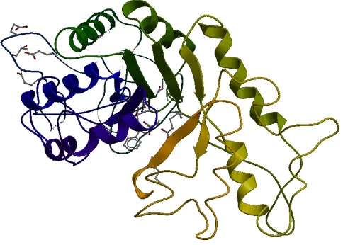
Figure 1.1: A non-obligate complex PDB ID 1avw with its interacting chains A and B, shown in different colors.

Figure 1.1 shows a non-obligate complex (PDB ID 1avw) an its two interacting chains

with different colors. This figure was generated with the help of ICM browser [48]. It

reflects how two chains of the protein complex interact with each other. The part of interest

is the interacting atoms. The complex is taken from one of datasets used in the proposed

model which is referred to as the Zhu dataset [50].

An important aspect in studying prediction of PPI is to predict different types of

com-plexes, including similarities between subunits (homo/hetero-oligomers), number of

sub-units involved in the interaction (dimers, trimers, etc.), duration of the interaction (transient

vs. permanent) [31], stability of the interaction (non-obligate vs. obligate) [50], among

others; but I focus on the problem of prediction protein interaction types (obligate and

non-obligate).

Obligate interactions are usually considered as permanent, while non-obligate

interac-tions can be either permanent or transient [33]. Non-obligate and transient interacinterac-tions are

(19)

and permanent interactions last for a longer period of time, and hence are more stable [22].

The study of [2] suggested that mobility differences of amino acids are more significant for

obligate and large interface complexes than for transient and medium-sized ones.

(a) Obligate complex PDB ID 1luc (b) Non-obligate complex PDB ID 1tab

Figure 1.2: Differentiating between Obligate and Non-obligate protein complexes on the basis of the interface area. Part (a) of the figure shows an obligate complex while the other part (b) depicts a non-obligate complex.

Figure 1.2 depicts an obligate complex (PDB ID 1luc) and a non-obligate complex

(PDB ID 1tab). It shows how obligate and non-obligate complexes differ from each other.

Observing part (a), the two chains of the complex are shown in different colors, i.e, yellow

and green. Since it is an obligate complex, it has larger interface area as compared to the

other complex. On the other hand, it is a non-obligate complex (PDB ID 1tab) with two

chains interacting with each other but with comparatively smaller interface area. Thus, on

the basis of the interface area one would be able to differentiate between the two types of

complexes. However, this is not the general case, since other properties may empower the

prediction, as shown in this thesis.

Non-covalent interactions are very common between macromolecules (including

(20)

i) Electrostatic interactions - they occur between electrically charged atoms having both

positive and negative interactions.

ii) Vander waal interactions - they occur between any pair of charged atoms that are close

to each other.

iii) Non-polar interactions - these are attractive interactions occurring between atoms that

do not have charges.

Two atoms that are either partially or fully electrostatically charged will interact with

each other. Each interacting atom generates an electric field that surrounds the atom. Also,

there are a few types of electrostatic interactions which are dominant in proteins :

i) Ionic interactions: they occur between fully charged atoms.

ii) Hydrogen bonds: they occur between atomic dipoles. They involve atoms with partial

charge, one of which is a hydrogen atom.

To predict the interaction types, every prediction method needs observed properties of

the known class samples called f eatures. Features are generally nominal or numeric, and

the process of calculating the features for each sample from the input dataset is called

fea-ture generation. Physiochemical properties of proteins are very powerful for prediction and

have been extensively reported in literature. Interacting regions can be characterized by

diverse sets of physiochemical properties [37], topological properties [10] and conserved

residues [27]. In addition, other properties have been used for PPI prediction such as

anal-ysis of solvent accessibility [50], geometry [25], hydrophobicity [44], sequence-based

fea-tures and desolvation energy [4],[44]. Based on interface properties such as interface area

and ratio of area [50], Zhuet al.predicted biological and crystal packing interactions using

(21)

properties, prediction of types (obligate and non-obligate) was reported using SVM and

linear dimensionality reduction (LDR) [43]. A very recent work presented by Ruedaet al.

shows the use of desolvation energies to solve the same prediction problem using the above

mentioned classifiers [30].

To reduce the size of the generated features from the input, feature extraction methods

have been used. Feature extraction is a popular pattern recognition method [18]. It is a

spe-cial form of dimensionality reduction. When the length of the feature vector is very large,

there might be a need to apply feature extraction methods to find the lower dimensional

representation of that original feature vector. The transformation of high dimensional data

to lower dimensional data is also called feature extraction [18]. There are many feature

ex-traction methods such as principal component analysis (PCA) [21], non-linear dimension

reduction, independent component analysis and linear dimensionality reduction (LDR). For

classification purpose, I use LDR methods [41] coupled with Bayesian classifiers (details

discussed in Chapter 3), which are the following:

• Fisher’s discriminant analysis (FDA) [12, 15].

• Heteroscedastic discriminant analysis (HDA) [28].

• Chernoff discriminant analysis (CDA) [41].

Lower dimensional data obtained by these three LDR methods are then passed through

quadratic Bayesian (QB) and linear Bayesian (LB) classifiers [12] for final prediction. For

each classifier, prediction accuracy and time taken for that prediction are very important. It

actually depends on the dataset used as well the behaviour of the classifier on a particular

(22)

1.2 Motivation and Objectives

Since PPI plays important role in many biological processes occurring in cells such as

cellular motion, gene regulation and transduction, many researchers are working to

un-derstand these different biological functions based on protein sequence or their structure.

Researchers are conducting their research work either by following labour intensive

experi-mental or computational approaches. Thus, understanding these biological functions, helps

understand diseases and develop drugs for their cure. Valuable knowledge generated by

these computational methods about these interactions greatly helps biological research.

During their life span, proteins interact with each other or even within themselves to

change their shape or other complexes to perform a specific biological function.

Previ-ously labour intensive approaches were available such as affinity chromatography or

co-immunoprecipitation. These days, high throughput methods such as tandem affinity

pu-rification, mass spectroscopy, yeast two hybrid, bimolecular fluorescence complementation

are available. But these methods are not applicable to all the proteins in all the organisms as

they suffer from some system errors [1, 16, 40]. Therefore, new computational approaches

are attracting more researchers for studying protein-protein interactions due to the fact that

these are cost effective. I propose a computational model, which I call PPIEE

(protein-protein interaction using electrostatic energy), to predict and analyze (protein-protein interaction

types (obligate and non-obligate) using electrostatic energies as properties. Thus, studying

these two types of PPIs will help researchers gather more information for understanding

and explaining biological processes and mechanisms for complex formation. It may also

help in drug development for curing diseases related to PPI.

Different features and prediction methods can be used to solve this specific problem. In

(23)

better than previously used properties such as NOXclass features (interface area, interface

area ratio, amino acid composition of the interface, correlation between amino acid

com-positions of interface and protein surface, gap volume index and conservation scores of the

interface) [50], desolvation energies [4], and others. With the proposed properties, I also

implement a model grouping by amino acids or by atom types for prediction purposes.

1.3 Problem Statement

In this thesis, I study the problem of predicting and analyzing protein-protein interaction

types (obligate and non-obligate) using electrostatic energies as properties. The aim is to

distinguish between two types of complexes, i.e. obligate and non-obligate, as mentioned

above. It is a very important problem in the field of proteomics.

1.4 Hypothesis

The thought for using electrostatic energies as properties in the proposed PPIEE is due to

the fact that electrostatic interactions are long ranged. These may go upto 10 ˚A or even

more. Thus, they cover wider interface area yielding more knowledge about atoms present

in the interface. There has been a lot of research in field of electrostatic energies. But the

idea of using these energies as properties to predict the protein interactions types (obligate

and non-obligate) is innovative and a framework has been designed to evaluate and validate

(24)

1.5 Contributions

I focus on prediction of two types of protein-protein interactions, namely obligate and

non-obligate to evaluate the results efficiently. The main contributions in this thesis are:

• To calculate the electrostatic energies for the Zhu dataset [50] and the Mintseris

dataset [32] using computer tools knowns as PDB2PQR [11] and APBS [5].

• To propose PPIEE that uses electrostatic energies as properties to predict

protein-protein interaction types.

• To integrate data from four different file formats, namely PDB, PQR, OUT and

IN-TERFACE.

• The use of electrostatic energies on these datasets with different grouping criteria

such as by atom types and amino acids.

• Visual analysis using electrostatic potential for some complexes in order to analyze

interactions from a different perspective.

In summary, I propose PPIEE to solve this type of problems efficiently and effectively.

The development of an automatic tool is important, which downloads the structural

infor-mation from PDB [7], and calculates the pairs of atoms in the interface for a particular

threshold distance and then, computes their electrostatic energies. Then, it arranges the

data in the form of features so that classification can be applied to predict the interaction

(25)

1.6 Thesis Organization

The thesis is organized in six chapters. Chapter II provides a survey of obligate and

non-obligate PPI and the prediction methods used to determine those types. Chapter III presents

different feature generation methods that can be used for prediction. Chapter IV describes

the proposed PPIEE model and features, and all required methods for the experiments.

Chapter V discusses the experimental results with the proposed approach and comparisons

with some of the existing methods. Finally, Chapter VI concludes the thesis with some

(26)

Chapter 2 Obligate and Non-obligate PPI

Prediction

2.1 Proteins

In 1838, Dutch chemist Gerhardus Johannes Mulder first described proteins, which were

named by Swedish chemist J ¨ons Jakob Berzelius [46]. Proteins are the most important

class of biochemical molecules, although lipids and carbohydrates are also essential for

life. Proteins are the basis for the major structural components of human and animal tissue.

Proteins are natural polymer molecules consisting of amino acids. The number of amino

acids in a protein may range from a few to several thousands. In general, a protein is an

organic compound, made of an arranged chain of amino acids which forms a globular or

fibrous form [46].

(27)

2.2 Protein Structures

A protein is a polymer of amino acids that has four levels of structure [38]:

1. Primary

2. Secondary

3. Tertiary

4. Quaternary

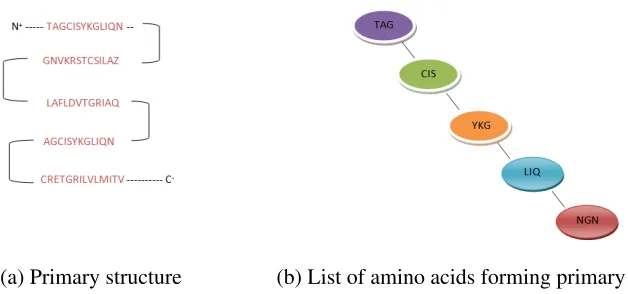
Figure 2.1 shows the primary structure of a typical protein which is made up of a

se-quence of amino acids along their backbone. Figure 2.1 (a) shows the linear sese-quence

of amino-acids that starts from amino terminal (N) end to the carboxyl-terminal (C) end.

Counting the residues always starting at the N terminal ((NH2)group), which is the place

in which the amino group is not involved in the peptide bond. The sequence of the protein

is unique to that protein and also defines its structure and function. Figure 2.1 (b) shows a

representation of primary structure of a portion of the protein in a different format. It shows

some of the 20 standard amino-acids such as alanine, proline, valine etc, in the three letter

code format. The structure is held together by peptide bonds which take place during the

(28)

CHAPTER 2. OBLIGATE AND NON-OBLIGATE PPI PREDICTION 13

(a) Primary structure (b) List of amino acids forming primary structure

Figure 2.1: Primary structure of a typical protein- a linear sequence of amino acids begin-ning from amino-terminal N to carboxyl-terminal C.

The secondary structure as shown in Figure 2.2 consists alpha helices, beta sheets and

turns. These were suggested in 1951 by Linus Pauling and are defined by patterns of

hy-drogen bonds among the main chain peptide groups.

(a) Alpha helix (b) Beta sheet

(29)

Figure 2.2(a) represents an alpha helix in which it is coiled like a loosely coiled spring.

The coiling occurs in clockwise direction as it goes away from us. The main criteria for

the alpha helix is that the amino acid side chain should cover and protect the backbone

(H-bonds). Attractive forces between different atoms cause formation of specific structures.

Figure 2.2(b) shows beta-pleated sheets in which chains are folded so that they lie along

with each other. These sheets are actually anti-parallel in nature. The folded chains are

held together by hydrogen bonds that makes them more stable in nature. The figures were

generated with the help of ICM browser [48] by entering complex PDB ID 1ava, which is

obtained from the Zhu dataset [50].

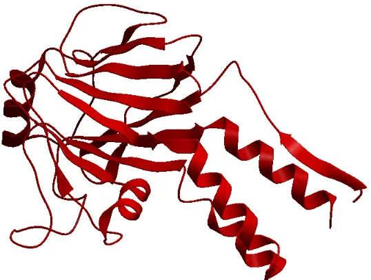
Tertiary structure is the three-dimensional structure of a single protein molecule. The

alpha helices and beta sheets are folded into globular form. This folding is mainly due to

the hydrophobic interactions. Figure 2.3 shows the tertiary structure of PDB ID 1dev, chain

A. It is a combination of alpha helices as ribbons and beta sheets as arrow heads. It is

made up of several domains and each domain has its own function. The bits of the protein

chain which are just random coils or loops are shown as bits of strings. These structures are

diverse and more complex and largely determined by the biomolecule’s primary structure

or the sequence of amino acids. Its amino acids are capable of performing diverse functions

ranging from molecular recognition to catalysis. The figure was generated with the help of

(30)

Figure 2.3: Tertiary structure as one sub-unit of PDB ID of 1dev (Chain A), a non-obligate complex. The structure is a combination of alpha helices shown as ribbons and beta sheets shown as arrow heads.

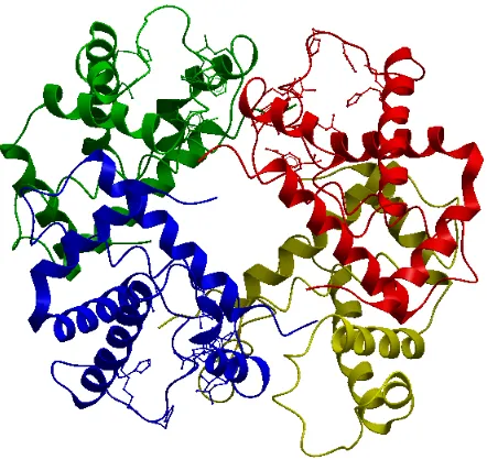
Quaternary structure is the arrangement of multiple folded proteins in a multi-subunit

complex. The quaternary structure of a protein can be determined by experimental

tech-niques by placing a sample protein in different experimental positions. Most of the proteins

in the human body are found in this state. Examples of proteins in that state include DNA

polymerase, hemoglobin and ion channels.

Figure 2.4 shows an example of a protein in its quaternary structure. The four different

colors represents four different chains for 1a3n, i.e., Chains A, B, C and D. These sub-units

yield a stable structure. This structure involves the clustering of several individual protein

chains into a specific shape. PDB ID 1a3n (hemoglobin) is a type of Globular quaternary

protein which is clumped into a ball shape as shown. Other examples are insulin and most

of the enzymes. This structure may fall apart in a high salt environment. This figure was

(31)

Figure 2.4: Quaternary structure of PDB ID 1a3n, hemoglobin, consisting of Chains A, B, C and D respectively. The four different chains are represented in different colors for clarity.

2.3 Protein-protein Interactions

To perform biological functions, one or more proteins may bind to each other or to DNA

or RNA. This is the main reason why protein interaction takes place inside human body.

Protein-protein interaction involves [33]:

• Direct contact association of molecules, which means that different molecules

be-longing to specific amino acids within a protein may interact with each other if they

are close to each other under a certain threshold distance. Generally, for direct

asso-ciation molecules, they should be within 7 ˚A distance from each other [8].

• However, if I consider the role of electrostatic interactions, these are considered to be

(32)

take place, if the molecules are within the distances of 10 ˚A or even more [23].

Figure 2.5: Protein-protein interaction for complex PDB ID 1cli. The highlighted area indicates the interface or the place where interaction occurs between the two chains.

Figure 2.5 shows two interacting chains, Chains A and B of PDB ID 1cli. The

inter-acting chains are shown in green and red respectively. The highlighted portion shows the

interface where the actual interaction takes place. This figure gives a clear idea how two

chains interact with each other, forming a complex. This region is the area of interest,

since electrostatic energies for the pairs of atoms present in this region are calculated using

available software packages. This figure was generated using ICM browser [48].

There is a need to understand how proteins interact with each other. Since proteins

per-form different biological processes in a cell including cell growth, nutrient uptake, motility,

intercellular communication and apoptosis. Critical aspects required to understand

func-tions of proteins include [17]:

• Protein sequence and structure- used to discover motifs that predict protein func-tion.

(33)

• Interactions with other proteins- functions may be predicted by knowing the func-tion of binding partners.

• Post translational modifications - even some changes after the interaction take place.

2.3.1 Domains

The concept of domains was first proposed in 1973 by Wetlaufer [29]. A domain is a three

dimensional structure that is part of a protein. It evolves, functions and exists independently

from the rest of the protein chain. Domains may vary in length from 25 to 5,000 amino

acids. Physical interaction between proteins is also analysed on the basis of the residues of

their structural domains. The presence of multiple domains gives rise to great flexibility and

mobility. As a result, domain-domain interactions, these properties can be used to predict

protein-protein interaction types [29].

Figure 2.6: Representation of domains in complex PDB ID 1ava (chain A).

(34)

domains were discovered using the Pfam server [39], which represent protein families or

domains. The server helps in determining the domains and it carries its architecture. The

residues belonging to Chain A beginning from 17 and ending at 324 were found to be a

domain and is shown in the figure. This figure was generated using ICM browser [48].

2.3.2 Motifs

A motif refers to a particular amino acid sequence that is characteristic of a particular

bio-logical function. An example is the zinc finger motif, which is a functional motif. In other

words, it is a set of contiguous secondary structure elements that has specific functional

significance or defines a portion of an independently folded domain. Identifying motifs

from a sequence is not straightforward since they have functional implications. Some

mo-tifs such as the zinc finger motif are easy to identify since they are continuous but other

might be discontinuous and might be then difficult to predict. Short linear motifs are short

stretches (also known as SLiMs or minimotifs) of a protein sequence that help mediate

protein-protein interaction. The main role of SLiMs is to target specific interactions with

other protein domains [9].

The sequence logo is a useful graphical representation of the protein motifs. It shows

how well amino acids are conserved at each position; the higher the frequency of amino

acids, the higher the letter will be, because the better the conservation is at that position.

Different amino acids at the same position are scaled according to the information content

of that amino acid.

Figure 2.7 shows the sequence logo for the short, linear motif found on the chains of

Cytoplasmic Malate Dehydrogenase (PDB ID 4mdh) complex at position 233. The Regular

(35)

-axis which represents the positions of the SLiM, and they-axis that reflects the information

content of that specific position. The information content of they-axis is given by (2.1):

Figure 2.7: One short, linear motif found in both chains of Cytoplasmic Malate De-hydrogenase (PDB ID 4mdh) at position 233. The regular expression of this SLiM is [RN][YDG]I[GRW][YF]G.

Ri=log2(20)−(Hi+en). (2.1)

whereHiis the uncertainty of a positioniandHiis defined as:

Hi=−

∑

fa,i log2 fa,i. (2.2)

Here, fa,iis the relative frequency of amino acidaat positioni, enis the small-sample

correction for an alignment ofnletters. The height of letterain columniis given by (2.3):

en=

(s−1)

(36)

For proteins, the value ofsis 20 andnthe length of the SLiM.

2.3.3 Protein-protein Interaction types

Another important aspect in studying PPI is to predict different types of complexes,

includ-ing similarities between subunits (homo/hetero-oligomers), number of subunits involved in

the interaction (dimers, trimers, etc.), duration of the interaction (transient vs. permanent)

[31], stability of the interaction (non-obligate vs. obligate) [50]. Based on physiological

functions, specificity and evolution, PPIs can be divided into four broad categories [33]:

1. Homo and hetero-oligomeric interactions

2. Non-obligate and obligate interactions

3. Transient and permanent interactions

4. Crystal packing and biological interactions

Homo-oligomer and hetero-oligomeric interactions: If the two interacting protein chains of an oligomer have structural symmetry, then those kinds of PPIs are called

homo-oligomeric protein-protein interactions. If the two interacting protein chains of an oligomer

have differences in their structure, those kinds of PPIs are called hetero-oligomeric

(37)

Figure 2.8: Homo-oligomer complex PDB ID 2gbl.

(38)

Figure 2.8 depicts the quaternary structure of PDB ID 2gbl which is a homo-oligomer

complex. This complex contains six identical units, all reflected in different colors which

are structurally similar to each other.

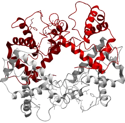
Figure 2.9 shows another complex, PBD ID 1a3n, Hemoglobin. It is made up of two

homo-dimers as shown in different colors, red and white.

Obligate and Non-obligate interactions: Obligate interactions are usually considered as permanent, while non-obligate interactions can be either permanent or transient [33].

Non-obligate and transient interactions are more difficult to study and to understand due to

their instability and short life, while obligate and permanent interactions last for a longer

period of time, and hence are more stable [22].

Transient and permanent protein-protein interactions: These kinds of interactions are differentiated on the basis of the lifetime of the interacting protein complexes.

Perma-nent interactions are stable interactions, while transient interactions are less stable

interac-tions.

Crystal packing and biological interactions: During the process of crystallization protein complexes form solid crystals [50]. These kinds of interactions do not serve the

biological purpose because they are incapable of performing any biological activity. This

type of packing is called crystal packing interaction. All other PPIs that occur perform

some biological functions and are called biological PPI.

PPIs can take place between identical or non-identical chains which are based on their

structural similarity. If the interacting chains of an oligomer has structural symmetry, then

it is called homo-oligomeric PPI, otherwise it is called hetero-oligomeric PPI. While

con-sidering the life time of a complex, it can be a transient and permanent PPI. Permanent PPIs

(39)

chang-ing their shapes until they dissociate or result in permanent complexes. To find out about

the biological functions performed by different types of complexes, it is important to know

about the PPIs.

2.4 Protein-protein Interaction Prediction Approaches

Many researchers worked on predicting protein-protein interaction types with different

ap-proaches. These approaches are mainly divided into two main categories, namely:

1. Experimental Approaches

2. Computational Approaches

Traditionally, prediction of PPI was limited to experimental techniques such as

co-immunoprecipitation or affinity chromatography [1, 16, 40]. These methods are

labor-intensive and often the results of these approaches contain systematic errors. Since the data

for prediction is growing, these experimental processes become less applicable.

Compu-tational approaches are more popular these days because they are less expensive to use.

Computational approaches can be further divided into two classes.

1. Methods based on evolutionary conservation information

2. Those solely structure based on geometrical and physiochemical properties of the

proteins.

Modern multiple sequence alignment algorithms including residue substitution

matri-ces allow detection of conservation signal. One type of prediction depends on the algorithm

for deriving scores from the alignment [34]. But the main problem is that many protein

(40)

assumption that protein interfaces are quite different from the rest of the surface, since they

vary in their geometrical and physiochemical properties from rest of the surface. The

phys-ical properties of the interface are highly diverse [36]. To decide between which approach

is better depends upon the nature of the protein of interest and available resources.

To predict obligate and non-obligate PPIs, many classifiers including random forest (RF),

Bayes, decision trees, logistic regression, neural networks, SVM and LDR have been used.

Different classifiers achieve different performances based on the type of data and

prop-erties used. Some research in [12, 15, 41] achieved a classification accuracy of 70% for

the problem of distinguishing obligate and non-obligate interactions with a wide range of

parameters and different types of features such as desolvation energy, amino acid

composi-tion, conservation scores, electrostatic energies, and hydrophobicity.

Descriptors based on the 3D structure of proteins used for the prediction are as follows

[24]:

1. Neighbour list: Residues in the spacial vicinity to the residue in question. Generally, 9-20 residues are taken into consideration.

2. β Factor: It is the crystallographic measure that approximates the flexibility of the residue.

3. Secondary structure: This structure represents alpha helices, beta sheets and loops. 4. Sequence distance: The separation between residues within the same patch. Some results shows that structurally contiguous residues are more likely to form interaction

sites.

(41)

1. Sequence profile: Extracted from multiple sequence alignment, profiles reveal pat-terns of evolutionary conservation.

2. Conservation Score: A quantification of the level of conservation of an individual position.

3. Conservation of physiochemical traits: If the position is not conserved, scoring conservation of traits such as charge, hydrophobicity, or size may improve prediction.

Descriptors based on physiochemical properties:

1. Hydrophobicity: It is the physical property of a molecule that is repelled from mass of water. Hydrophobic molecules often cluster together in water to form micelles.

Several different scales are available.

2. Electrostatic potential: It co-relates with the dipole moment, electro-negativity and partial charges. In other words, it is the potential energy of the protons at a particular

location near a molecule. It requires the 3D structure of the protein.

3. Atom propensities: It serves as a way to sum physiochemical properties across residues in a patch.

4. Desolvation energies: Used in prediction of protein interaction types and rigid-body docking.

The proposed PPIEE model uses LDR and SVM methods for classification. PPIEE uses

LDR coupled with Bayesian both linear and quadratic. The details of these classifiers are

(42)

Chapter 3 Feature Extraction and Prediction

3.1 Pattern Recognition

Pattern recognition is the scientific field whose goal is clustering, feature selection and

extraction and classification of objects into a number of categories or classes [45]. An

example of pattern recognition is classification whose aim is to assign labels to unknown

objects. A simple example can be whether to determine that a given email is spam or

non-spam. Generally speaking, the objects can be protein sequences, signal waveforms or

images. There are several application areas of pattern recognition in today’s world. It is the

most important part for the machine learning systems built for decision making. Typical

applications are automatic speech recognition, classification of text in several categories

and automatic recognition of images of human faces.

In machine learning and pattern recognition, one of the key factors is to include and

select the right features for successful prediction. These are the observed properties of each

sample that are used for prediction. The value of the features are usually numeric, but other

types such as strings and graphs are also used.

(43)

3.1.1 Classifiers

In pattern recognition, classification is the procedure for identifying unknown samples on

the basis of training sets of known samples. The classification problem is known as

super-vised learning in pattern recognition. In supersuper-vised learning, the training set is provided

with labels attached to each sample. Then, the classifier is trained on these samples. After

the classifier is well trained, it can classify unknown samples. On the other hand,

unsu-pervised learning assumes that training data do not have labels attached to the samples and

attempts to find the inherent patterns in the data that can hopefully determine the correct

output value for new unknown instances. There are various classifiers available [14]:

1. Linear classifiers

2. Quadratic classifiers

3. Support vector machine

4. Decision tree

5. Neural Networks

6. Hidden Markov Models

Among these, I use SVM, linear classifiers and quadratic classifiers for prediction of

obligate and non-obligate types of interactions.

3.2 Features Used for PPI Prediction

(44)

CHAPTER 3. FEATURE EXTRACTION AND PREDICTION 29

β-factor : It is the flexibility of the protein complexes during the interaction.

Solvent Accessibility : It is the exposed surface area that affects contact of atoms during the interaction.

Geometric features : The shape index, planarity or curvedness of the interacting com-plexes can also be used as features.

Evolutionary features : They include conservation scores or sequence profiling informa-tion.

Physicochemical features : They include hydrophobicity, electrostatic and desolvation energies.

3.2.1 Tools Used to Calculate Electrostatic Energies

Electrostatic interactions are important in understanding intermolecular interactions. These

interactions control the structure and binding of biomolecules. Electrostatics are important,

since they are long ranged interactions and because of their influence in charged molecules

[5]. This motivated me to focus on electrostatic energies and hence use them as properties

for predicting interaction types.

In order to compute electrostatic energies, software packages including PDB2PQR [11]

and APBS [6] were used. PDB2PQR was written by Todd Dolinsky while working with

Nathan Baker at Washington University in St. Louis, USA. PDB2PQR is a tool that

auto-mates common tasks for preparing structures for electrostatic calculations. Its purpose is

to add missing heavy atoms, place missing hydrogen atoms and assign charge and radii to

PDB files. The output of this package is a PQR structure file, which is the input for APBS.

(45)

the software can be run with customized parameters. The command line argument which

executes the Python script is in (3.1).

$ python pdb2pqr.py [options] –ff={forcefield} {path} {output path} (3.1)

This software provides many parameters which can be customized as per needs which

are as follows:

• forcefield: Currently this software supports AMBER, CHARMM, PARSE and TYL06 forcefields.

• path: It requires the input path to the PDB complex. The software will execute this PDB file to output PQR file format.

• output-path: It requires the desired name of the PQR file. The file will be saved on the path or location specified here in this parameter.

• chain name(optional): It keeps the chain ID in the output of the PQR file format. • –asign-only(optional): It only assigns charge and radii. It does not add atoms, or

debump, or optimize.

• –noopt(optional): It does not perform hydrogen bonding network optimization. • –apbs-input(optional): It creates the template APBS input file based on the

gener-ated PQR file. It further has some parameters that can be changed to run APBS.

(46)

APBS is a software package used for calculating electrostatic energies for interactions

between solutes in salty and aqueous media [6]. It solves the Poisson-Boltzmann equation

numerically and evaluates electrostatic calculations ranging from tens to millions of atoms.

It basically uses Fekt (Finite element toolkit) which solves the Poison-Boltzmann

equa-tion for electrostatic calculaequa-tions. It is used for modelling bio-molecular solvaequa-tion through

solution. This software was written by Nathan Baker in collaboration with J.Andrew

Mc-Cammon and Michael Holst. APBS is also integrated with other programs such as Jmol,

which help visualize the complexes for better understanding.

APBS can be run either through the web-server or it can be installed on a local machine.

The advantage of installing it and running it on a local machine is that it provides the

freedom to use more parameters. For PPIEE, electrostatic energies per atom were calculated

using APBS. The command line used to run APBS is in (3.2).

f or i in∗.in; do

echo ”Running $i...”

(apbs $i2>&1)∥tee ${i%.in}.out

done

(3.2)

Some of the parameters which need to be taken care of while running APBS are in the

elecsection as follows:

• Calcenergy: Changing the parameter Calcenergy “total” to Calcenergy “comps”. The software produces the electrostatic energies per atom.

(47)

3.3 Proposed Features on Electrostatic Energies

I consider the interaction between theithatom of the first interacting chain and the jthatom

of the second interacting chain. Then, I calculate the distance between all possible atom

pairs. If an atom pair is separated by a distance less than or equal to a certain threshold,

that pair is considered to be in the interface of that complex [23]. In most studies,

inter-atom distances are not greater than 7 ˚A. But in order to achieve an in-depth analysis for

electrostatic energies as properties, in this work, the threshold was varied from 7 ˚A to 13 ˚A.

It is to be noticed that even the atoms that are under the surface of proteins pose electrostatic

forces towards the stability of the protein complex.

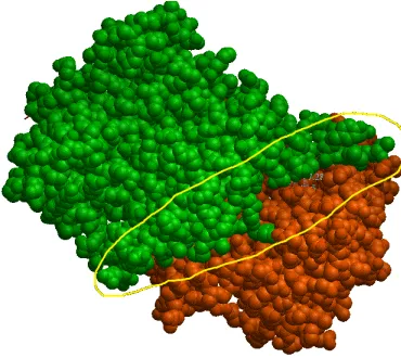
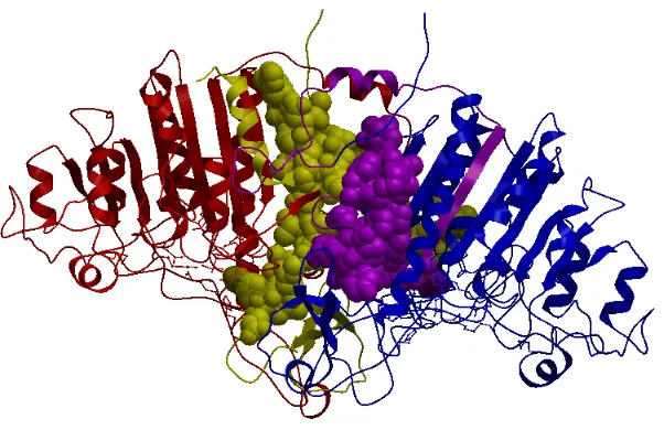
Figure 3.1: An obligate complex PDB ID 1b8j with its interacting chains A and B as shown in different colors, red and blue. This figure was generated with the help of ICM browser. [48].

Figure 3.1 depicts an obligate complex, PDB ID 1b8j, along with its interacting chains

(48)

of distance act as interface atoms and are represented as yellow and purple spheres

respec-tively. An atom pair is considered to be in the interface if atoms are under certain threshold

distance apart from each other for this complex. Since electrostatic interactions are long

ranged, a larger interface area is observed.

3.4 Feature Generation

For each complex in the datasets, structural data from PDB [7] were collected. Two

inter-acting chains were extracted from each PDB file. I consider 18 different atom types as in

[49]. Thus, for each protein complex a feature vector with18C2+18 = 171 values were

ob-tained, where each feature contains the cumulative average of electrostatic energies for all

pairs of atom of the same type in the interface. Since the order of interacting atoms in the

pairs is not important, the final length of the feature vector for each complex is 171 which

corresponds to the number of unique pairs [42]. I have also considered pairs of amino acids,

and for this, I computed20C2+20 = 210 values for all pairs of amino acids and by

accumu-lating the electrostatic values of the corresponding atoms for each pair of amino acids. The

final length of the feature vector for each complex is 210 which corresponds to the number

of unique pairs for 20 standard amino acids. This is how I obtain feature vectors for both

atom types (171) and amino acid types (210). Averages for electrostatic values for the pairs

of atom types and amino acids are calculated as follows:

Σ(ei+ej)/2. (3.3)

whereeistands for the electrostatic value for theithinterface atom from the first interacting

(49)

interacting chain.

Using Equation (3.3), for each complex in the datasets, the averages of electrostatic

values were computed for the pairs of atoms on the interface. There are 18 unique type of

atoms and 20 amino acids. Table 3.1 [49] is an 18×18 matrix, where all possible

combi-nations of 18 unique atom types are represented. If the interacting chains of a complex are

known, the very first task is to find the interacting atoms from both chains under a certain

threshold value. Then, the conversion for all the interface atoms to their corresponding

unique types is done. The method of conversion is derived from the conversion table that is

discussed in [49]. Based on PPIEE experiments and the study of [49], Tables 3.2 and 3.3 are

used for atom type conversion. In these conversion tables, the first row of each amino acid

contains the original atoms that are inside them and the second row contains the converted

unique atom-types. When the unique types are determined, I simply find that pair in the

table and obtain the unique types for the atoms. In order to find the interface atoms, I find

the Euclidian distance between the two atoms from two interacting chains, which is to be

computed from their structural data that can be found in PDB files [7].

Table 3.1 shows an example for the atom-type table. The averaged electrostatic values

for the pairs of atoms are stored in their respective positions as shown in the table. With the

help of Table 3.2 [49], I was able to determine a unique type for every atom in the interface.

Just as an example, if I know that atom Nitrogen belongs to amino acid Alanine, then its

(50)

3.4.1 Classifiers Used in This Work

3.4.1.1 Bayesian Decision Theory

Bayesian decision theory is a fundamental statistical approach for pattern classification. It

assumes that decision problems are based on probabilistic terms. The main focus of this

work is about the discriminant function for normal densities. The expression for the

multi-variate normal distribution is [13]:

gi(x) =−1₂(x−µµµi)t ∑−i 1(x−µµµi)−d2 ln 2π− 1

2 ln|∑i|d+ ln P(ωi). (3.4)

wherex is a d−component column vector, µµµ is a d− component mean vector and Σ is thed × d covariance matrix, which is always symmetric and positive semidefinite, and

P(ωi)are the prior probabilities.

Some special cases for the discriminant functions are the following:

Case 1: This case is when the features are statistically independent and have the same

variance, σ2. Geometrically, this case is when samples fall on equal-sized clusters. The

discriminant function is:

gi(x) =−_2σ12[xtx−2µµµti x+µµµtiµµµi] + ln P(ωi). (3.5)

Case 2: When the covariance matrices for all the classes are identical but otherwise

arbitrary. Geometrically, in this situation all the samples fall on hyper ellipsoidal clusters

(51)

gi(x) =−1₂(x−µµµi)t Σ−1(x−µµµi) + ln P(ωi). (3.6)

where for two classesΣican be obtained as:

Σ= 1₂[Σ1 + Σ2]. (3.7)

In (3.6)P(ωi)is the prior probability of classωi. To classify each feature vectorx, one

measures the squared Mahalanobis distance from eachxto each of thecmean vectors and assignxto the category of the nearest mean.

Case 3: It is the general multivariate normal case, in which the covariance matrices are

different for each category. This is called quadratic Bayesian classifier (QB). The

classifi-cation function is as follows [13]:

gi(x) = xtWix+wt_i x+ωi0. (3.8)

whereWiis:

(52)

andwiis:

wi=∑−i 1µµµi. (3.10)

3.4.1.2 Linear Dimensionality Reduction

The basic idea of LDR is to represent an object of dimensionn (171 or 210) as a

lower-dimensional vector of dimension d, achieving this by performing a linear transformation.

Consider two classes, obligate asω1and non-obligate as ω2, represented by two normally

distributed random vectorsx1∼N(m1,S1)andx2∼N(m2,S2), respectively, with p1 and

p2thea prioriprobabilities. After the LDR is applied, two new random vectorsy1=Ax1

andy2=Ax2, wherey1∼N(Am1; AS1At)andy2∼N(Am2; AS2At)withmiandSi

be-ing the mean vectors and covariance matrices in the original space, respectively. The aim of

LDR is to find a linear transformation matrixAin such a way that the new classes (yi=Axi)

are as separable as possible. LetSW =p1S1+p2S2andSE = (m1−m2)(m1−m2)t be the

within-class and between-class scatter matrices respectively. Various criteria have been

proposed to measure separability between the classes [41]. I focus on the following three

LDR methods:

Fisher’s discriminant analysis (FDA) [12, 15] : Its optimization criterion is as follows:

JFDA(A) =tr

{

(ASWAt)−1(ASEAt)

}

(3.11)

(53)

eigenvalue ofSFDA=S−_W1SE.

Heteroscedastic discriminant analysis (HDA) [28] : It aims to obtain the matrixA that maximizes the function:

JHDA(A) =tr

{

(ASWAt)−1[ASEAt −AS

1 2

W p1log(S

−1 2

W S1S

−1 2

W )+p2log(S

−1 2

W S2S

−1 2

W )

p1p2 S

1 2

WAt

]}

(3.12)

This criterion is maximized by obtaining the eigenvectors, corresponding to the largest

eigenvalues, of the matrix:

SHDA=S_W−1

[

SE−S

1 2

W p1log(S

−1 2

W S1S

−1 2

W )+p2log(S

−1 2

W S2S

−1 2

W )

p1p2 S

1 2

W

]

(3.13)

Chernoff discriminant analysis (CDA) [41] : It aims to maximize the following func-tion:

JCDA(A) =tr{p1p2ASEAt(ASWAt)−1

+log(ASWAt)−p1log(AS1At)−p2log(AS2At)}

(3.14)

In this work I use the gradient-based algorithm proposed in [41], which maximizes the

function in an iterative way. For this gradient algorithm, a learning rate, αk needs to be

computed. In order to ensure that the gradient algorithm converges, αk is maximized by

using the secant method. One of the keys in this algorithm is the random initialization of

(54)

3.4.2 Support Vector Machine

I also use SVM, which is widely used in bioinformatics for classification. It takes the set of

input vectors and predicts the possible classes of output based on the support vectors [19].

The kernel trick allows one to map the original vectors onto a much higher dimensional

space that hopefully makes class separation easier. Basically, there are two kinds of

mar-gins in SVM. The first one is called hard margin and the second one is called soft margin.

In the hard margin SVM, the training data is linearly separable in the input space while in

soft margin data can be either be linearly or non-linearly separable. If the training data is

not linearly separable they can be mapped onto a higher dimension feature space to increase

separability.

3.4.2.1 Hard-Margin Support Vector Machine

LetXi(i = 1, ....n)bed-dimensional training input vectors which belong to class 1 or class

2 and the corresponding labels beyi = 1 for class 1 andyi = −1 for class 2. For linearly

separable data the the decision function is as follows [3]:

(55)

Figure 3.2: Optimal separating hyperplane in the two dimensional space.

Figure 3.2 shows the optimal hyperplane which best classifies between two classes. As

shown in the figure, the hyperplane in blue has the maximum margin with respect to both

classes and is the calledoptimal separating plane.

The optimal separating hyperplane can be obtained by minimizing :

Q(w) = 1/2∥w∥2

with respect towandbsubject to the constraints:

yi(wTxi+b)>=1 fori = 1, ....M

The square of the Euclidean norm∥w∥is to make the optimization problem solvable by quadratic programming. The data is linearly separable, if there existswand bthat satisfy the above equation. In order to map the input vectors to a higher dimensional feature

space, with infinite dimensions, the above mentioned constraints are converted into the

unconstrained problem [3]:

Q(w,b,α) =1₂WTw− ∑n

i=1α

i[yi(wT)xi+b)−1]. (3.15)

whereα = α1, ....αmare the non-negative Lagrange multipliers. Then, the

(56)

Q(α) =∑m_i₌₁αi − 1₂∑Mi,j=1αiαjyiyjxTi xj. (3.16)

with respect toaisubject to the constraints:

∑M

i=1yiαi = 0 (3.17)

whereαi≥0 fori=1, ...M

All data associated withaiare known as support vectors and from the standard point of

precision of calculations, the average is calculated among the support vectors which is:

b = _∥1_S_∥∑_i_∈_S(yi−wTxi) (3.18)

Now the unknown datumxcan be classified into:

Class1i f D(x) > 0,

Class2i f D(x) <0

(3.19)

This function classifies the data into two different classes. In special case D(x) = 0, the sample is said to be unclassifiable.

3.4.2.2 Soft-Margin Support Vector Machines

Soft margin can also be used for the linearly separable data. But in case the data are

(57)

that aims to maximize the distance between the classes. Thus, following criteria is used [3]:

Q(w,b,β) =1₂ ∥w∥2+C∑M_i₌₁β_ip. (3.20) whereChas to be optimized.

3.4.2.3 The Kernel Trick

In SVM, the aim of the hyperplane is to maximize the separation between classes. But if

the training data are not linearly separable then the optimal hyperplane is not good enough.

Thus, to increase the separability, the original input vectors are mapped onto a higher

di-mensional dot product space called f eature space. For this, there is a mapping function

ϕ(x)that maps thexinto the dot-product feature space andg(x)satisfies [3]:

H(x,x′) = ϕt(x)ϕ(x′) (3.21)

Using the kernel trick, the problem in the feature space is as follows:

Q(a) = ∑M i=1α

i − 1₂ M

∑

i,j=1α

iαjyiyjH(xi,xj) (3.22)

and the problem is solved without explicitly mapping onto the feature space provided

that the kernel satisfies Mercer’s condition in (3.23). This whole procedure is calledkernel trick.

∑M

i,j=1hihjH(xi,xj) ≥0 (3.23)

Some kernels which are used in the SVM are as follows:

(58)

If a classification problem is linearly separable, then there is no need to map the data

onto higher dimensions. Thus, the linear kernel is as follows:

H(x,x′) = xtx′ (3.24)

• Polynomial kernel:

The polynomial kernel with degreed, wheredis a natural number, is given by:

H(x,x′) = (xtx′+1)d (3.25) Here one is added with degree equal to less thandare included.

• Radial Basis Function (RBF) kernels:

The RBF kernel is given by:

H(x,x′) = exp(−γ∥x−x′∥2 (3.26) whereγis a positive parameter for controlling the radius, which has to be optimized.

3.4.3 Prediction Evaluation

Cross validation plays an important role in validating prediction results. It is a technique for

assessing how the results of statistical analysis will generalize to unknown samples of any

dataset. It involves partitioning of sample data into subsets. The most common approach

used is theK fold cross validation. PPIEE uses 10-fold cross validation in classification.

Cross validation provides a framework for creating several train/test sets assuring that each

A model to predict and analyze protein-protein interaction types using electrostatic energies

Scholarship at UWindsor

Scholarship at UWindsor

A model to predict and analyze protein-protein interaction types

A model to predict and analyze protein-protein interaction types

using electrostatic energies

using electrostatic energies

A MODEL TO PREDICT AND ANALYZE PROTEIN-PROTEIN

INTERACTION TYPES USING ELECTROSTATIC ENERGIES

APPROVED BY:

Declaration of Co-Authorship

Dedication

Contents

List of Tables

Chapter 1

Introduction

1.1

Protein-protein Interaction

1.2

Motivation and Objectives

1.3

Problem Statement

1.4

Hypothesis

1.5

Contributions

1.6

Thesis Organization

Chapter 2

Obligate and Non-obligate PPI

Prediction

2.1

Proteins

2.2

Protein Structures

2.3

Protein-protein Interactions

2.3.1

Domains

2.3.2

Motifs

∑

2.3.3

Protein-protein Interaction types

2.4

Protein-protein Interaction Prediction Approaches

Chapter 3

Feature Extraction and Prediction

3.1

Pattern Recognition

3.1.1

Classifiers

3.2

Features Used for PPI Prediction

3.2.1

Tools Used to Calculate Electrostatic Energies

3.3

Proposed Features on Electrostatic Energies

3.4

Feature Generation

3.4.1

Classifiers Used in This Work

3.4.2

Support Vector Machine

3.4.3

Prediction Evaluation