ABSTRACT
SHAHIN, MAHDIZADEHAGHDAM. Exploiting Structure in Data: Depth and Dynamics. (Under the direction of Hamid Krim.)
Every aspect of human life can be monitored. Data can be gathered from health monitoring apps, images and videos in social networks, or even from personal aspects of our lives such as
financial and banking data. Due to the complex interactions within the data, inference from these
irregular structures, demands exploration of novel methods. The goal of this dissertation is to exploit structures in data and extract insights and knowledge from the massive amount of data available
around us. At the first attempt, we explore dynamics of spreading ideas in social networks. Next we
develop techniques to overcome the deficiencies of deep learning in analyzing high-dimensional data such as images.
Real-world social and/or operational networks consist of agents with associated states, whose connectivity forms complex topologies. This complexity is further compounded by interconnected information layers, consisting, for instance, documents/resources of the agents which mutually share topical similarities. We propose a method to predict the specific states of the agents, as their
observed resources evolve in time and get updated. The information diffusion among the agents and the publications themselves effectively result in a dynamic process which we capture by an
interconnected system of networks (i.e. layered). More specifically, we use a notion of a
supra-Laplacian matrix to address such a generalized diffusion of an interconnected network starting with the classical "graph Laplacian." The auxiliary and external input update is modeled by a
multidimensional Brownian process, yielding two contributions to the variations in the states of
the agents: one that is due to the intrinsic interactions in the network system, and the other due to the external inputs or innovations. A variation on this theme, a priori knowledge of a fraction of the
agents’ states is shown to lead to a Kalman predictor problem. This helps us refine the predicted
states exploiting the estimation error in the agents’ states.
Three real-world datasets are used to evaluate and validate the information diffusion process
in this novel layered network approach. Our results demonstrate a lower prediction error when
using the interconnected network rather than the single connectivity layer between the agents. The prediction error is further improved by using the estimated diffusion connection and by applying
the Kalman approach with partial observations.
We next propose a new framework based on deep dictionary learning to classify image. Deep
dictionary learning seeks multiple dictionaries at different image scales to capture complementary
coherent characteristics. We propose a method for learning a hierarchy of synthesis dictionaries with an image classification goal. The dictionaries and classification parameters are trained by a
classification objective, and the sparse features are extracted by reducing a reconstruction loss
hierarchical method increases by adding more layers, which consequently makes this model easier
to tune and adapt. The proposed algorithm furthermore, shows remarkably lower fooling rate in presence of adversarial perturbation. The validation of the proposed approach is based on its
classification performance using four benchmark datasets and is compared to CNNs of similar size.
Finally, we enhance the Generative Adversarial Networks (GANs), for image generation, by dividing an image into multiple patches and modifying the role of the generative network from
producing an entire image, at once, to creating a sparse representation vector for each image patch.
We obtain the entire image by multiplying sparse representations to a pre-trained dictionary and assembling the resulting patches. This approach restricts the output of the generator to a particular
structure, obtained by imposing a Union of Subspaces (UoS) model to the original data, leading to
more realistic images, while maintaining the desired diversity. To further assist GANs in generating high-quality images and to avoid the notorious mode-collapse problem, we introduce a third player
in GANs, called reconstructor. This player utilizes an auto-encoding scheme to ensure that first,
the input-output relation in the generator is injective and second each real image corresponds to some input noise. We present a number of experiments, where the proposed algorithm shows a
© Copyright 2019 by Mahdizadehaghdam Shahin
Exploiting Structure in Data: Depth and Dynamics
by
Mahdizadehaghdam Shahin
A dissertation submitted to the Graduate Faculty of North Carolina State University
in partial fulfillment of the requirements for the Degree of
Doctor of Philosophy
Computer Engineering
Raleigh, North Carolina
2019
APPROVED BY:
Tianfu Wu Huaiyu Dai
Wenbin Lu Liyi Dai
External Member
Hamid Krim
BIOGRAPHY
Shahin Mahdizadehaghdam received his M.S. degree in communication and computer networks from Sharif University of Technology, Iran, in October 2011. In August 2013, he started his PhD
in the Department of Electrical and Computer Engineering in North Carolina State University
and joined Vision, Information and Statistical Signal Theories and Applications (VISSTA) group under the direction of Dr. Hamid Krim. His research interests include dimension reduction, online
social network analysis, and machine learning. More specifically, he is interested in dimensionality reduction, sparse representations, and developing hierarchical dictionary learning methods for
ACKNOWLEDGEMENTS
First and foremost I express my special gratitude and thanks to my advisor, Dr. Hamid Krim, without whom this would not have been possible. I also thank the rest of my advisory committee: Dr. Huaiyu
Dai, Dr. Tianfu Wu, Dr. Wenbin Lu and Liyi Dai. I am truly thankful of your suggestions, comments,
and questions.
I also express my appreciation to Dr. Ashkan Panahi and Dr. Han Wang, the postdoctoral
re-searchers in VISSTA group, for their guidance during my PhD. I also acknowledge Andy Rindos, my mentor during my internship at IBM, for providing assistance, and expertise during my internship. I
greatly value our discussions and collaborations in group of VISSTA: Scott Clouse, Jennifer Gamble,
Hui Guan, Yuming Huang, Wen Tang and kenneth Tran.
Finally, I want to express my gratitude to the people who could not be mentioned here but have
TABLE OF CONTENTS
LIST OF TABLES . . . vi
LIST OF FIGURES. . . vii
Chapter 1 INTRODUCTION . . . 1
Chapter 2 Information Diffusion of Topic Propagation in Social Media . . . 5
2.1 Introduction . . . 5
2.2 Related Works . . . 8
2.3 Problem Formulation . . . 9
2.4 The Proposed Method . . . 12
2.4.1 Closed system: Information diffusion in a heterogeneous network . . . 12
2.4.2 Open System Diffusion: Impact of External Effects . . . 14
2.4.3 Diffusion Network Estimation (Learning the Supra-Laplacian Matrix) . . . 15
2.4.4 A Refined Prediction: Kalman-Bucy Filtering . . . 16
2.4.5 Inter-layer Connectivity: Structural Robustness of an Interconnected Network 18 2.5 Experiments . . . 19
2.5.1 Data Sets . . . 19
2.5.2 Analysis of Results . . . 20
2.6 Conclusion . . . 25
Chapter 3 Deep Dictionary Learning: A PARametric NETwork Approach . . . 27
3.1 Introduction . . . 27
3.2 Problem Statement and Preliminaries . . . 29
3.3 Proposed Solution . . . 31
3.3.1 Algorithm . . . 33
3.3.2 Optimization by Gradient Descent . . . 34
3.4 An Information Theoretic Perspective of Deep Learning . . . 35
3.5 Choosing the Network Width . . . 37
3.6 Experiments . . . 40
3.6.1 Face recognition . . . 41
3.6.2 Handwritten digit recognition . . . 41
3.6.3 Object classification . . . 43
3.6.4 Robustness to adversarial perturbations . . . 44
3.6.5 Generalizability to deeper networks . . . 45
3.7 Conclusions . . . 46
Chapter 4 Sparse Generative Adversarial Network. . . 48
4.1 Introduction . . . 48
4.2 Related Studies . . . 49
4.3 Mathematical Basis of GANs . . . 51
4.4 The Proposed Method . . . 52
4.4.1 Sparse Generator Network . . . 52
4.4.2 Reconstructor Loss . . . 53
4.4.3 Algorithm . . . 54
4.5.1 CIFAR 10 dataset . . . 55
4.5.2 CelebA dataset . . . 56
4.6 Conclusions . . . 58
Chapter 5 Conclusion. . . 59
BIBLIOGRAPHY . . . 61
APPENDICES . . . 69
Appendix A Proof of Claim 1 . . . 70
Appendix B Proof of Proposition 1 . . . 72
Appendix C Proof of Proposition 2: . . . 74
LIST OF TABLES
Table 2.1 Terminology . . . 10
Table 3.1 Structure of the designed deep dictionaries . . . 40
Table 3.2 Recognition results on the Extended YaleB dataset . . . 41
Table 3.3 Randomized grid search for tuningλ,λ0, andλC . . . 42
Table 3.4 Recognition results on the MNIST dataset . . . 42
Table 3.5 Recognition accuracy (in percentage) . . . 43
Table 3.6 Fooling rate (in percentage) on the CIFAR-10 dataset . . . 45
Table 4.1 Inception score on CIFAR10 images without residual blocks in generator . . . 58
LIST OF FIGURES
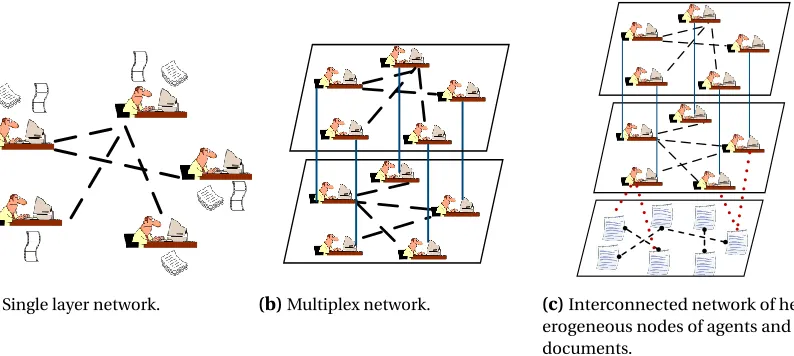
Figure 2.1 a) A single layer network between bloggers. Dashed edges show connections between blog-gers. b) A multiplex network between blogblog-gers. The top layer is based on the hyperlink
inter-connectivity of the bloggers, and the bottom layer is the friendship network between the bloggers. The straight inter-layer edges are showing that the bloggers are the same people in both layers. c) An interconnected network of heterogeneous nodes of agents and
docu-ments. The dotted edges are showing which blogger (agent) has produced which document. A similar set of dotted inter-layer edges are present from the top layer to the bottom layer which has not been depicted in the picture. . . 6 Figure 2.2 The interconnected networkI(Eqn. (2.2)) with two agent-layers and one information-layer.
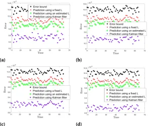
A set of inter-layer edges (similar to the red lines) are present from the top layer to the bottom layer which have been excluded in the picture for simplicity.. . . 11 Figure 2.3 The effect of different magnitude ofΣAmatrix on the state of agents. . . 15 Figure 2.4 Experiment for college researcher network with 1000 publication documents. 20 Figure 2.5 Experiment for a Twitter network with 1000 agents and 8 Hashtags. . . 21 Figure 2.6 Experiment over Twitter network with 5000 agents and 8 Hashtags. . . 22 Figure 2.7 Experiment over the Twitter network with different sizes. . . 23 Figure 2.8 Experiment over Twitter network with 300 agents. Predicting the states of
agents using a fixed Laplacian matrix, using an estimated Laplacian matrix, and Prediction using Kalman filter with 10 percent, 15 percent, 20 percent, and 25 percent of observation of states of all the agents in Figs. (a), (b), (c) and (d) respectively. . . 24 Figure 2.9 Comparing the estimated value of the second smallest eigenvalue with the
actual second smallest eigenvalue of the interconnected network. . . 25 Figure 2.10 The effect of weak inter-layer connectivity on the state prediction error. . . . 25
Figure 3.1 Sequential steps of a deep dictionary withslayers. . . 31 Figure 3.2 XandAare respectively, the images and the associated feature vectors.Y
represents the class labels, and ˆY is the estimated class labels by the classifier. 35 Figure 3.3 Mutual informations of output of each layer with the input signal . . . 36 Figure 3.4 Effect ofγon the second moment of the sparse repersentation. . . 39 Figure 3.5 Reconstruction error with varyingγ. . . 39 Figure 3.6 Changes in the classification accuracy of the proposed method on the
CIFAR-10 dataset over different epochs. . . 43 Figure 3.7 comparison between the reconstructed images form DDL and the original
images form CIFAR-10 dataset . . . 44 Figure 3.8 Fooling rate in MNIST dataset . . . 45 Figure 3.9 Fooling rate in CIFAR-10 dataset . . . 46 Figure 3.10 Learning curves of the proposed method with different number of layers on
the CIFAR-10 dataset. . . 46
Figure 4.1 Sequential steps of a sparse generator network. . . 53 Figure 4.2 Generating and encoding images. Blue/red squares and circles represent
CHAPTER
1
INTRODUCTION
It is a fact that a great variety of topics may typically prevail in social networks, and their diffusion
entail distinct dynamics which also imply that the agents are differently affected. The temporal and spatial dynamics of diffusion have been studied through sequences of activation nodes and
observed or modeled as spreading cascades in a network[43].
The information diffusion process models can be classified into three major groups, probabilistic models, thermodynamic models, and counting models. NETINF[34], NETRATE[91]and INFOPATH [35]are the probabilistic models which infer the underlying diffusion network among information sources using consecutive hit times of the nodes by a specific cascade. The main idea behind the thermodynamic models[30, 33, 81, 99]is that heat will propagate from a warmer region to a colder region, or gas will move from the region with higher density to the region with lower density. The
counting models[50], on the other hand, form counting processes to find the number of nodes in each group of susceptible or infected nodes. SIS[80]and SIR[96]are two well-known models in this group.
One central challenge in modeling information diffusion is to understand the structure of the cascades; the existence of unknown external influence factors and unclear graph connections
obscure this query. In Chapter 2 of this sequel, we propose for the first time, to model the simple diffusion on a general multilayer network, and apply the model to publication networks and social
media data. In particular, we propose alayered and interconnected networkto move beyond a two-layer network, as has appeared in the literature[33]. This in turn, allows diffusion to occur over many layers (a trulymulti-layer diffusion network).
A multilayer network takes into consideration additional connection criteria when the true
of documents generated by bloggers over time; these documents may share some topical similarities
in spite of their diverse sources. It is possible to structure the document similarities into a relational property captured by a network of documents. One can then further augment this connectivity layer
with an associated connection of bloggers (e.g., according to following-follower connection). This
leads to a multilayer network model where information diffuses both within a single layer and across layers. The additional paths due to the multilayer structure, diffuse the information at a secondary
degree, specifically, an absence of a direct connection between two bloggers may be reestablished by
counting the topical similarities between the documents they are associated with. We thus propose, in Chapter 2, a multilayer construction of interconnected network of heterogeneous nodes to model
the diffusion process in online social networks. In a community-like network of agents with common
interest, such as a network of authors with their publications, an online forum community, we have observed thermodynamical-like diffusion patterns. It turns out that the simple diffusion model on
the interconnected network structure is very effective in predicting the future states of the agents.
In the third Chapter of this thesis, we explore the structure of data (potentially any class) to develop strategies for improved inference. We note that the current state-of-the-art for high
di-mensional data analysis is deep learning based on neural networks, which unfortunately remains,
to a large extent, a black-box technique. The well-known problems with deep learning include brittle performance in the presence of uncertainties, and the lack of insight; it is impossible to know
how a conclusion is reached and why. Therefore, in Chapter 3, we propose techniques towards overcoming some of these deficiencies by analyzing high-dimensional data such as images. For this
data modality, Deep Neural Networks and Dictionary Learning for Sparse Representation figure
among the two most well-known research directions in feature retrieval and inference with image data.
Sufficient experimental evidence has shown over the last few years that Deep Neural Networks
(DNNs), and more specifically Convolutional Neural Networks (CNNs)[18, 61], have been nothing short of impressive in many applications, including signal and image processing[26, 108]. A Con-volutional Neural Network consists of multiple layers, each with different number of filters. These
significant achievements, have, however, not been matched by a deep theoretical understanding of their underlying functionality and design.
On the other hand, the application of Occam’s razor in the parsimonious data representation
by using overcomplete dictionary learning has shown promising results in a variety of problems such as image denoising[29], image restoration[115], and image classification[120]. This frame-like representation of each data subset as a linear combination of atoms, carries a sparse notion of
associated coefficients. This potentially leads to a poor performance when the training dataset is small. Convolutional Neural Networks, however, learn the initial features from small image patches
and build a hierarchy of features at different scales. Contrary to conventional wisdom, deeper
have showed serious limitations in presence of adversarial perturbations[78]. To address some of these limitations and further explore the intrinsic deep structure of various data classes, we propose a principled hierarchical (deep) dictionary learning duly constrained by a classification objective
functional. To capture the scale relational information, the front layer dictionary is learned on small
image patches, and the subsequent layer dictionaries are learned on larger patches. Put simply, the initial scale captures the fine low-level structures comprising the image vectors, while the next
scales coherently capture more complex structures. The classification is ultimately carried out by
assembling the final and largest scale features of an image and ascertain their contribution. In contrast to CNN, we show that the performance of the proposed Deep Dictionary Learning (DDL)
method improves with additional layers, hence indicating an amenability to tuning, and a better
potential for more elaborate learning tasks such as transfer learning. This proposed approach is also demonstrated to exhibit robustness to additive noise and particularly to the so-called adversarial
noise.
Exploitation of deep structure information of the images, has also been shown useful for syn-thesizing new images from a set of real images using Generative Adversarial Networks (GANS)[36]. In Chapter 4, we propose a novel Generative Adversarial Networks (GANs) method by learning
the structure of images at smaller scales subsequently using the learned structures to synthesize full-scale images.
On account of numerous open issues, the GANs research is still in its infancy. The complex structure of real-world images, indeed causes GANs to fall short on consistently synthesizing realistic
images. Images are known to follow complex probability distributions and estimating these
distribu-tions at the full image scale is generally a difficult task. Mode collapse, a well-known phenomenon in GANs, where highly similar images are frequently generated from different inputs, is widely
at-tributed to the problem of complexity of the image distributions. To alleviate the above-mentioned
issues, we propose a novel generator model which learns the structure of images at smaller scales, and uses the learned structures to synthesize full-scale images. To this end, we adopt dictionary
learning and sparse representation[68], as an effective combined methodology to learn and leverage the structure of data.
Our proposed generator network yields a sparse vector of coefficients for each image patch
instead of generating the entire image. Full-size output images are assembled by tiling the image
patches, produced by multiplying the generated sparse coefficient vectors to a pre-trained dictionary. This approach avoids the complexities with the conventional method of generating the entire image
in one step. Instead, it affords a multi-stage solution, where in the first stage, simpler structures
are generated at the scale of image patches, and a full-size image is assembled in the final stage. Incorporating sparse representations also limits the search space of the produced images to a
linear combination of a set of dictionary atoms, tailored for representing real-world images, thus
enhancing the procedure of generating realistic images. To avoid the mode collapse problem, we also introduce a third player in the proposed GANs architecture which we refer to as the reconstructor.
dissimilar outputs i.e., the generator is an injective map. Second, it guarantees that the real images
in the dataset can also be synthesized from some input noise i.e., the range space of the generator includes the entire set of real images. These goals are achieved by treating the generator network
as a "decoder" from a latent input space which simultaneously trains an "encoder" network, that
reversibly computes the input of the generator from its output. The encoder function is a regularizer to the generator network, and is minimized successively along the generator and the discriminator
losses. Existence of such an auto-encoder scheme guarantees that the generator network is injective,
CHAPTER
2
INFORMATION DIFFUSION OF TOPIC
PROPAGATION IN SOCIAL MEDIA
2.1
Introduction
As a physical process, a network information flow—through its rather extensive connectivity and
resulting frequent exchanges among the nodes, as connecting entities—is a pervasive diffusion. The
high activity over a typical network entails active dynamics, and hence large variations in content. The states of agents (nodes) in such a network are consequently actively altered by the diffusion of
information, according to associated dynamical parameters of the network. Throughout this sequel,
we use the general term "agent" to refer to users in social networks, bloggers, also authors, or any individual who produces information content, and is networked with others. Agents in one network,
are typically interested in different topics. Bloggers, for example, may write about specific topics, while different authors may only publish articles about their own research areas. The interest of a
given agent may, also, evolve over time, as a result of diffusion of information from other agents or
sources. This work is, to the best of our knowledge, the first to address this problem.
In particular, we propose alayered and interconnected networkto move beyond a two-layer network, as has appeared in the literature[33]. This in turn, allows diffusion to take place over many layers (a trulymulti-layer diffusion network). A few recent works[3, 9, 20, 82, 83]have mathematically studied multilayer networks. To proceed, we note that the diffusion phenomenon in our later
formulation will also be useful in predicting the future states of agents in a network. Specifically, an
(a)Single layer network. (b)Multiplex network. (c)Interconnected network of het-erogeneous nodes of agents and documents.
Figure 2.1a) A single layer network between bloggers. Dashed edges show connections between bloggers. b) A
mul-tiplex network between bloggers. The top layer is based on the hyperlink inter-connectivity of the bloggers, and the bottom layer is the friendship network between the bloggers. The straight inter-layer edges are showing that the bloggers are the same people in both layers. c) An interconnected network of heterogeneous nodes of agents and doc-uments. The dotted edges are showing which blogger (agent) has produced which document. A similar set of dotted inter-layer edges are present from the top layer to the bottom layer which has not been depicted in the picture.
1) Information and State of Agents:
To successfully model the information diffusion, it is first imperative to carefully define the type of
dynamics which characterize the diffusion process. Many existing diffusion-based models[13, 15, 23, 74, 88, 92–94, 110, 125]focus on spread of infectious disease or social contagion on networks. In these models the infection can spread from any infected agent to its neighbors under certain
conditions and sets of probabilities, and the agents can either be in susceptible, infected or recovered
states.
Despite the subtle differences in these models, the state space of the agents is usually binary,
indicating influence from a certain information. While these types of diffusions may capture some
dynamics, they present serious limitations in any practical network settings. A case in point is that of a diffusion process due to a blogger’s read of other blogs in a network, and whose state/opinion changes as a result. This in turn, changes the dynamics of the network. In Instagrams, users may
"repost" each other’s images (with or without modification of the original image), thus implying that the information diffusing through the network may come from text, image, video, and other
types of documents.
2) The connectivity model:
Graphs are most commonly used to model the connectivity among agents who are represented
by nodes, and whose connection is depicted by edges. In the aforementioned "bloggers" example,
connectivity between bloggers highlights the fact that they read each other’s blog. Fig. (2.1a) shows a single layer connectivity structure between the bloggers; but various structures between them are
also possible. We may, for instance, consider the information about the hyperlink connectivity as
structure (multiplex with two layers) between bloggers.
In this work we define the state of each agent as a feature vector. Specifically, we will consider the state of each agent as a topic vector, reflecting the extent to which an agent is associated with
specific topics. Our goals in this endeavor are: creating a multi-layer diffusion network among
agents and information contents, estimating the future state of agents, learning the structure of the supra-Laplacian matrix from previous diffusion history, and predicting the ensuring future states
assuming that a partial observation of the states of agents is available.
We go beyond the two-layer case to account for topical connectivity among the content nodes (sources of data characteristic of the information permeating the interconnected network) thus
yielding a multi-layer network. In our example, blogs consist of a set of documents generated
by bloggers over time, as illustrated in Fig. (2.1c). These document sets may share some topical similarities (despite their distinct blogger sources). Structuring these relational properties into a
network of document sets, introduces additional connecting edges between agents and document
sets, as well as among agents. These additional paths will diffuse information at a secondary degree, specifically, an absence of a direct connection between two bloggers, does not exclude one blogger
getting updated on another blogger, and this on account of topical similarities between associated
documents. We will refer to this complex structure of connected networks, as aninterconnected networkof heterogeneous nodes, with advantages further discussed in Section 2.3. This structure will help us understand the process by which an author’s topical interests are changing from a topic to another, or why different topics are getting different amounts of attention by users in online social
networks.
While states of agents represent their current engagement in different topics, they will evolve over time to reflect newly produced documents, hence updating the agents’ states. We propose to
estimate the state of the agents at timet1, knowing their state upto timet0<t1with the help of
the interconnected network. This is accomplished by considering a multi-layer diffusion network among the agents and documents.
In many cases, the actual diffusion among the agents is different from the fixed connectivity
which we observe in the network (e.g, for a given friendship network between bloggers, a connection between two friend bloggers does not necessarily imply an influence of one on the other.). By
ob-serving diffusion related patterns over a short period of time, we particularly attempt to understand
such astaticinfluence network (reasonably for a short time interval), which has the presumably close connection to agents involvement in some common interest, with the capacity of leading
to a common consensus. To that end, we learn the structure of the supra-Laplacian matrix of the
underlying network of influence, which we subsequently use in our prediction phase.
In certain online social networks, one often encounters a set of conservative users with strict
privacy policy, and a fraction of hub nodes with public information, and this clearly alters the
previously designed state prediction problem. We exploit the flexibility of the Kalman filter to address the problem, assuming that a partial observation of the states of agents is available. The
available states.
The remainder of the chapter is organized as follows: In Section 4.2 we discuss some background and related work to our contribution. Section 2.3 describes our basic formulation of the problem.
We propose our new approach in Section 2.4, and present substantiating experimental results in
Section 4.5. We provide some concluding remarks in Section 2.6.
2.2
Related Works
A mathematical investigation of multilayer networks has been extensively conducted in a series of recent papers: In[20], modularity of multilayer networks has been defined through tensor based modeling of connections; in[3, 9]a number of metrics are introduced and defined to characterize multilayer networks structurally and dynamically. In recent years, a number of studies of real-networks have also focused on epidemic spreading in multiplex real-networks. In[112], and[19]two epidemies spreading in a layered multiplex network were addressed. While agents in the
two-layered multiplex network are the same, their connectivity structures are different. In[33], the associated authors discuss the diffusion dynamics in such a network. The authors introduce a
supra-Laplacian matrix, and used a perturbation analysis to study the effects of changes in the
spectral properties of a single layer on the spectral properties of the whole network. The nodes in different layers of the model proposed by[33]have one-to-one connection between each others. Similarly in[31], the authors study the spreading of two different processes in a multiplex network. Their work mostly focused on the impact of the degree correlation of the two layers on the epidemic properties of the processes. The state space they considered, similar to many others, was of binary
nature (infected or not-infected) to model the spreading processes.
Note that one may classify the information diffusion process models into three major groups, probabilistic models, thermodynamic models, and counting models. NETINF[34], NETRATE[91]and INFOPATH[35]are the probabilistic models which infer the underlying diffusion network between information sources using consecutive hit times of the nodes by a specific cascade. The diffusion network, in this case, was the result of solving an optimization problem which is computationally
very expensive (super-exponential). The main idea behind the thermodynamic models[30, 33, 81, 99]is that heat will propagate from a warmer region to a colder region, or gas will move from the region of higher density to the region of lower density. Modeling the information as heat or gas, we
can write the rate at which information varies for agentias: dψi d t =D
P
jA(i,j)(ψj−ψi),ψi(t)is the state of theit hagent at timet, whereD is a diffusion constant which is the amount of information passing from one agent to another agent in an infinitesimal interval of time, andA(i,j)is the(i,j)t h
entry of adjacency matrixA. The counting models[50, 80, 96]form counting processes to find the number of nodes in each group of susceptible or infected nodes. Assuming that each agent hasβ
contacts per unit time with other agents, and in each contact of an infected agent with a susceptible
respectively. We therefore, can write the rate of change ofX andSasd Xd t =βS Xn andd Sd t =−βS Xn .
Building on these prior information diffusion models, we address in this chapter the following limitations.
A)Almost all existing information diffusion models are based on the contagion principle, using an abstract term or a clear data tag. Specifically, many information diffusion models in social networks, for example, consider a specific "Hashtag" or repost as contagion[30, 33, 34, 99]. We would, thus, need to advance existing information diffusion models, if one were interested in, tracking
the way bloggers influence each other, or how articles and related research fields vary over time, or parsing through very large multi-modal data sets.
B) A few information diffusion models[33, 99]have recently considered multiplex connectivity models. The overwhelming majority of these works model the connectivity by just using simple graphs. Agents may, however, display several forms of connectivity, through multiple online social
networks, or other social clubs, thus making simple graph models highly biased for capturing the
real world complexity of information diffusion models.
C) Even though a few works consider information diffusion in presence of an external input[39], most of the existing models are layered without possible external perturbations/inputs. Specifically, considering the bloggers’ example, the documentation evolves with time, and so do the nodes of the network, hence impacting the mutual influence the agents have on each other. This is indeed key to
one’s ability to proceed to any future state prediction on the network. In the present work, we model each agent state vector as a topic vector, effectively as a topic proportion associated with the agent’s
own documents. In so doing, our solution predicts the users’ future topic vectors by considering
their interactions inside the interconnect network agents, as well as those of the documents. This network is allowed to vary over time on account of both the diffusion effect, as well as that of external
inputs as new documents are added.
Our work bares some similarity to the research in[33], we additionally, consider the intercon-nected network of heterogeneous nodes of documents and agents (Fig. 2.1c) rather than the simpler
multiplex network (Fig. 2.1b) in[33]. We also generalize the scalar state space of agents to a higher dimensional state space of topic proportions. Furthermore, we consider, in this sequel, an open system, and study the external effect on each agent from the agents or documents which have not
been captured by the diffusion in the network.
2.3
Problem Formulation
We represent agents within a social network setting, by nodes on a graph, and their connectivity by edges between them. The connectivity may reflect friendship, co-authorship, or other forms of
behavioral similarities. If we consider a setVA ofN agents, we can imagineMA different graphs
Table 2.1Terminology
Symbol Definition Symbol Definition
A,I Agents & documents resp. W(Ak) Intra-layer connectivity matrix of agents in layerk.
Ai,Ip Agenti& documentspresp. W( k,m)
A,I Inter-layer conn. of layerktomamong agents and docs. GA(m),GI(m) Intra-layer graphs of layerm. DA(k) Intra-layer diffusion constant of the agents in layerk.
I The interconnected graph. DA(k,l) Diffusion constant of agents from layerktol.
T Length of the topic vectors. DA(k,I,m) Diffusion const. of layerktom. among agents and docs.
L(m) Laplacian matrix of layerm. N,S,P # of agents, documents & all nodes resp.
x(Am)
i State of agentiin layerm. L Supra-Laplacian matrix.
xIp State of documentp. X AP×Tmatrix consisted of the state of all nodes.
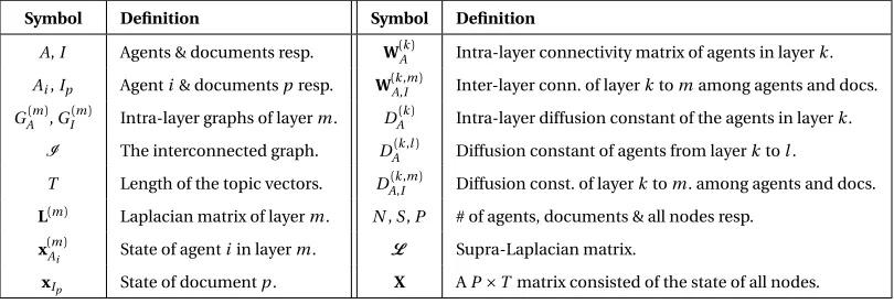
communicating agents. In Fig. (2.2) we can see two agent-layers. We note in this case, that the agents are the same in both layers, and we hence have a direct one to one connections between them (the
blue edges in Fig. (2.2)).
Agents are usually assumed to possess some data or to produce information in their embedding network. If, for instance, the agents were bloggers or social network users, they would be producing
blog-documents or their online accounts, if they were researchers, they would be turning out scientific papers. These sets of documents, may also mutually store topical similarities which will
play a role in the overall information diffusion throughout the network. Of central interest in our work,
is the evolution of the topical states of the agents, as the information diffusion takes place. Latent Dirichlet Analysis (LDA)[8], Latent Semantic Indexing (LSI)[21]and several other topic modeling algorithms afford us the ability to represent any text document as a state vector of lengthT.T is an
arbitrarily chosen number of topics (dimension) in a collection of text documents. Considering the documents as vectors in aT−dimensional vector space, we can build a similarity network between
these vectors using their euclidean inter-distances, as well as a neighborhood criterion between them
(e.g.K-Nearest Neighbors algorithm, Epsilon-Neighborhood). We consider a setVI ofSdocuments. The subscriptI specifies the information nature of the network and of its members (i.e, it pertains
to documents in this case), withMI different graphsGI(m)= (V
(m) I ,E
(m)
I ),m=MA+1, ...,MA+MI, each describing a different connectivity structure amongS documents (the bottom layer in Fig. (2.2)). Note that similarly efficient tools (e.g. ISOMAP[103], Principal Component Analysis (PCA) [55], Multi-Dimensional Scaling (MDS)[105]) for dimension reduction are available for multi-modal documents (images, videos, ...), to possibly represent them as separate networks. In this work, we refer to the network among the documents as the information-layer. Table 2.1 lists all notations
used in this chapter along with their definitions.
By adopting an adapted notation of[58], we represent the documentp byIp, and the agent i byAi. The red inter-layer edges (EA,I) in Fig. (2.2) relate agents to their respective documents
(publisher-publication network). The information of documentIpis denoted by aT dimensional
Figure 2.2The interconnected networkI (Eqn. (2.2)) with two agent-layers and one information-layer. A set of inter-layer edges (similar to the red lines) are present from the top inter-layer to the bottom inter-layer which have been excluded in the picture for simplicity.
vectors of their associated documents:
x(Aim)= 1 |NI(Ai)|
X
p∈NI(Ai)
xIp, (2.1)
whereNI(Ai)is the set of documents produced by agentAior more formally, the neighbor set of agentAi in the information-layer, which|NI(Ai)|is the cardinality of that set. The interconnected graph in Fig. (2.2) may thus be denoted by:
I=VA(1)∪VA(2)∪VI(3)
, EA(1)∪EA(2)∪EI(3)∪EA(1,2,A)∪EA(1,3,I)∪EA(2,3,I)
. (2.2)
With this inter-connected formulation, and in analyzing an associated information diffusion
process, we address in this chapter,
• The ability to achieve a diffusion of information between agents via multiple connectivity structures. The same set of agents may have different intra-layer connectivity at different
layers;
• The ability to model networked documents in a separate network layer, will enable us to
consider the similarities, and their evolution over time between the documents as an infor-mation diffusion medium. For instance, agentsAiandAj in Fig. (2.2) are not connected via
any paths through the top two agent-layersGA(1), andGA(2). There is, however, a path between
these two agents by way of the similarity of their documentsIpandIq inGI(3). The intuition supporting the interaction betweenAiandAj in the blogger’s example, follows from: blogger
L=
D(1)L(1)+D(1,2)I+D(1,3)K(1,3) −D(1,2)I −D(1,3)W(1,3)
−D(2,1)I D(2)L(2)+D(2,1)I+D(2,3)K(2,3) −D(2,3)W(2,3)
−D(3,1)W(3,1) −D(3,2)W(3,2) D(3)L(3)+D(3,1)K(3,1)+D(3,2)K(3,2)
. (2.9)
• The preservation of the conventional information diffusion structures such as the co-authorship
network in the introduced interconnected network model (e.g the agentsAj andAk who have collaborated to produce theIp).
2.4
The Proposed Method
In this section we address the information diffusion across agents as a result of topic adoption and adaptation, as well as external topic addition updates. To that end, we next consider a closed
interconnected network with no additions. In Section 2.4.2, we consider an open interconnected
network and account for an innovation injection. In Section 2.4.3, we define the estimation of the supra-Laplacian matrix using learning data. In Section 2.4.4, we further refine the predicted state
of the nodes using Kalman filtering. In Section 2.4.5, we analyze the effect of a weak inter-layer
connection on the over-all diffusibility of the interconnected network.
2.4.1 Closed system: Information diffusion in a heterogeneous network
In closed systems, all changes in the agents’ states are a result of interaction among the agents in
the network. In a single layer diffusion process[30, 33, 81, 99], an agent state maybe formalized as:
dxAi
d t =D
N X
j=1
W(i,j)(xAj−xAi), (2.3)
where dd txAi is theit hagent’s topic vector change over time.W(i,j)reflects the connectivity status
between agentsi andj, whileD is the diffusion constant, or the fractional amount of information
passing fromj toiin a small time interval. By further simplifying Eqn. (2.3), we may write dXA d t as follows:
dXA
d t +DLXA=0, (2.4)
whereXAis anN×T matrix, and rowiis denoted by the row vectorxTAi;Lis anN×N graph Laplacian
matrix (i.e.,L=K−W,Kbeing the diagonal matrix of the nodes’ degree).
Independently of the type of nodes in the network, we can state the following,
Claim 1. Denoting the supra-Laplacian matrix of an M layer multiplex network with N nodes in each layer given Eqn. (2.5), withLL as the supra-Laplacian matrix of the intra-layer connectivity,
andLI as the supra-Laplacian matrix of the inter-layer connectivity, the following maybe written:
LL= M
M
α=1
D(α)L(α)=
D(1)L(1)
D(2)L(2) ...
D(M)L(M) . (2.6)
See appendix A for proof of Claim 1.
In addition, the inter-layer supra-Laplacian can be written asLI = PM
α=1(KαI −WαI), where the KαI is the diagonal inter-layer degree matrix of layerα, highlighting the inter-layer degree of the nodes in layerα, and theWαI as the inter-layer connectivity matrix of the nodes in layerαwith the nodes in the other layers. TheKαI andWαI are formally defined in Eqns. (2.7 and 2.8) respectively as,
KαI =E(α,α)⊗(
M X
β=1β6=α
D(α,β)K(α,β)), (2.7) WαI =
M X
β=1β6=α
(E(α,β)⊗(D(α,β)W(α,β))), (2.8)
whereK(α,β), is a diagonal matrix reflecting the degree of each node in the inter-layer connectivity between layerαand layerβ,W(α,β)quantifies the inter-layer connectivity of the layerαnodes to the layerβ nodes, andE(α,β)is an all 0,M ×M, matrix with an only 1 element in(α,β).
Claim 1 shows that in a multilayer network setting, that by denoting the changes in nodes state as dX
d t =−LX, the supra-Laplacian matrixL, is given by Eqn. (2.5). Comparing the results in[33]with the above definition of supra-Laplacian matrix, Claim 1 formulates the definition of supra-Laplacian
matrix for a general multilayer network with an arbitrary number of one-to-one layers and a general
inter-layer connectivity. Following is an example which further details steps of the proof.
Example 1. In a three-layer interconnected network similar to Fig. (2.1c),Xis a P×T matrix (P=
2N+S ) which represents the states of agents in the top two layers (X(1)andX(2)), and of the topic vectors of documents in the third layer (X(3)). Following the terminology in[33], we refer toL as a
supra-Laplacian matrix, by its ability to capture the diffusion in inter-connected network system. Assuming
undirected graphs in each layer, and symmetric diffusion constants (D(k,m)=D(m,k)), we can write
for easier explanation, the supra-Laplacian matrix in case of a three layer-network (Fig. (2.2)), with two agent-layers and one information-layer as Eqn. (2.9). For this specific a 3-layer inter-connected
network, we simplify our notation by dropping the subscripts (as in Eqn. (2.9). Specifying the nature of a network layer) in favor of superscripts.1This hence makes matrixLmrepresent the Laplacian of
the intra-layer connectivity matrix of layer m ,Ithe identity matrix, whileKmis a diagonal matrix
of node degree of layer m , andKm,n is a diagonal matrix reflecting the degree of each node in the inter-layer connectivity between layer m and layer n . This hence yields Eqn. (2.9), where the first
elements in the diagonal entries, formLL (Eqn. (2.6)), the other two elements in the diagonal entries
formKαIs (Eqn. (2.7)), and the rest (off-diagonal entries), formWαIs (Eqn. (2.8)).
2.4.2 Open System Diffusion: Impact of External Effects
Much of the existing work in information diffusion models have a limited scope (of agents, docu-ments, parameters) when predicting the future state of the nodes. More specifically, agent states
may be varied by external sources which are not captured in the network, or by some agents’ actions
which may even to some extent, conflict with the model prediction. In addressing the additional auxiliary input, we propose an open system model as follows:
First, consider a single layer network (agent-layer) for simplicity, we can then model the rate of
change in the state of nodei as follows,
dxAi=D N X
j=1
W(i,j)(xAj−xAi)d t+σidB(t), (2.10)
whereW(i,j)quantifies the connectivity between agentiand j, andD is the diffusion constant
reflecting the infinitesimal amount of information passing fromitojin a small interval of time, and B(t)is aT ×T matrix, whose columns areT-dimensional vectors with components as independent
standard Brownian motions of variancesσi. Inspired by the Ornstein-Uhlenbeck (O.U.) process [107], Eqn. (2.10) describes the velocity of the topical-state of the nodes as a Brownian motion in presence of friction. In other words, to describe the uncertainty due to external effects, we proceed
to view the whole system as a massive Brownian particle. The drift term (first term in right-hand side
of Eqn. (2.10)), however, moves the velocity from a martingale state ofσidB(t)towards a consensus (captured by the drift term). In matrix form, Eqn. (2.10) may be written as,
dXA(t) =−DLXA(t)d t +ΣAdB(t), (2.11)
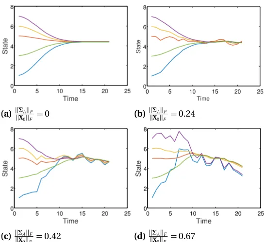
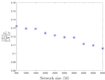
whereΣAis anN×T matrix, and each row shows theσivector in Eqn. (2.10) for agenti. Fig. (2.3)
shows numerical of examples of Eqn. (2.11) withN=5 andT =1. TheΣAmatrix adjusts the effect
of the consensus and the Brownian motion in Eqn. (2.11). In this figure, we have used the term ||ΣA||F
||X0||F (withX0=XA(0)) to compare the effect ofΣAmatrix magnitude on the states of the agents. As
the value of ||ΣA||F
||X0||F increases, the second term on the right-hand side of Eqn. (2.11) will have more
influence on determining the states of the nodes and consequently, the states of the agents will be changed by higher variability.
To extend to an interconnected setting, we can state the following statement: Given the states of
nodes at timet0we can predict the states at timet1,t1>t0as follows:
b
X(t1) =e−L(t1−t0)X(t0) +
Z t1
t0
eL(s−t1+t0)ΣdB(s), (2.12)
wheree−L(s−t1+t0)is a matrix exponential ofP×P size andΣisP×T matrix. To this end, we rewrite
Eqn. (2.11) for interconnected networks as,
0 5 10 15 20 25 0 2 4 6 8 Time State
(a)||ΣA||F
||X0||F =0
0 5 10 15 20 25
0 2 4 6 8 Time State
(b)||ΣA||F
||X0||F =0.24
0 5 10 15 20 25
0 2 4 6 8 Time State
(c)||ΣA||F
||X0||F =0.42
0 5 10 15 20 25
0 2 4 6 8 Time State
(d)||ΣA||F
||X0||F =0.67
Figure 2.3The effect of different magnitude ofΣAmatrix on the state of agents.
The first term on the right-hand side of Eqn. (2.13) describes the network-level diffusion taking
place among the nodes (mean reverting term), while the second depicts the global diffusion process,
affecting nodes regardless of their interactions. There are multiple ways to calculate the termRt1
t0 e
Lτdτ, one may use the basic definition of
a matrix exponential, and calculate the numerical value of the integral, or instead use the Jordan form asL=MJM−1andeLτ=MeJτM−1.
Our proposed learning procedure aims at determining the diffusion constants in the
supra-Laplacian matrixL as well as theΣmatrix. To that end, we proceed to minimize the Frobenius norm of the difference betweenXand its predictedXb,
arg min
Σ,D1,..
g=||X(t1)−Xc(t1)||F. (2.14)
Solving this optimization problem helps us decompose the predicted matrix into two main
com-ponents on the right-hand side of Eqn. (2.12), the first term representing the interactions in the network, while the second quantifying the variability which results from auxiliary inputs into the
system.
2.4.3 Diffusion Network Estimation (Learning the Supra-Laplacian Matrix)
The supra-Laplacian matrixL which we use in Eqn. (2.13) for state prediction, is the result of the network connectivity (refer to Eqn. (2.9)). In practice, hidden connections are pervasive, introducing
diffusion. To that end, consider observations ofX(t)overt ∈[0,t1], and denotex(t):=v e c(X(t)),
the vectorization ofX(t)to obtain a vector differential system in order to learn the supra-Laplacian matrixL of Eqn. (2.13):
˙
x(t) =Λx(t) +w(t), 0≤t ≤t1,
whereΛ=IT⊗(−L), the Kronecker product ofT-by-T identity matrix with(−L), andw(t)is the
vectorization ofw(t) =Σdd tB(t).
To that end, let the simple cost functional J =12T, where=x−xˆ, and estimating ˆΛ, using ˙ˆ
Λ=γ(x−xˆ)xT (derivative ofJ with respect to ¯x), to yield the estimation ˆx(t+1) =eΛˆx(t), whereγ >0 is appropriately chosen as the scaling gain. The optimization iterations lead to the estimated value
of ˆΛat theit hiteration as:
ˆ
Λi=Λˆi−1+Λ˙ˆi−1.
We use ˆΛ0=IT⊗(−L), the graph Laplacian of the explicit following-follower network (as initial-ization). The learnedΛmay not however, be exactly structured asIT⊗(−L), due to dependence
of topics in the state space, as well as the nonlinearity and non-homogeneity of the diffusion. The
resulting errorshall be considered for the estimation of the noise in the Kalman-Bucy filter as discussed next.
2.4.4 A Refined Prediction: Kalman-Bucy Filtering
In prediction applications, the actual states of some of the nodes may sometimes be known, and
we seek to predict those of all remaining nodes. An example of this may be seen in social networks, where states of the hub nodes, such as famous people or users with less restrictive privacy policies
are known to the public, and one is interested in predicting the states of other less accessible users.
Having partial knowledge of the states of a fraction of the nodes in the network, changes the state prediction problem to a Kalman predictor problem, and helps refine the predicted states using a
Kalman filter. We propose a Kalman-Bucy filter as the optimal linear predictor for our system, and
write the observation equation asy(t) = (IT⊗H)x(t)+v(t), withHas a diagonal indicator matrix with 1 in all the observed entries, and 0 in all other entries.Λhaving been learned (see above Section),
Kalamn-Bucy equations maybe written as:
˙
x(t) =Λˆx(t) +w(t),
y(t) =Hx(t) +v(t),
whereH =IT ⊗Hand the noisesw(t)andv(t)are zero-mean white (temporally) processes, i.e,
equation as ¯x(t +1) =Fˆx¯(t) +w¯(t), where ˆF=I+Λˆ:
x(t +δt)'x(t) +δtx˙(t),
x(t+δt)'x(t) +δt(Λˆx(t) +w(t)),
x(t+δt)'(I+δtΛˆ)x(t) +δtw(t).
Discretizing the Kalman-Bucy equations, yields the following discrete time equations:
¯
x(t +1) =Fˆ¯x(t) +w¯(t), (2.15)
y(t) =Hx(t) +v(t). (2.16)
Having Eqns. (2.15 - 2.16) as the state and observation equations respectively, we can predict
and refine the predicted states of the nodes using Algorithm (3):
Algorithm 1 Learning phase:
1: x(t)←v e c(X(t))
2: Λˆ←IT⊗(−L) .Initial state.
3: repeat:
4: xˆ(t +1)←eΛˆx(t)
5: Λ˙ˆ←γ(x−xˆ)xT
6: Λˆ←Λˆ+Λ˙ˆ
7: until||x−xˆ||2< η. .Convergence criteria.
Kalman filter prediction on test data:
1: Re,t←Rt+HΠt|t−1HT .Updating.
2: xˆ¯t|t←xˆ¯t|t−1+Πt|t−1HTR−e,1t[y¯t−Hxˆ¯t|t−1] 3: Πt|t←Πt|t−1−Πt|t−1HTR−e,1tHΠt|t−1 4: Fˆ←I+Λˆ
5: xˆ¯t+1|t ←Fˆxˆ¯t|t .Predicting.
6: Πt+1|t =FˆΠt|tFˆ T
+Qt
The "learning phase" of Algorithm (3) is estimating the supra-Laplacian matrix ˆΛ(see above Section). The second phase of the algorithm, is refining the estimated state of the nodes. Note that
Rt is the covariance of the observational error, and ˆ¯xt2|t1denotes the linear prediction of ¯xat time
t2given observations up to and including timet1. The filter equations of a Kalman-Bucy filter[56],
lines 1-3 of the algorithm, are given by:
˙ˆ
x=Λˆxˆ+Gt(y(t)−Hxˆ(t)), (2.17)
where theGt is the Kalman gain, while the state covarianceΠt satisfies theRiccatiequation:
˙
Πt=ΛΠˆ t+ΠtΛˆ T
+Qt−GtRtGTt . (2.19)
For simplicity, we further assume that the errors in the state prediction and observation are Gaussian
processes.
The designed algorithm shows the discrete time, state update of the Kalman predictor. The estimated states of the available nodes,Hxˆ(t), are compared with the state of the available nodes,
y(t), as measurements observed over time, to evaluate the extent of statistical noise and other
inaccuracies in predicting phase. The Kalman gainGt, is tuned to assign accurate gain on the measurement (state of the available nodes) or follow the prediction model (estimating the state
of the unknown nodes) more closely. More simply, the algorithm recursively learns from the error resulting from the estimation of the states of the available nodes and– by taking into account of the
covariance of the measured error– refines the estimation of the states of the less accessible nodes.
The time complexity of the proposed algorithm is dominated by the time complexity of matrix inversion of R matrix. Therefore, the time complexity class of the algorithm isO(n3).
2.4.5 Inter-layer Connectivity: Structural Robustness of an Interconnected Network In an interconnected network setting, the inter-layer links play a crucial role in speed of diffusion
between layers. Strong inter-layer links will cause a faster information diffusion among the layers, while, weak inter-layer connections will cause a set of independent layers[12, 99]. In this section we use perturbation theory[5]to study the effect of weak inter-layer linkage on the connectivity of the over-all interconnected network. The second smallest eigenvalue of a Laplacian matrix (algebraic connectivity) helps us to uncover how close the interconnected network is to breakup into multiple
connected components[16, 76, 99]. To this end, we claim following proposition,
Proposition 1. For an interconnected network (with connected intra-layer networks) with weak inter-layer links, the second smallest eigenvalue of the supra-Laplacian matrix of that network is
equal to,
εuTnLIun, (2.20)
whereunis an eigenvector of the intra-layer supra-Laplacian matrixLL,εis a small positive number.
The network is said weak, if the second smallest eigenvalue of its Laplacian matrix is close to zero.
See appendix B for the proof Proposition 1.
2.5
Experiments
To evaluate and substantiate the theoretical interconnected-network model proposed above, we
conduct discrete-time simulations of our system in both "closed and open" system conditions.
2.5.1 Data Sets
Our experiments have been carried out using the following data sets,
• Network of researchers and publications(N∼100):We assume a three-layer network, with two agent-layers for the researchers (the first and the second layers) and one
information-layer for publications (the third information-layer). In this data-set, the agents are 79 researchers at North
Carolina State University, and the documents are 1000 abstracts of academic papers published from 1990 to 2014. The agents in the first and the second agent-layers are the same individuals
with one-to-one connections between the agents. The first agent-layer is based on the
num-ber of papers two researchers have co-authored in the same venue.W(i1,)j is the cumulative sum of papers published by researcheriand j in the same venue. The second agent-layer
reflects research group co-membership of two researchers (with 8 different research groups considered).
W(i2,)j =
1 If researcheri andjare in the same group,
0 Otherwise.
(2.21)
The third layer (the information-layer) is based on the topical similarity of the produced
documents, and is quantified by the inverse distance between the topical vectors(T =10)of
the documents. Anε-neighborhood criterion has been applied to break the weaker links,
W(i3,)j =
1
||x(i3)−x(j3)||2
If larger thanε,
0 Otherwise.
(2.22)
T =10 dimensional topic vectors of documents have been produced by performing the LDA
topic modeling algorithm[8]on the raw text documents.
• Network of Twitter users and Hashtags(N =1000):A two-layer network of Twitter users,
(first layer) with(N =1000)users and the similarity network between eight different popular
Hashtags used by the Twitter users in June 2009. The Hashtags are as follows: #jobs, #spymaster, #neda, #140mafia, #tcot, #musicmonday, #Iranelection, #iremember. The agent-layer network
is a directed graph, based on who is following whom on Twitter. In our experiment we have
changed the directed edges to undirected ones, and states of agents are topic proportional vectors showing interest of agents in each Hashtag. The information-layer network is the
similarity network between the Hashtags, where two Hashtags are considered similar if both
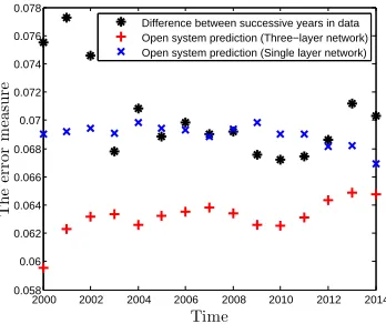
2000 2002 2004 2006 2008 2010 2012 2014 0.058 0.06 0.062 0.064 0.066 0.068 0.07 0.072 0.074 0.076 0.078 Time T h e e r r or m e as u r e
Difference between successive years in data Open system prediction (Three−layer network) Open system prediction (Single layer network)
Figure 2.4Experiment for college researcher network with 1000 publication documents.
network between the Hashtags, and theε-neighborhood criterion has been applied to break
the weaker links.
W(m2),n=
|Tweets which have both m and n|
|Tweets which have m or n| If greater thanε.
0 Otherwise.
(2.23)
• Network of Twitter users and Hashtags(N =5000):An exactly similar setting as the previously
mentioned data set, withN =5000 users.
2.5.2 Analysis of Results
Fig. (2.4) shows the results of our experiment on this data set (the network of researchers and
publications). The x-axis represents time, (and more specifically the consecutive years from Year 2000 until Year 2014). In our experiment, our goal is to predict the topical states of all the agents in
each year, using the topical states of agents in the previous year. More formally, we seekbX
(1)
(t)given
b
X(1)(t −1).
E r r o r m e a s u r e(t) =||Xb
(1)
(t)−X(1)(t)||
F
||X(1)(t)||F
, (2.24)
whereX(1)(t)is the ground truth matrix. The data over years 1990-1999 are used to learn the diffusion
constants, and those from years 2000-2014 for testing. The graph in blue Fig. (2.4) is the prediction errors by just considering a single-layer co-authorship network of agents/researchers. To be fair when comparing the multilayer networks with single layer networks, we have selected the
co-authorship network as our single layer because that was resulting in the smallest error compared to
co-membership network. The graph in red reflects the prediction error by considering a three-layer interconnected network of the heterogeneous nodes (as described in Section 2.5.1). The graph in
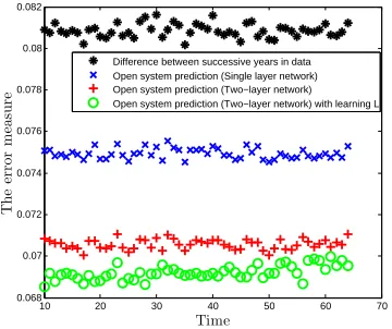
10 20 30 40 50 60 70 0.068 0.069 0.07 0.071 0.072 0.073 0.074 0.075 0.076 0.077 0.078 Time T h e e r r or m e as u r e
Difference between successive years in data Open system prediction (Single layer network) Open system prediction (Two−layer network) Open system prediction (Two−layer network) with learning L
Figure 2.5Experiment for a Twitter network with 1000 agents and 8 Hashtags.
the difference in the yearly topical states of agents, as in,
||X(1)(t)−X(1)(t−1)||
F ||X(1)(t)||F
. (2.25)
Eqn. (2.25) is an upper bound of our prediction error, and any reasonable prediction method should
have a smaller error than the the one in Eqn. (2.25). We may indeed just assume no change in the agent states has occured to achieve the error in Eqn. (2.25).
2.5.2.1 Prediction using single layer network vs. heterogeneous network
Network of researchers and publications(N ∼100):As may be seen in Fig. (2.4), the prediction
method based on a three-layer network achieves a lower error than the prediction based on a
single-layer network. Note that the single-single-layer network does not help in predicting the topical states of agents. The reason is that there are only 79 agents in this experiment, and the co-authorship network
between the agents is not particularly suited to predict the future states of agents. The three-layer
network, on the other hand, considers the similarity between the documents present in the network, and accounts for more elaborate diffusion paths, thus enhancing the prediction phase. The average
prediction improvement by the three-layer network over that of a single-layer network is 8 percent.
If we increase the number of documents and keep the number of agents fixed, the error decreases. Network of Twitter users and Hashtags(N=1000):Fig. (2.5) displays the results of our
experi-ment on the second data set. The time (x-axis) reflects intervals of consecutive six-hour periods.
In this experiment, recall, our goal is to predict the topical states of all agents at each time point when given the topical states of agents at previous time points. The error metric is similar to that in