Distributed Parameter-Dependent Control of Non-Uniform Flexible Structures

(1)

Abstract

Yildizoglu, Suat Ege. Distributed Parameter-Dependent Control of Non-uniform Flexible Structures. (Under the direction of Dr. Fen Wu)

(2)

DISTRIBUTED PARAMETER-DEPENDENT CONTROL

OF NON-UNIFORM FLEXIBLE STRUCTURES

by

Suat Ege Yildizoglu

a thesis submitted to the graduate faculty of

north carolina state university

in partial fulfillment of the

requirements for the degree of

master of science

department of mechanical and aerospace engineering

raleigh

July 2002

approved by:

(3)

Dedicated to...

my parents Leman and Sava¸s my sister Ece

and

(4)

Biography

(5)

Acknowledgements

I would like to express my deepest appreciation to my advisor Dr. Fen Wu for all his support, encouragement, availability and invaluable guidance throughout this re-search. I cannot thank you enough for your patience and generosity. It has been a great pleasure to work with you.

I would like to thank my committee members, Dr. Larry Silverberg and Dr. Paul Ro, for taking interest in my work and for their valuable time. I would like to take this opportunity to thank the Mechanical and Aerospace Engineering Department for the ﬁnancial support they provided.

I would like to give my appreciation to my fellow graduate students, Juan Jaramillo and Marco Soto for their kindness and friendship. I would like to extend my special thanks to Marco, who did the painstakingly proof-reading of this thesis. I wish you luck in the rest of your lives. I would also like to thank my roommate Fatih for his patience and support.

I would like to express my heartfelt gratitude to my parents, my aunt and my sister, who have always been there for me. I wouldn’t have been here without their invaluable advice and encouragement. Thank you mom and dad, for all the things you have done to provide me with the best possible opportunities in life.

(6)

List of Figures

2.1 Distributed parameter system . . . 13

2.2 Distributed control architecture . . . 16

2.3 Closed-loop LFT Framework . . . 17

3.1 Non-uniform ﬂexible cantilever beam . . . 26

3.2 Block diagram representation of equation (3.11) . . . 29

3.3 Deﬂection of the free end of the uniform beam, 1st mode excited . . . 36

3.4 Deﬂection of the free end of the uniform beam, 2nd _{mode excited . . .} ₃₇

3.5 Deﬂection of the free end of the uniform beam, 3rd _{mode excited . . .} ₃₈

3.6 Deflection of the free end of the uniform beam, combined modes excited 39 3.7 Deflection of the free end of the non-uniform beam, 1st _{mode excited} ₄₀ 3.8 Deflection of the free end of the non-uniform beam, 2nd _{mode excited} ₄₀ 3.9 Deflection of the free end of the non-uniform beam, 3rd mode excited 41 3.10 Deflection of the free end of the non-uniform beam, combined modes excited . . . 41

4.1 Weighted open-loop system for controller synthesis . . . 44

4.2 Modiﬁed distributed control architecture . . . 48

4.3 Case 1, Displacement of the free end, no disturbance . . . . 50

4.4 Case 1, Control input at the free end, no disturbance . . . . 51

4.5 Case 1, Displacement of the non-uniform beam, no disturbance . . . 51

4.6 Disturbance Input and Noise at the free end . . . 52

4.7 Case 2, Displacement of the free end, disturbance rejection . . . 52

4.8 Case 2, Control input at the free end, disturbance rejection . . . . . 53

4.9 Case 2, Displacement of the non-uniform beam, disturbance rejection 53 4.10 Case 3, Displacement of the beam at malfunctioning actuator location 54 4.11 Case 3, Displacement of the free end . . . . 54

4.12 Case 3, Control input at the free end . . . . 55

(9)

List of Tables

3.1 Non-uniform ﬂexible beam parameters . . . 28

3.2 First ﬁve natural frequencies of a uniform ﬂexible beam . . . 35

3.3 First ﬁve natural frequencies of a non-uniform ﬂexible beam . . . 38

(10)

Chapter 1 Introduction

The control of flexible structures has been one of the most active fields of research for the last two decades partly due to increased interest in high-speed robotics and space applications. In the construction of large space structures, for example, low-mass density materials need to be used due to the high launch cost. Since these materials are also lightly damped, the increased flexibility of space structures may allow large amplitude vibration, which may cause structural instability. In high-speed industrial robotics applications, however, the highly flexible nature of the links leads to a challenging problem of end-point trajectory control. Therefore, sophisticated controllers that enhance the stiffness and damping properties of these structures are needed to overcome these problems.

There are two main approaches for the vibration control: passive and active. In the passive method, the damping of the structure is increased by using passive dampers or materials with signiﬁcant viscoelasticity (see for example [21], [39]). Nevertheless, this method can increase the total weight considerably, which is not desirable in many applications. On the other hand, the developments in material science have led to a number of promising materials such as piezoelectric materials, which can transform electrical energy into mechanical energy, and vice versa, so that they can be used as sensor or actuator elements for active control of structural vibration.

(11)

vibration control of ﬂexible structures. In this chapter, a brief review of related research in literature is presented.

1.1 Background

Flexible structures are usually described as distributed parameter systems governed by partial differential equations (PDEs). The simplest and most common example of flexible structures studied in the literature is a flexible beam. Derivation of the differential equations of the flexible beam motion follows the classical analytical tech-niques, namely the Bernoulli-Euler and Timoshenko beam theories. It is generally accepted that for long, thin flexible beams, the Bernoulli-Euler model provides an accurate description of the beam dynamics [40], while the more complicated Timo-shenko model works better for short, thick beams and for laminated ones. In most applications, however, Bernoulli-Euler beam theory is preferred.

The control design technique is heavily dependent on the flexible beam modeling approach. So far, the majority of researchers used the conventional modal approach. In this method, the continuous distributed parameter system that has an infinite number of natural frequencies and corresponding mode shapes is approximated with a finite number of dominant modes by truncating the modes predicted by the undamped Bernoulli-Euler beam theory. Therefore, the governing PDE is transformed into a number of ordinary differential equations which are much easier to solve.

(12)

shape functions are used to determine the natural frequency and mode shape approx-imations. FEM is especially useful when modeling the non-uniform ﬂexible beams [26].

Modern control techniques are then applied to the resulting state-space model. However, reducing an infinite dimensional distributed system to a finite dimensional system has a well-known disadvantage in the control design, known ascontrol spillover, where the controller excites unmodeled higher-order modes, causing unwanted struc-tural vibration [3], [2]. Extremely fine meshes are often required in spatial discretiza-tion to avoid such problems. Thus, when a centralized control scheme is employed, control design based on the state-space approximation usually involves an undesirably large number of states.

An alternative to a modal approach is a distributed model, which is based on the original partial differential equation that describe the structure. In this method, continuous measurements are made over the spatial domain of the system and control forces are applied in a similar manner. Spatial discretization of the distributed pa-rameter system is again required to incorporate spatially distributed arrays of sensors and actuators. However, our experience showed that much less elements are needed to provide adequate approximation of the flexible beam. A control design based on a distributed model has the potential to eliminate the effects of control spillover since it is directly based on the mathematical model that represents the actual physical system [28].

(13)

control schemes have advantages.

It should be pointed at that, large arrays of sensors and actuators introduce large numbers of inputs and outputs which lead to severe limitations as many of the stan-dard multi-variable control techniques are inadequate in handling systems with high dimensions. This necessitates the development of advanced distributed control design techniques.

Indeed, in the last decade there has been a renewed interest in the distributed control of complex engineering systems that are composed of similar subsystems, which interact with their closest neighbors. Such systems include unmanned aerial vehicles [18] and satellites [22] flying in formation, vehicle platoons [42] and automated highway systems [34] as well as the flexible structures and systems that are also characterized by the same class of partial differential equations.

In [4] and [5], the distributed controllers were designed for spatially-invariant distributed systems as a function of the spatial frequency variables obtained by taking Fourier transforms in the spatial independent variables. It was shown that due to the spatial invariance, only one controller with a single actuator/sensor pair needed to be designed, while all others are obtained by symmetry. It was also reported that resulting optimal controllers have a certain degree of inherent decentralization.

(14)

method was proposed in [11] for localized control of spatially-invariant distributed systems. Localization is directly imposed in controller design at the expense of some conservatism. The method can be applied to both state and output feedback problems where the performance objective (H₂ or H_∞) is stated in terms of the search for a suitable Lyapunov matrix over spatial frequency. The suﬃcient conditions for the existence of a controller with a desired localization and performance were obtained in the form of LMIs over spatial frequency.

Although some systems may be approximated as spatially-invariant, most systems cannot be accurately modeled as such. The conditions derived in [7] for spatially-invariant systems were extended to spatially varying systems in [15] using an operator theoretical approach [16]. The derived conditions are, in general, infinite dimensional. Unfortunately, unless the system is finite extent or periodic in the spatial variables, and periodic and finite duration in the temporal variable, which causes the condi-tions to become finite dimensional, this approach leads to an infinite dimensional optimization problem. Thus, the problem is computationally involved and hard to solve.

At this point, the distributed control of spatially varying distributed parameter systems is inspired by the gain-scheduling control design methodology [36]. The clas-sical approach to gain scheduling control involves the design of several local linear controllers based on linearized models of a nonlinear system at several diﬀerent op-erating conditions. Then, a global nonlinear controller is obtained by interpolating the local controller gains. However, stability and performance guarantees can only be provided for slowly varying parameters [37].

(15)

measurements of the parameter is available in real-time and the resulting controller is “scheduled” smoothly by those measurements of the parameter. The same gain-scheduling synthesis problem was cast in one of robust performance with special plant-uncertainty structure in [1]. It has since been improved by [35] to reduce the conservatism associated with full block diagonal scaling.

Motivated by [10] and [15], a distributed gain scheduling control approach was developed in [44] for distributed systems with temporally and spatially varying pa-rameters. The new approach is computationally more attractive when compared to the results of [15]. The localized controller architecture assumes local variations of parameters only, and facilitates the implementation of a control algorithm in a similar manner.

1.2 Thesis Objective

Inspired by [10], [44], [45], the main goal of this thesis is to design a distributed pa-rameter dependent controller using distributed gain scheduling methodology for the vibration suppression problem of non-uniform flexible structures. In order to achieve this goal, an accurate distributed model of the system will be obtained. A flexi-ble cantilever beam with varying thickness is considered as the non-uniform flexiflexi-ble structure. Although the flexible beam is one of the most common structural problems studied in the literature, much of the research has been focused on centralized con-trol of uniform structures. Here we are interested in the development of distributed controller. The main contributions of this research can be summarized as,

• A non-uniform structure is considered resulting in the presence of spatially varying parameters.

• A distributed model is developed based on the diﬀerential characterization of the actual system so that the local behavior of the distributed system is emphasized.

(16)

controller that has a certain degree of decentralization.

• The advantages of distributed controllers such as reduced computational cost and increased reliability has been demonstrated.

1.3 Thesis Outline

This thesis is organized in the following outline. Chapter 1is used to introduce the research subject of this thesis, that is, distributed control of ﬂexible structures. A partial list of references has been given to motivate the study.

Chapter 2 introduces the distributed parameter dependent systems framework. We begin with the preliminary deﬁnitions of linear fractional transformations (LFT), matrix norms, LMIs, and the scaled bounded real lemma, which are extensively used in the optimal robust control theory. Then following the description of the class of distributed parameter-dependent systems of interest in section 2.2, the stability and performance analysis conditions are discussed. The chapter is concluded by stating the main theory of distributed parameter dependent control synthesis and controller reconstruction results.

The modeling of a non-uniform flexible cantilever beam is presented inChapter 3. This chapter starts with the derivation of the equation of motion of the beam in the transverse direction. The state-space realization of the distributed model of the non-uniform flexible beam is obtained through section 3.2 to section 3.4. Finally, the analysis of the validity of the developed distributed model is provided, where results of a finite element model are compared to those of the distributed model by the analysis of modal responses.

In Chapter 4, the distributed parameter-dependent controller synthesis is pre-sented. The performance of the designed controller is tested with various case studies, and numerical simulations of these are provided.

(17)

Chapter 2 Distributed Parameter Systems

The distributed parameter systems are composed of similar interconnected subsys-tems, which are autonomous in the sense that they have their own sensing and ac-tuation capabilities. Even though each subsystem may have simple dynamics and a similar tractable model, the interaction between the neighboring subsystems leads to a complex dynamics when viewed as a whole. Consider, for example, a large ﬂexible structure integrated with an array of sensors and actuators. It may be modeled as a combination of smaller ﬂexible structures each having a sensor and an actuator, that are strongly attached to each other.

In this chapter, we would like to describe the class of distributed parameter sys-tems in which we are interested, and state the stability and performance analysis conditions. The synthesis conditions for a distributed parameter-dependent controller will then be deﬁned. However, we shall begin with a preliminary section, to deﬁne some concepts that are frequently used in optimal robust control theory.

2.1 Preliminary

(18)

2.1.1 Linear Fractional Transformations

Linear fractional transformations are matrix functions which have a signiﬁcant im-portance in the robust control theory. They provide a framework that generalizes the transfer functions and their state-space realizations to include uncertainties present in the system model.

If M is a complex matrix partitioned in the following form,

M =

M₁₁ M₁₂ M₂₁ M₂₂

then, the linear fractional transformations are deﬁned as,

Fl(M,∆l) := M11+M12∆l(I−M22∆l)−1M21 (2.1) Fu(M,∆u) := M22+M21∆u(I−M11∆u)−1M12 (2.2)

Obviously, an LFT is well-deﬁned only if the inverses (I −M₂₂∆l)−1 and (I − M₁₁∆u)−1exist, otherwise it is meaningless. The physical meaning of an LFT becomes clear when matrix M is taken as a proper transfer matrix of a feedback system. Hence, M may be the plant to be controlled and ∆ may either be the controller or the uncertainty present in the system model. Fl(M,∆l) is a transformation obtained from closing the loop usinglowerinput/output channels, which is usually used for the interconnection of the plant and the controller. Similarly, Fu(M,∆u) is obtained by closing the loop with upper channels, and often used for uncertainty. More detailed information on LFT may be found in [13], [48].

(19)

2.1.2 Signals, Norms and Operators

In any control system design, the main objective is to achieve certain performance speciﬁcations and internal stability. The performance speciﬁcations are described in terms of the size of certain signals of interest. The two popular measures in optimal control theory areH2 and H∞ norms.

A Hilbert space is a complete inner product space with the norm induced by its inner product [19]. A well-known inﬁnite dimensional Hilbert space is L2(jR) space, which consists of all complex matrix functions F such that the following integral is bounded,

_∞

−∞

trace[F∗(jω)F(jω)]dw <∞

where, the inner product for this space and induced L₂ norm are deﬁned forF, Gas, F, G:= 1

2π

_∞

−∞

trace[F∗(jω)G(jω)]dw, and F2 :=F, F

H2 is a closed subspace of L2(jR) with matrix functions analytic in the open right half plane. TheL2 spaces deﬁned in frequency domain can be related to the L2 spaces deﬁned in time domain [48]. Then,

L2(jR)∼=L2(−∞,∞) H2 ∼=L2[0,∞)

Similarly, H∞ is a closed subspace ofL∞, a Banach space of matrix-valued func-tions that are essentially bounded on (jR), with funcfunc-tions that are analytic and bounded in the open right-half plane. The H_∞ norm is deﬁned as,

F∞:= sup w

¯

σ(F(jω))

(20)

temporal dimension and si ∈ Z denotes spatial dimensions. For this type of signal, the 2-norm is deﬁned by,

d2₂ =

_∞

t=0 ∞

s₁_=−∞

· · · ∞ sL=−∞

dT(s, t)d(s, t)dt (2.3)

Therefore, a transfer matrix G operating on L2[0,∞) is bounded if the induced gain G₂ satisﬁes,

G2 := sup d∈L₂,d=0

Gd2

d2 <∞ (2.4)

2.1.3 Linear Matrix Inequalities

Linear matrix inequalities play an important role in the postmodern control as Lya-punov and Riccati equations played their part in the modern control theory. In fact, LMIs are direct byproducts of Lyapunov-based criteria.

The general LMI problem [13] can be formulated as to ﬁnd whether there exists X ∈ X such that,

AT_i XAi−BiTXBi+XCi+CiTX+Di <0 ∀i where Ai, Bi, Ci, Di are a list of matrices and,

X =diag [X₁,· · · , XS, x1I,· · · , xFI] :Xi ∈Rri×ri, Xi =XiT, xj ∈R

(21)

2.1.4 Scaled Bounded Real Lemma

The bounded real lemma, proposed by Khargonekar and Zhou [24], is used in con-verting the H_∞ norm constraint of an LTI system into an equivalent linear matrix inequality condition. For LPV systems with LFT parameter dependency, synthesis of gain scheduled H∞ controllers is based on the small gain theorem [12], therefore a scaled bounded real lemma for continuous time case [1] is provided below. In this case, the condition becomes only suﬃcient.

Lemma 2.1.1 Consider an uncertain parameter structure ∆, the associated set of positive deﬁnite similarity scalings deﬁned by L_∆={L >0 :L∆ = ∆L} ⊂Rr×r, and a square continuous-time transfer function T(s) = D+C(sI −A)−1B. Then the following statements are equivalent,

1. A is stable and there exist L∈L_∆ such that

L1/2(D+C(sI−A)−1B)L−1/2∞< γ

2. There exist positive deﬁnite solutions X and L∈L_∆ to the matrix inequality,

   

AT_X₊_XA _XB _CT BTX −γL DT

C D −γL−1

   <0.

The LMI condition presented later in section 2.4 is based on the scaled bounded real lemma for distributed parameter dependent systems.

2.2 Distributed Parameter Systems

(22)

the LFT framework is employed to describe parameter varying distributed parameter systems.

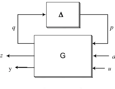
Consider the distributed parameter system, G, in ﬁgure 2.1. Let the signal d ∈ Rnd _{represent all distributed external inputs including disturbances, sensor noise, and}

commands, z ∈ Rnz _{represent the error signal,} _y ∈ _Rny _{be the measured variable,}

and u ∈ Rnu _{be the control input. Signals} _{p, q} ∈ _Rnp _{are pseudo input/output}

channels for uncertainty. Deﬁne the state vector x(s, t) = [xt xs]T that has both temporal and spatial components such that, xt_∈ _Rm₀ _{represent the temporal states} and xs _∈_Rm1+m−1+···+mL+m−L _{be the spatial states.}

G

z

y

q p

u y

d

Figure 2.1: Distributed parameter system

It is hard to ﬁnd exact solutions to the partial diﬀerential equations for spatially varying distributed systems. Therefore, approximated solutions are often sought through spatial discretization [29]. In this regard, the system is discretized in its spatial variable s = [s₁, s₂,· · · , sL]

T

. Then, deﬁne the spatial shift operator Si [10] as,

(23)

and will be used for the rest of the study. On the other hand, temporal states can be discretized as well. In that case, T becomes a temporal shift operator and is deﬁned in equation (2.7). In other words,

either Tx(s, t) := ∂x(s, t)

∂t (2.6)

or Tx(s, k) :=x(s, k+ 1) (2.7)

Then, deﬁnew(s, t) = [wt _ws_]T _{such that,} wt= ∆_Txt(s, t), ∆_T:=TIm0

ws= ∆_Sxs(s, t), ∆_S := diag(S₁Im1,S−11 Im−1,· · · ,SLImL,S

−1 L Im₋L)

The state-space realization of the systemG, which is indeed a group of subsystems, above takes the following form:

          wt ws q(s, t) e(s, t) y(s, t)           =          

Att _Ats _Bt

0 B1t B2t Ast _Ass _Bs

0 B1s B2s C₀t C₀s D₀₀ D₀₁ D₀₂ Ct

1 C1s D10 D11 D12 Ct

2 C2s D20 D21 D22

                    xt xs p(s, t) d(s, t) u(s, t)           (2.8)     xt xs p(s, t)    =    

∆−1_T ∆−1_S

∆(s)         wt ws q(s, t)     (2.9)

The integer variable s is indexed over all subsystems. The state space data is in linear fractional dependency [31] of the structured parameter ∆. Parameter δ describes the spatial variation of the distributed system and it is uniquely determined for any given variable s. ∆ obeys the following structure,

∆=∆ = diagδ₁Is₁,· · · , δgIsg

: δi :N→R,|δi| ≤1, i= 1,· · · , g

(24)

matrices are deﬁned,

A =

Att _Ats Ast _Ass

, B₀ =

Bt 0 Bs 0

, B₁ =

Bt 1 Bs 1

B2 =

Bt 2 Bs 2 , (2.10) C0 =

C₀t C₀s

C1 =

C₁t C₁s

, C2 =

C₂t C₂s

(2.11)

2.3 System Interconnection

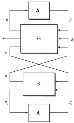
Given the distributed parameter system Gwith all the weighting functions included, we would like to ﬁnd a controller K which produces control signals u based on the measurement signals y such that the interconnection M = Fl(G,K) is well-posed and the closed loop system M is exponentially stable and the inducedL₂ norm from inputs d to outputs e is minimized.

We are interested in the distributed parameter-dependent controller K that has the same structure as the distributed plant G. In other words, the controller K also depends on the structured parameter ∆ in linear fractional form. Thus, state-space realization of the controller is given by,

      

w_kt ws k

qk(s, t) u(s, t)        =       

Att_k Ats_k Bt₀_,k B₁t_,k Ast

k Assk Bs0,k B1s,k C₀t_,k C₀s_,k D₀₀,k D01,k Ct

1,k C1s,k D10,k D11,k

             

xt_k xs k

pk(s, t) y(s, t)        (2.12)     xt k xs k

pk(s, t)

   =    

∆−1_T ∆−1_S

∆(s)         wt k ws k

qk(s, t)

  

 (2.13)

where xk = [xtk x s k]

T _∈

Rnk_, _p

(25)

q q q q q q - - - - -? 6 ? 6 ? 6 ? 6 - -G₀ K₀ G₁ K₁ Gs Ks

Gs+1

Ks+1 y₀ u₀ y₁ u₁ ys us ys+1 us+1

Figure 2.2: Distributed control architecture

If each controller Ks has only the local information ys, us and no interaction with its neighbors, then we have a completely decentralized control. Implementation of completely decentralized controllers is easier because only the local information needs to be processed. However, no computationally tractable algorithms exist for the de-sign of the completely decentralized controllers with performance and stability guar-antees. Therefore, in our distributed control approach, the interaction between the neighboring controllers exists, which leads us somewhere in between a completely decentralized and completely centralized control.

Deﬁne the controller K={Ak,Bk,Ck,Dk}as,

Ak =

Att k Atsk Ast

k Assk

, Bk=

Bt

0,k B1t,k Bs

0,k B1s,k

Ck =

Ct

0,k C0s,k Ct

1,k C1s,k

, Dk =

D₀₀,k D01,k D₁₀,k D11,k

Then, the closed-loop system M=Fl(G,K) shown in ﬁgure 2.3 can be written as,

       wt cl ws cl

qcl(s, t) z(s, t)        =    

Acl B0,cl B1,cl C0,cl D00,cl D01,cl C1,cl D10,cl D11,cl

           xt cl xs cl

(26)

G K w z u y q q p p_k k d

Figure 2.3: Closed-loop LFT Framework

    xt cl xs cl

pcl(s, t)

   =       

∆−1_T ∆−1_S

∆(s) ∆(s)            wt cl ws cl

qcl(s, t)

  

 (2.15)

where, xcl =

xt _xt

k xs xsk

T

, pcl =

p pk

T ,qcl =

q qk

T , and    

Acl B0,cl B1,cl C0,cl D00,cl D01,cl C1,cl D10,cl D11,cl

   =        Att

cl Atscl B0t,cl B1t,cl Ast_cl Ass_cl B₀s_,cl B₁s_,cl Ct

0,cl C0s,cl D00,cl D01,cl C₁t_,cl C₁s_,cl D₁₀,cl D11,cl

      

Clearly, the temporal and spatial state variables need to be grouped together. Therefore, a permutation matrix P is needed to convert the closed loop state-space data into the standard system deﬁnition. So, deﬁne,

P :=

Pt ₀ _Pt k 0 0 Ps ₀ _Ps

k

(27)

where Pt, Ps, P_kt and P_ks are permutation matrices compatible with associated tem-poral and spatial dimensions of the plant and the controller. Thus, the closed-loop system (2.14)-(2.15) can be related to the plant and controller data as,

Acl =PAcl¯ PT, (2.16)

B0,cl B1,cl

=P

¯

B0,cl B1¯,cl

(2.17) C0,cl C1,cl = ¯ C0,cl ¯ C1,cl

PT, (2.18)

D₀₀,cl D01,cl D₁₀,cl D11,cl

=

¯

D₀₀,cl D¯01,cl ¯

D₁₀,cl D¯11,cl

(2.19) where,     ¯

Acl _B0¯_,cl _B1¯_,cl ¯

C0,cl D¯₀₀,cl D¯₀₁,cl ¯

C1,cl D¯10,cl D¯11,cl

   =          

A 0 B0 0 B1

0 0 0 0 0

C0 0 D₀₀ 0 D₀₁

0 0 0 0 0

C1 0 D₁₀ 0 D₁₁

          +          

0 B₂ 0 I 0 0 0 D₀₂ 0

0 0 I

0 D₁₂ 0

          Ak Bk Ck Dk    

0 I 0 0 0

C2 0 D₂₀ 0 D₂₁

0 0 0 I 0

   

2.4 Stability and Performance Analysis

(28)

First, we deﬁne the block diagonal matrix set X and scaling matrix set D as, X :=X = diagXt, Xs : Xt =XtT >0, Xs =XsT (2.20) D:=D= diag{Ds1_,· · · _{, D}sg}_:_D₌_DT _>₀ _(2.21)

Yet, another matrix transformation is needed before the stability and performance conditions can be tested. All theorems presented in this chapter have been derived for distributed systems that are continuous both in temporal and spatial dimensions. Since the system M is discretized in spatial dimension, a bilinear transformation is required to obtain its continuous counterpart.

So, letH= diagIm₀,cl, Im1,cl, Im−1,cl,· · · , ImL,cl, Im−L,cl

, then, the transformation in spatial dimension can be obtained by

˜ xs ws =

H √2I √ 2H I ˜ ws xs (2.22)

Now, the continuous system’s state-space realization under such transformation is given by,

˜

Ass_cl =H(Ass_cl −I) (Ass_cl +I)−1, (2.23)

˜ Ast

cl B˜s0,cl B˜1s,cl

=√2H(Ass_cl +I)−1

Ast

cl B0s,cl B1s,cl

(2.24)     ˜ Ats cl ˜ Cs 0,cl ˜ C₁s_,cl

  

=√2

    Ats cl Cs 0,cl C₁s_,cl

  

(Asscl +I)−1 (2.25)

    ˜ Att

cl B˜0t,cl B˜1t,cl ˜

Ct

0,cl D˜00,cl D˜01,cl ˜

C₁t_,cl D˜₁₀,cl D˜11,cl

   =     Att

cl B0t,cl B1t,cl Ct

0,cl D00,cl D01,cl C₁t_,cl D₁₀,cl D11,cl

   −     Ats cl Cs 0,cl C₁s_,cl

  

(Ass_cl +I)−1

Ast

cl B0s,cl B1s,cl

(29)

Theorem 1 The distributed parameter-dependent system (2.14)-(2.15) is exponen-tially stable if there exists a symmetric matrixXcl ∈ X and a scaling matrix Lcl ∈ D, such that

I A˜T

cl 0 C˜0T,cl 0 B˜T₀_,cl I D˜T₀₀_,cl

      

0 Xcl Xcl 0

0

0 −Lcl 0 0 Lcl

              I 0 ˜ Acl _B˜

0,cl

0 I

˜

C0,cl D˜00,cl

       <0

Proof of theorem 1 can be found in [44]. A distributed Lyapunov function is used to ensure the stability. However, apart from the standard Lyapunov stability result for a single system, only the ﬁrst block Xt

cl of variable Xcl is required to be strictly positive in order to guarantee the stability of the distributed system.

Similarly, the performance of the distributed parameter-dependent system can be determined with the results provided by the next theorem. The proof of this theorem can also be found in [44].

Theorem 2 The distributed parameter-dependent system (2.14)-(2.15) is exponen-tially stable and has z2 < γd2 for all admissible uncertainties ∆ if there exists a symmetric matrix Xcl ∈ X and a scaling matrix Lcl ∈ D, such that

        T            

0 Xcl Xcl 0

0 0

0 −Lcl 0 0 Lcl

0

0 0 −γI 0

0 1_γI

                       

I 0 0

˜

Acl _B0˜_,cl _B1˜_,cl

0 I 0

˜

C0,cl D˜00,cl D˜01,cl

0 0 I

˜

C1,cl D˜10,cl D˜11,cl

(30)

us a simple way to derive LMI solutions from one system representation form to another.

2.5 Controller Synthesis

Consider the open-loop distributed parameter-dependent system G of (2.8)-(2.9). The control design objective is to minimize the induced L₂ norm from d toz, where the signal’s 2-norm is deﬁned in equation (2.3). Therefore in mathematical terms, we seek the distributed parameter-dependent controller (2.12)-(2.13) to minimizeγ such that

z2 ≤γd2

The main assumptions on the plant description are,

(A1) (A,B2,C2) is stabilizable and detectable by a distributed controller, (A2) D₂₂ = 0

The ﬁrst assumption guarantees the existence of a stabilizing distributed output-feedback controller. Assumption (A2) can be relaxed by redeﬁning the output variable [43].

Although theorem 2 provides us with the results to determine stability and the performance level of a distributed parameter-dependent system, it cannot be used for the design of a stabilizing controller K. Equation (2.27) is an LMI in terms of the decision variableXcl. However, the LMI must be partitioned compatibly to plant and controller statesn and nk such that,

Xcl =

Y N NT

, X_cl−1 =

X M

MT

(31)

Ass=H(Ass−I) (Ass+I)−1, (2.28)

Ast _Bs 0 B1s

=√2H(Ass+I)−1

Ast _Bs 0 B1s

(2.29)     Ats

C₀s

Cs 1   

=√2

   

Ats C₀s Cs 1

  

(Ass+I)−1 (2.30)

   

Att _Bt 0 Bt1

C₀t D₀₀ D₀₁

Ct

1 D10 D11

   =    

Att _Bt 0 B1t C₀t D₀₀ D₀₁ Ct

1 D10 D11

    −     Ats C₀s Cs 1

  

(Ass+I)−1

Ast B₀s Bs₁

(2.31)

For the simplicity of the theorem, group the matrices such that,

A=

Att _Ats

Ast _Ass

, B0 =

Bt 0 Bs 0

, B1 =

Bt 1 Bs 1 B2 = Bt 2 Bs 2 , C0 =

C₀t C₀s

C1 =

C₁t C₁s

, C2 =

C₂t C₂s

The alternative version of theorem 2 that leads to the solution of the output-feedback control synthesis problem is expressed in the following theorem.

(32)

that NT X         T             0 X

X 0 0 0

0 −L 0

0 L 0

0 0 −

1 γI 0 0 γI                        

−AT −CT

0 −C1T

I 0 0

−BT

0 −D00T −D10T

0 I 0

−BT

1 −D01T −D11T

0 0 I

           

NX >0

(2.32) NT Y         T             0 Y

Y 0 0 0

0 −J 0

0 J 0

0 0 −γI 0

0 1_γI

                       

I 0 0

A B0 B1

0 I 0

C0 D₀₀ D₀₁

0 0 I

C1 D₁₀ D₁₁

           

NY <0 (2.33)

Yt _I I Xt

≥0 (2.34)

L I I J

≥0 (2.35)

where

NX = Ker

BT

2 DT02 DT12

, NY = Ker

C2 D20 D₂₁

Theorem 3 is a generalization of LFT-type linear parameter varying control ap-proach [32] to spatially varying distributed systems. Synthesis conditions are in the form of LMIs, which are convex optimization problems. They can be solved eﬃciently using interior-point optimization algorithms [17], [30].

(33)

• I−XY must be non-singular so perturbXandY accordingly, if necessary. LetM NT ₌_I₋_XY _{and reconstruct} _X

cl such that

Xcl =

Y N

NT ₋_M−1_XN

• Next, compute the matricesF and G, which are deﬁned by,

F :=−

DT 02 D12T

L 0 0 1_γI

D₀₂ D₁₂ −1 BT

2X−1+

DT 02 DT12

L 0 0 1_γI

C0

C1

G :=−

Y−1C₂T +

B0 B1

L 0 0 γI

D₂₀T

DT 21

D₂₀ D₂₁ L −1 ₀ 0 _γ1I

DT₂₀

DT 21

−1

• Compute the state-space matrices of the controller

Ak =−N−1

AT ₊_Y _A₊_B

2F+GC2

X

+Y

B0 B1+G

D₂₀ D₂₁ L 0 0 _γ1I

BT 0 BT 1 + CT 0 C1T

L−1 0 0 1_γI

C0 C1 + D₀₂ D₁₂ F X

M−T (2.36)

Bk =N−1YG (2.37)

Ck =FXM−T (2.38)

Dk =0 (2.39)

(34)

Chapter 3 Modeling of Flexible Structure

In this chapter, the dynamic model of a non-uniform flexible structure is developed. A cantilever beam with a variable thickness is considered as the non-uniform flexible structure. Although analyzing the dynamics of the flexible beam is a well known problem, often the modal approach is used in modeling. Such an approach is not suitable for non-uniform beam due to the lack of analytical solution. On the other end, our interest is in model-based control. Therefore, a distributed state-space model of the non-uniform flexible beam is developed directly using the partial differential equation that governs the beam’s motion in transverse direction.

We will start with the derivation of the equation of motion of the non-uniform beam in transverse direction. Next, the modeling of the parameter variations is presented. In section 3.3, the resulting equation is discretized in the spatial dimension, which leads to the distributed state-space model described in section 3.4. Finally, the chapter will be concluded with the modal analysis and veriﬁcation of the developed distributed model.

3.1 Equation of Motion

(35)

one end to a solid base, and the other end is free to move in the transverse direction. Let v(x, t) represent the transverse displacement, f(x, t) be the distributed external forces including both the control forces u(x, t), and the disturbance forces d(x, t). It is assumed that the displacement can be measured and control forces can be applied at prespeciﬁed locations by distributed sensors and actuators placed on the surface of the beam. However, the dynamics of the beam is assumed to remain unchanged, despite the presence of these sensors and actuators.

x z

y

w_b

L t

t

b

t

f (x,t)

v (x,t)

Figure 3.1: Non-uniform ﬂexible cantilever beam

(36)

The partial diﬀerential equation of the transverse motion of the non-uniform ﬂex-ible beam is then expressed in undamped Bernoulli-Euler form as:

∂2 ∂x2

EI(x)∂

2_{v(x, t)} ∂x2

+ ∂ 2

∂t2 [ρ(x)v(x, t)] =f(x, t) (3.1) whereρ(x) is the mass per unit length and EI(x) is the ﬂexural rigidity of the beam. E is the Young’s modulus and I(x) is the area moment of inertia about z-axis.

For the cantilever beam case, the displacement and slope must be zero at the ﬁxed end, and the shear force and bending moment must be zero at the free end. Therefore, in mathematical terms these imply the following boundary conditions for equation (3.1):

v(x, t) = 0 x= 0 (3.2)

∂v(x, t)

∂x = 0 x= 0 (3.3)

∂ ∂x

EI(x)∂

2_v_{(x, t)} x2

= 0 x=L (3.4)

EI(x)∂

2_{v(x, t)}

x2 = 0 x=L (3.5)

It is assumed that the thickness of the beam changes linearly with xand the beam has a maximum thickness of tb at the fixed end. Next, we define the thickness ratio ct as the ratio of the thickness of the beam at the fixed end to thickness at the free one,

ct = tt tb

Thickness of the beam at any cross-section tc(x) is then formulated as: tc(x) = tb

1−(1−ct) x L

(3.6) The change in the thickness results in the spatial dependence of the parameters ρ(x) and I(x) to the variable x, which is the distance measured from the ﬁxed end. Assuming the beam has a rectangular cross-section these are expressed in the form:

ρ(x) =ρvwbtb

1−(1−ct) x L

(37)

I(x) = 1 12wbt

3 b

1−(1−ct) x L

3

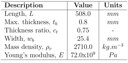
(3.8) where ρv is the mass density, wb is the width and L is the length of the beam. The ﬂexible beam used in this study is made of aluminum and its mechanical and geometric properties are given in table 3.1.

Table 3.1: Non-uniform ﬂexible beam parameters

Description Value Units

Length, L 508.0 mm

Max. thickness, tb 0.8 mm Thickness ratio, ct 0.75

-Width, wb 25.4 mm

Mass density, ρv 2710.0 kg.m−3 Young’s modulus, E 72.0x109 P a

Substituting equations (3.7) and (3.8) into (3.1), taking the partial derivatives, simplifying and rearranging the terms, the partial diﬀerential equation of motion of the non-uniform ﬂexible beam now becomes,

∂2v(x, t) ∂t2 =−

Et2_b ρv

(1−ct)2 2L2

∂2v(x, t) ∂x2 −

(1−ct) 2L

1−(1−ct) x L

_∂3_{v(x, t)} ∂x3 + 1

12

1−(1−ct) x L

₂ _∂4_{v(x, t)} ∂x4

+ d(x, t) +u(x, t) ρvwbtb

1−(1−ct)_Lx

(3.9)

3.2 Modeling the Structured Uncertainty

As mentioned in the previous chapter, the parameter dependence on the spatial vari-able x can be treated as parametric uncertainty. Let δ be the uncertain parameter deﬁned as follows,

δ = 2x

(38)

therefore |δ| ≤1 for all x∈[0, L]. Thus, equation (3.9) becomes ∂2v(x, t)

∂t2 =− Et2_b

ρv

(1−ct)2 2L2

∂2v(x, t) ∂x2 −

(1−ct)

4L (1 +ct−(1−ct)δ)

∂3v(x, t) ∂x3 + 1

48(1 +ct−(1−ct)δ)

2 ∂4v(x, t) ∂x4

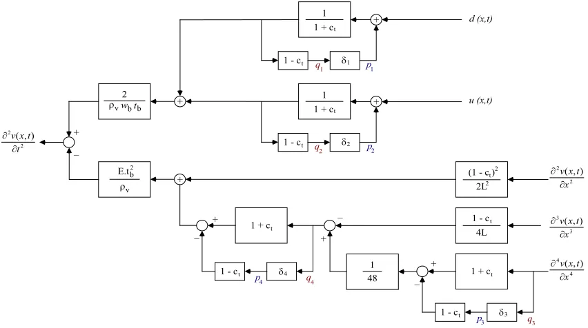
+ 2(d(x, t) +u(x, t)) ρvwbtb(1 +ct−(1−ct)δ)

(3.11) We would like to describe the spatial dependence of the parameters on x in a linear fractional form. The LFT structure can be obtained by a simple manipulation, which is often referred as ’pulling out the δ’s’ [48]. First, a simple block diagram of equation (3.11) is drawn. Then, pseudo inputs and outputs pi,qi are introduced for each δ and all the uncertainties are removed from the diagram.

U

E.t_b2

v

1 + ct

1 - ct ₄₈1 1 + ct

1 - ct

4L

(1 - c )t

2L

2 2

1 + ct

1 - ct

1

1 + ct

1 - ct

1 G2 G1 G3 G4 d (x,t) u (x,t) q₁ q₂ q₃ q₄ p₁ p₂ p₃ p₄

U_vw_btb

2 + + + + + _ _ _ _ + + + c2v(x,t)

c2t2 2₍_,₎

t t x v w w

c2v(x,t) cx2

c3v(x,t) cx3

c4v(x,t) cx44

4 ₍_,₎

x t x v w w 3 3 ₍_,₎

x t x v w w 2 2 ₍_,₎

x t x v w w

Figure 3.2: Block diagram representation of equation (3.11)

(39)

q₁ = 1 1 +ct

d(x, t) + 1−ct 1 +ct

p₁ (3.12)

q₂ = 1 1 +ct

u(x, t) + 1−ct 1 +ct

p₂ (3.13)

q₃ = ∂

4_{v(x, t)}

∂x4 (3.14)

q₄ = 1 +ct 48

∂4v(x, t) ∂x4 −

1−ct 4L

∂3v(x, t) ∂x3 −

1−ct

48 p3 (3.15)

3.3 Spatial Discretization

Structural elements like beams are continuous systems, and the exact solutions to the partial differential equations of their motion cannot be found except for some special cases. Hence, approximate solutions are often sought through spatial discretization. In this study, partial derivatives in spatial dimension are approximated with the central finite difference scheme, using N grid points separated by a length of h on the beam. Therefore, continuous flexible beam is discretized into (N−1) subsystems (i.e. L= (N−1)h). However, in the spatial discretization, while the number of grids may vary, the locations of the displacement measurements and of the applied control forces are kept fixed.

∂2v(x, t) ∂t2 =−

Et2_b ρv

(1−ct)2

2L2h2 (v(x−h, t)−2v(x, t) +v(x+h, t)) −(1−c2t)

8Lh3 (−v(x−2h, t) + 2v(x−h, t)−2v(x+h, t) +v(x+ 2h, t)) +(1 +ct)

2

48h4 (v(x−2h, t)−4v(x−h, t) + 6v(x, t)−4v(x+h, t) +v(x+ 2h, t))] + 2(1−ct)

ρvwbtb(1 +ct)

(p₁+p₂) + Et 2

b(1−ct) ρv

(1 +ct)

48 p3 +p4

+ 2

ρvwbtb(1 +ct)

(d(x, t) +u(x, t)) (3.16)

(40)

non-uniform ﬂexible beam takes its ﬁnal form to be used in state-space model by replacing the continuous spatial variable x with its discrete counterpart s,

T2v(s, t) = −Et 2 b ρv

(1−ct)2 2L2h2

S−1+S−2 − (1−c 2 t) 8Lh3

−S−2+ 2S−1 −2S+S2

+(1 +ct) 2

48h4

S−2−4S−1−4S+S2+ 6 v(s, t) + 2(1−ct) ρvwbtb(1 +ct)

(p₁+p₂) +Et

2

b(1−ct) ρv

(1 +ct)

48 p3 +p4

+ 2 (d(s, t) +u(s, t)) ρvwbtb(1 +ct)

(3.17) Finite diﬀerence approximation of the spatial derivatives are also applied to the boundary conditions at both ends. They will be used in the MATLAB simulation code.

At the ﬁxed end,

v(x, t)|x₌₀= 0 ⇒ v(s, t) = 0, s= 1 ∂v(x, t) ∂x !! !! ! x=0

= 0 ⇒ v(s−1, t) =v(s+ 1, t), s= 1

At the free end,

EI(x)∂

2_{v(x, t)} x2

!! !! !

x=L

= 0 ⇒ v(s+ 1, t) = 2v(s, t)−v(s−1, t), s =N ∂

∂x

EI(x)∂

2_{v(x, t)} x2

!! !! !

x=L

= 0 ⇒ v(s+ 2, t) = 4v(s, t)−4v(s−1, t)

+v(s−2, t), s =N

3.4 State-Space Model

(41)

displacements of the neighboring nodes. In this regard,

xt=

v(s, t) Tv(s, t)

, xs=

      

S−2v(s, t) S−1v(s, t) S2v(s, t) S v(s, t)

       (3.18)

The external inputs to the system are noise n(s, t) in the displacement measure-ments, distributed disturbance forcesd(s, t) and the distributed actuator forcesu(s, t). Next, the system outputs are deﬁned as the error signalsz(s, t) and displacement mea-surementsy(s, t). The error signals are chosen to penalize the control input asz₁(s, t) and the node displacement asz₂(s, t).

Then, state-space formulation of the distributed model of the non-uniform ﬂexible beam becomes,

wt _ws _{q z}

1 z2 y

T =

A B

C D x

t _xs _{p n d u}

T (3.19) where     xt xs p    =       

T−1I₂ SI₂

S−1I₂ δI₄            wt ws q(s, t)     and A=            

0 1 0 0 0 0

a₂₁ 0 a₂₃ a₂₄ a₂₅ a₂₆

0 0 0 1 0 0

1 0 0 0 0 0

0 0 0 0 0 1

1 0 0 0 0 0

           

, B =

           

0 0 0 0 0 0 0

b₂₁ b₂₂ b₂₃ b₂₄ 0 b₂₆ b₂₇

0 0 0 0 0 0 0

(42)

C =               

0 0 0 0 0 0

c₃₁ 0 c₃₃ c₃₄ c₃₅ c₃₆ c₄₁ 0 c₄₃ c₄₄ c₄₅ c₄₆

0 0 0 0 0 0

1 0 0 0 0 0

              

, D =

              

d₁₁ 0 0 0 0 d₁₆ 0 0 d₂₂ 0 0 0 0 d₂₇

0 0 0 0 0 0 0

0 0 d₄₃ 0 0 0 0

0 0 0 0 0 0 1

0 0 0 0 0 0 0

0 0 0 0 1 0 0

              

where non-zero coeﬃcients are deﬁned by: a₂₁= Et

2 b ρv

(1−ct)2 L2h2 −

(1 +ct)2 8h4

a₂₃=−Et 2 b 8ρv

(1−c2_t) Lh3 +

(1 +ct)2 6h4

a₂₄= Et 2 b 2ρv

−(1−ct)2 L2h2 +

(1−c2_t) 2Lh3 +

(1 +ct)2 6h4

a₂₅= Et 2 b 8ρv

(1−c2_t) Lh3 −

(1 +ct)2 6h4

a₂₆=−Et 2 b 2ρv

(1−ct)2 L2h2 +

(1−c2_t) 2Lh3 −

(1 +ct)2 6h4

b₂₁=b₂₂ = 2(1−ct) ρvwbtb(1 +ct) b₂₃= Et

2

b(1−c2t) 48ρv b₂₄= Et

2

b(1−ct) ρv

b₂₆=b₂₇ = 2 ρvwbtb(1 +ct) c₃₁= 6

h4 c33 =c35= 1

h4 c34 =c36=− 4 h4 c₄₁= (1 +ct)

8h4 c₄₃= (1 +ct)

48h4 +

(43)

c₄₄ =−(1 +ct) 12h4 −

(1−ct) 4Lh3 c₄₅ = (1 +ct)

48h4 −

(1−ct) 8Lh3 c₄₆ =−(1 +ct)

12h4 +

(1−ct) 4Lh3 d₁₁ =d₂₂= (1−ct)

(1 +ct) d₁₆ =d₂₇= 1

(1 +ct) d₄₃ =−(1−ct)

48

3.5 Modal Analysis and Beam Model Validation

So far, the state-space formulation of the non-uniform ﬂexible beam has been devel-oped based on the governing partial diﬀerential equation of motion. Before proceeding further with the controller design, validity of the developed distributed model will be discussed in this section.

Note that the developed model is only an approximation of the dynamics of the actual system because of the spatial discretization. It is necessary to know how many grid points are suﬃcient in order to capture the beam dynamics accurately. Therefore, a comparison study between the exact solution and the developed distributed model is needed.

Unfortunately, the exact solution to the equation of motion of a non-uniform ﬂexible beam is not available. Then, another approximate solution, which is known to give an accurate description of the actual system, must be used for comparison purposes. Therefore, a ﬁnite element model of the non-uniform beam will be compared with the distributed model.

(44)

Uniform Beam Case

First, a uniform flexible cantilever beam is considered. Various finite element models were built in ANSYS using different number of 2D rectangular elements, and the first five natural frequencies with their corresponding mode shapes were extracted. The resulting natural frequencies are given in table 3.2 along with the exact ones [23]. It is clearly seen that as the number of elements in FEM increases, the approximated natural frequencies converges to the actual ones, from above.

Table 3.2: First ﬁve natural frequencies of a uniform ﬂexible beam

Method ω₁ (rad/s) ω₂ (rad/s) ω₃ (rad/s) ω₄ (rad/s) ω₅ (rad/s) FEM, 100-Element 16.443 101.914 284.997 558.648 924.205 FEM, 500-Element 16.443 101.890 284.804 557.887 922.094 FEM, 1000-Element 16.443 101.889 284.798 557.863 922.028 FEM, 5000-Element 16.441 101.889 284.796 557.856 922.007 Analytical 16.218 101.638 284.589 557.682 922.075

In the distributed model case, by concatenating the distributed model into a single lumped model, one can calculate the natural frequencies of the given uniform beam. If the subsystems are modeled correctly, those should also converge to the exact values qradually. This will be demonstrated from the simulation plots later on.

(45)

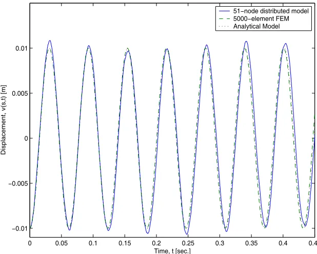
larger. It is observed that as the number of nodes along the beam length increases, the amount of this error decreases and finally converges to the analytical solution. It is also seen that the second and third mode responses from finite element model is inferior to the distributed model solutions even for large number of finite elements are used.

0 0.2 0.4 0.6 0.8 1 1.2 1.4 1.6 1.8 2

−0.01

−0.005 0 0.005 0.01

Time, t [sec.]

Displacement, v(s,t) [m]

51−node distributed model 5000−element FEM Analytical Model

Figure 3.3: Deﬂection of the free end of the uniform beam, 1st _{mode excited}

Another set of initial conditions is tested to get a combined mode response of the uniform beam. In this study, it is assumed that the uniform beam is initially deflected by a point force applied at the free end to give a tip deflection of 0.01m. The response of the flexible beam to this set of initial conditions is plotted in figure 3.6. Again, both approximate solutions are very close to the analytical solution.

(46)

0 0.05 0.1 0.15 0.2 0.25 0.3 0.35 0.4 0.45

−0.01

−0.005 0 0.005 0.01

Time, t [sec.]

Displacement, v(s,t) [m]

51−node distributed model 5000−element FEM Analytical Model

Figure 3.4: Deﬂection of the free end of the uniform beam, 2nd _{mode excited}

uniform flexible beam accurately while using considerably less number of states. Fur-thermore, finite element model and distributed model converge to the actual system from opposite sides, i.e., finite element model always predicts the frequency of vibra-tion slightly higher while the frequency of the distributed model is slightly smaller than the actual one.

Non-uniform Beam Case