2D Position Detection of an Object Using Accelerometer Data

(1)

2D Position Detection of an Object Using

Accelerometer Data

Parmar Durvisha M

B.E. Student, Department of Electronics Engineering, Birla Vishwakarma Mahavidyalaya, Vallabhvidhyanagar, Anand,

Gujarat, India

ABSTRACT:This paper describes different methods used for interpreting the accelerometer data to find 2D co-ordinates of an object based not numerical integration. In the present era, positioning based on different inertial sensors and electromechanical devices has become extremely important because of the introduction of MEMS. These kinds of devices are mounted inside phones or PDAs and provide the current location of an object based on the acceleration information. But these kinds of inertial sensors have the limitation in that a small error in the acceleration information can result into a large variation in the position as the acceleration data is double integrated to obtain the displacement. But to overcome the limitations of such sensors a positioning algorithm is developed to provide the displacement information from the acceleration information obtained from an accelerometer. The primary focus of this document is to describe different methods to obtain the location of an object using the acceleration information obtained from the accelerometer.

KEYWORDS: Position detection; accelerometer data; double integration with filter; Kalman filter; sensors for position detection; accelerometer for position detection.

I.INTRODUCTION

In the present fast-growing technological market, there are many products available for determining the position of an object. These smart devices are mounted on a PDA or a GPS system to provide the exact co-ordinates of an object. Accelerometer is one such device with the help of which we can obtain a 2D and 3D position of an object based on the acceleration information obtained. Accelerometer is an electro-mechanical device which provides the acceleration of an object at any given time. So we cannot directly get the position information of an object from the accelerometer data.

By definition the rate of change of velocity of an object is known as acceleration and the rate of change of velocity of an object is known as placement. So putting these terms in to a

equation[6], we have

⃗= ⃗and ⃗= ⃗

(2)

ISSN(Online): 2320-9801

ISSN (Print) : 2320-9798

I

nternational

J

ournal of

I

nnovative

R

esearch in

C

omputer

and

C

ommunication

E

ngineering

(A High Impact Factor, Monthly, Peer Reviewed Journal)

Website: www.ijircce.com

Vol. 6, Issue 12, December 2018

Therefore, =

So the entire document is organized as follows.

1. Problem definition and analysis.

2. List of probable errors.

3. Different solutions to overcome such errors.

4. Conclusion and future work.

II. .PROBLEM DEFINITION AND ANALYSIS

So as discussed earlier, the primary focus of this document is going to be on describing various methods of interpreting the accelerometer data to provide the position of an object. One such method which serves this purpose is numerical integration of the acceleration function over time. So once we have the acceleration function, we can double integrate it to get the displacement information of an object. So in the next paragraph, I will briefly describe the process of numerical integration.

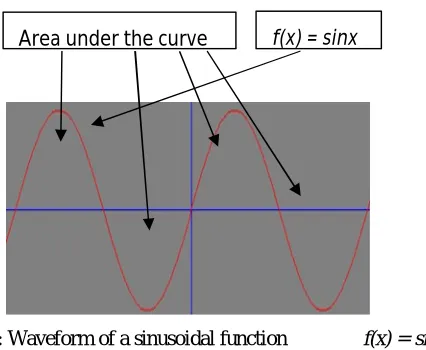
Basically, integration is used to find the area under a curve. Let’s say we have a sinusoidal function f(x) = sinxthen the

area that is bounded by the curve and the x-axis can be found out using integration. Figure 1 below shows a sinusoidal function f(x) = sinx.

Figure 1: Waveform of a sinusoidal function f(x) = sinx.

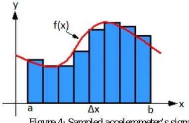
Now to find the area of the above curve between any two points we can use numerical integration. There are few different methods to perform numerical integration on a function but we will be describing only two methods here. One is the rectangular method and the other on is the trapezoidal method.

(3)

Figure 2: Rectangular integration Figure 3: Trapezoidal integration

Figure 2 and figure 3 shows the implementation of the two integration methods viz. rectangular and trapezoidal integration. The rectangular integration method samples the waveform at regular intervals with a rectangular pulse and the area under the curve is obtained by summing the area of all the rectangles. Similarly, for the trapezoidal method, a trapezoid is used to sample the signal and the area under the curve is obtained by the area of all the trapezoids. From the above figures (fig.2 & fig. 3) it is also evident that there are certain regions which are not covered by the sampling signal in both the rectangular and the trapezoidal methods. This is generally regarded as an error and it can be removed if we increase the number of samples used to sample a given function which is also considered as its sampling rate. But again increasing the sampling rate also has its drawback wherein it would be really difficult to filter the signal. As with the sinusoidal signal similarly, the acceleration signal obtained from the accelerometer can also be digitally integrated to obtain the area under the acceleration signal. Figure 4[6] shows the accelerometer signal and its integration using rectangular integration.

Figure 4: Sampled accelerometer’s signal

Representing the above in form of an equation, we have

∫ ( ) = lim → ∑ ( )∆

(4)

ISSN(Online): 2320-9801

ISSN (Print) : 2320-9798

I

nternational

J

ournal of

I

nnovative

R

esearch in

C

omputer

and

C

ommunication

E

ngineering

Figure 5: sampling error

From the above figure it is evident that the sampling signals are only able to give the instant values of the magnitude and hence the small areas under the curve which are not sampled result in what is know as the sampling error or the area error. A more better approach is to use the trapezoidal Integration as shown in figure 3 from which we can observe that the area error or the sampling error is much less compared to the rectangular method of integration.

Now in the next section, I will describe the process of double integration applied on the accelerometer signal. After that I will also provide information related to the noise involved and the filtering used to remove that noise signal.

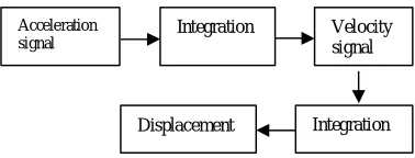
III. DOUBLE INTEGRATION

Below figure represents a block diagram for the double integration process[1].

Figure 6: Block diagram for double integration Now below are some figures showing the simulated waveforms representing an acceleration signal [7] for a double integrated sinusoidal signal. As is evident from the waveforms below, double integration of a sine wave results in another sine wave but with a change in the sign. So we see in the figure that the final sine wave is 180 degree out of phase from the original sine wave.

Acceleration signal

Displacement Integration

Velocity

signal

Integration

(5)

Figure 7: acceleration, velocity and displacement waveforms obtained after double integration[7]

Once the acceleration signal is integrated, it is likely to have a DC component [double integration].This DC component can be removed by using a high-pass filter. In the same manner the DC component resulting from the velocity signal can again be removed by passing it through another high-pass filter. The diagram below shows an improved block diagram for the double integration process including high-pass filters[1]

Figure 8: Block diagram for double integration with filter implementation[1].

Following are the simulation logs that are obtained by implementing filtering at each step in the double integration. .

Acceleration

signal Integration

High-pass filter

Velocity

signal

(6)

ISSN(Online): 2320-9801

ISSN (Print) : 2320-9798

I

nternational

J

ournal of

I

nnovative

R

esearch in

C

omputer

and

C

ommunication

E

ngineering

Figure 9: acceleration, velocity and displacement waveforms obtained after double integration[7] implementing filtering.

In addition to the advantages of using a filter, there also few disadvantages caused due to the transient response from the filter. There are various filters available that can be used for the double integration process to remove the DC component but here we will only discuss the Kalman Filter.

So far from the discussion we had on te double integration and the techniques used for implementing double integration viz. the trapezoidal and the rectangular method, it turns out that the trapezoidal method is a better approach for implementing the double integration method. Also we saw from the simulation waveforms that the rectangular method introduces area error in which some parts of the signal are not actually sampled by the sampling pulse. In comparison with the rectangular method for double integration, the trapezoidal method is a better approach. Again from the simulation data that was presented earlier in this paper it is evident that the trapezoidal method is a better approach then the rectangular method as it introduces a far lesser area error problem than the rectangular method.

IV.KALMAN FILTER

In almost many of the engineering systems or application involving interpretation and simulation of signals there has to be a filtering algorithm. For example, in a communication system the signal transmitted by the transmitter through a communication channel is bound to get corrupted before it reaches the intended receiver. This results in a noisy signal which needs to be filtered to ensure proper decoding of the received signal. Even in a regular power supply a signal might get corrupted by different components on the board and a good filter is required to give proper voltage and current values as required.

(7)

V. SIMULATION AND WAVEFROMS

So far we have discussed on how to interpret the acceleration signal obtained form the accelerometer and also discussed that we can use double integration methods to obtain the actual displacement of an object from the

acceleration signal. In the figures below, we have plotted few waveforms which demonstrates the

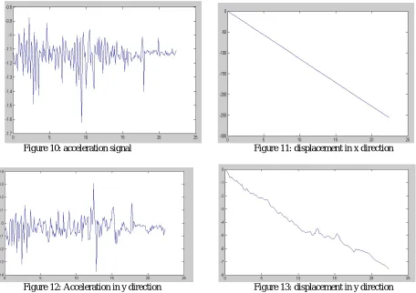
displacement of the object in 2D viz. the direction and the y-direction. Figure [10] is the acceleration signal obtained from the accelerometer. Figure [11] is the displacement obtained from the acceleration signal in the direction and figure [12] is the displacement obtained in the y-direction.

Figure 10: acceleration signal Figure 11: displacement in x direction

Figure 12: Acceleration in y direction Figure 13: displacement in y direction

(8)

ISSN(Online): 2320-9801

ISSN (Print) : 2320-9798

I

nternational

J

ournal of

I

nnovative

R

esearch in

C

omputer

and

C

ommunication

E

ngineering

Also, future work can be carried out to implement such position detection techniques in navigational and GPS systems with more accuracy.

VII. CONCLUSION

After working on all the above topics related to 2D position detection of an object with the use of an Accelerometer, it can be concluded that accelerometer gives promising results for knowing the displacement and the position of an object in 2D systems. The acceleration signal obtained from the accelerometer still needs to undergo the process of double integration where in the signal is integrated twice to get the actual displacement of the object.

It was also clear from the waveforms and the results that the at each stage of integration a good filtering algorithm is required. There are various filtering algorithms and tools available that can serve this purpose but for our case we just focused on Kalman filtering which proves to be a good filtering algorithm. Also, while talking of integration, of the two-integration process described in this paper viz. Rectangular method and Trapezoidal method it was quite obvious from the results that trapezoidal method is a good candidate for solving the area error which was more prevalent in the rectangular method of integration. Finally, there is still a lot to be explored in this field for getting a good approximation or rather the actual position of an object in 2D and 3d using the accelerometers.

REFERENCES

[1] Hunter B. Gilbert, OzkanCelik& Marcia K.O’Malley,”Long-TermDouble Integration of acceleration for Position Sensing and Frequency

Domain System Identification”, July 2010, IEEE/ASME international Conference on Advanced Intellegent Mechatronics.

[2] AntonioFilieri&RossellaMelchiotti,”Position Recoveryfrom Accelerometer Sensors”

[3] Sebastijan Sprager&DamjanZazula,”Impact of Different Walking Surfaces on Gait Identification Based on Higher-Order Statistics of

Acceleromeeter Data ”, 2011 IEEE International Conference on Signal and Image Processing Appliocations.

[4] Greg Welch & Gary Bishop,”An Introduction to the Kalman FIlter”, Univeristy of North Carolina at Chapel Hill.

[5] Dan Simon,”Kalman Filtering”.

[6] Kurt SeifertandOscar Camacho,”Implementing Positioning Algorithms Using Accelerometers”, Rev Freescale Semiconductors.

[7] Lance D Slifka,”An Accelerometer Based Approach to Measuring Displacement of a Vehicle Body”.

[8] Rong, Taiping; Shen, Chenghu; Yuan, Zhongping; Xu, Songmei; Principle of Measureing the Displacement with Accelerometer and the Error