Study of model predictive control for path-following autonomous ground vehicle control under crosswind effect

(1)

Research Article

Study of Model Predictive Control for Path-Following

Autonomous Ground Vehicle Control under Crosswind Effect

Fitri Yakub,

1

Aminudin Abu,

1

Shamsul Sarip,

2

and Yasuchika Mori

3

1_{Malaysia Japan International Institute of Technology, Universiti Teknologi Malaysia, Jalan Semarak, 54100 Kuala Lumpur, Malaysia} 2_{UTM Razak School of Engineering and Advanced Technology, Universiti Teknologi Malaysia, Jalan Semarak,}

54100 Kuala Lumpur, Malaysia

3_{Graduate School of System Design, Tokyo Metropolitan University, 6-6 Asahigaoka, Hino, Tokyo 191-0065, Japan} Correspondence should be addressed to Fitri Yakub; [email protected]

Received 4 November 2015; Revised 1 March 2016; Accepted 17 March 2016 Academic Editor: Yongji Wang

Copyright © 2016 Fitri Yakub et al. This is an open access article distributed under the Creative Commons Attribution License, which permits unrestricted use, distribution, and reproduction in any medium, provided the original work is properly cited. We present a comparative study of model predictive control approaches of two-wheel steering, four-wheel steering, and a combi-nation of two-wheel steering with direct yaw moment control manoeuvres for path-following control in autonomous car vehicle dynamics systems. Single-track mode, based on a linearized vehicle and tire model, is used. Based on a given trajectory, we drove the vehicle at low and high forward speeds and on low and high road friction surfaces for a double-lane change scenario in order to follow the desired trajectory as close as possible while rejecting the effects of wind gusts. We compared the controller based on both simple and complex bicycle models without and with the roll vehicle dynamics for different types of model predictive control manoeuvres. The simulation result showed that the model predictive control gave a better performance in terms of robustness for both forward speeds and road surface variation in autonomous path-following control. It also demonstrated that model predictive control is useful to maintain vehicle stability along the desired path and has an ability to eliminate the crosswind effect.

1. Introduction

Today, model predictive control (MPC) is one of the more popular optimal control techniques which is widely employed for the control of constrained linear or nonlinear systems. MPC uses a mathematical dynamics process model to predict the future behaviour of the system and optimize the process control performance over a prediction horizon [1]. The MPC model can be used easily at different levels of the process control structure, such as multiple input and multiple output dynamics systems that offer attractive solutions for regulation and tracking problems, while guaranteeing stability [2]. Since the end of the 1980s, robust MPCs which explicitly take account of model uncertainties, constraints, and faults in the control actuator, plant-model mismatch, and disturbances or noise have been studied for more practical applications [3]. Numerous research studies have investigated the stability properties of MPC for systems without uncertainty and for uncertain linear systems. Several robust predictive formula-tions utilize the min–max approach, where the manipulated

input trajectory is computed by solving an optimization problem that requires minimizing the objective function and satisfying the input and state constraints over all possible real-izations of the uncertainty. These have been applied mainly to impulse response models and state-space approaches by solving a finite horizon open-loop control optimization prob-lem [4]. Due to its advantages, MPC has been impprob-lemented in several applications for automotive and other transportation active safety systems, such as active steering, active traction, active braking, and active differentials or suspension systems, in order to coordinate and improve vehicle handling, stability, and ride comfort [5–8].

A vehicle capable of handling many things at once, without any human intervention, can be termed as an auto-nomous vehicle. Basic functions of autoauto-nomous braking and steering however are insufficient; the vehicle has to have the ability to sense its surrounding plus being able to determine desired location, which can be achieved using a variety of instruments and pieces of equipment such as radar, global positioning system, on-board camera for vision, and

(2)

an independent operating unit. All sensory data are then computed for obstacle identification; avoidance is then exe-cuted using advanced control system. In this paper, we limit autonomous vehicles to ground vehicles, which are increas-ingly being studied by several researchers from academia, industry, and military. Several control methods are being used, including fuzzy logic [9], hybrid control [10], H-infinity control [11], and linear quadratic regulators [12]. The best comparative studies on model predictive control strategies for autonomous guidance vehicles can be found in Park et al. [13], Yoon et al. [14], and Falcone et al. [15], where a nonlinear dynamics model of a vehicle is used for the controller design of an active front steering manoeuvre in a double-lane change scenario. Keviczky et al. [16] studied the effect of side wind via an active front steering manoeuvre for an autonomous vehicle using nonlinear MPC. Since nonlinear MPC poses consid-erable challenges due to its real-time implementation algo-rithm, many researchers opted for linear MPC for their study. The assumption of this study are as follows: vehicle trajec-tory is known, as per Borrelli et al.’s [17] study, and the cross-wind effect will be assigned as a step response, since the crosswind effect disturbance on the vehicle can be approx-imated as a constant. In this paper, we extend the concept of MPC for application in vehicle manoeuvring problems where a trajectory optimization is solved at each time step. The trajectory was designed to be a double-lane changing sce-nario. The autonomous vehicle manoeuvring was simulated in a variety of conditions: low (10 ms−1) and high (30 ms−1) forward speed and low (icy) and high (concrete, wet) road friction surface with the intention of following predeter-mined trajectory as close as possible while maintaining vehicle stability. The control inputs were front steering angle, rear steering angle, and direct yaw moment control, while the output controls were the yaw angle and lateral vehicle posi-tion. Two different controllers were compared to evaluate the performance of the six-degree-of-freedom (6DoF) vehi-cle model: a simple (2DoF) controller without vehivehi-cle roll dynamic and a complex (3DoF) bicycle model controller with roll dynamics. Other performance indexes evaluated were efficacy and robustness of the MPC for the autonomous vehicle in terms of control and stability.

The main objective of this paper is to evaluate the robust-ness of model predictive control approaches for autonomous path-following car dynamics control with simple and com-plex models of the vehicle, while rejecting the effects of wind gusts to the system. There are many studies to be consulted in stabilization of the vehicle; examples are two-wheel steering (2WS) [15, 18], four-wheel steering (4WS) [19], and 2WS with direct yaw moment control (DYC) [5, 20, 21] with different control strategies. The first contribution of this paper is the effect of vehicle roll dynamics motion consideration to the system, whereas most previous papers only focused on a 2DoF vehicle model (lateral and yaw motion). Moreover, based on the authors’ knowledge, there is no comparative study for autonomous path-following vehicle control using MPC techniques for three control signal manoeuvres (includ-ing the three control signals here); the robustness evaluation discussed here becomes the main novelty of this paper. Furthermore, we would like to investigate the effectiveness

of model predictive control manoeuvres in the case of the crosswind effect to the system in a variety of forward speeds and road adhesions. The rest of the paper is organized as follows: Section 2 describes the linear vehicle model, linear tire model, and wind model. Next, a linear model predictive control algorithm concept is explained in Section 3. Section 4 examines and describes the effectiveness of the linear MPC for a car dynamics system on a two-lane change scenario. Lastly, conclusions and future works are given in Section 5.

2. Vehicle Model

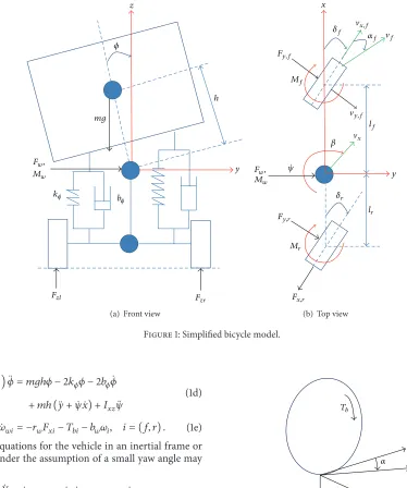
2.1. Bicycle Model. Figure 1 shows a well-known vehicle model, which is a single-track model based on the simplifica-tion that the right and left wheels are lumped in a single wheel at the front and rear axles. The simplified vehicle model used in this paper illustrates the motion movement and dynamics concerning the car vehicle subject to the longitudinal, lateral, yaw, roll, and rotational dynamics of the front and rear wheel motion, represented as 6DoF. The longitudinal, lateral, and yaw dynamics effects are shown in Figure 1(b) as a top view of the car vehicle, and in Figure 1(a), the roll dynamics effect is explained with the nomenclature for a front view of the vehicle. In this paper, the nonlinear vehicle was linearized based on the assumption that sin𝜃 = 0and cos𝜃 = 1for both steering angles, the vehicle side slip angle, and the roll angle. We also assumed that the whole vehicle mass is sprung, which is ignoring the suspension and wheel weights for unsprung mass. This linearized model still behaves and represents the actual nonlinear vehicle model at certain operating points of the region. The details of the mathematical calculation for the vehicle model are presented in Chen and Peng [22] for further knowledge.

In this paper, we use the following nomenclature: 𝐹_𝑥 and 𝐹_𝑦 represent the longitudinal and lateral tire forces, respectively, 𝐹_𝑧 is the normal tire load, 𝐹_𝑤 and 𝑀_𝑤 rep-resent the force and moment exerted by the side wind, respectively,𝑥,𝑦, and𝑧correspond to the coordinates of the body frame of a car position,𝑙is the vehicle wheelbase,𝑇_𝑏is the wheel torque,V_𝑥 andV_𝑦 are the longitudinal and lateral wheels velocities, respectively,𝛿_𝑓and𝛿_𝑟express the steering angle of the front and rear wheels, respectively,𝑀_𝑓and𝑀_𝑟 represent the reaction yaw moment appearing at the front and rear wheels, respectively,𝑀_𝑧is the total reaction of yaw moment of the wheels produced by the DYC,𝜇acts as the track friction coefficient,𝜓is the yaw/heading angle and ̇𝜓is the yaw rate,𝛽is the vehicle side slip angle, and𝜙and ̇𝜙are the roll and roll rate angles, respectively. The variable at the front and rear wheels is denoted by lower subscripts(⋅)_𝑓and(⋅)_𝑟.

The motion of longitudinal, lateral, yaw, roll, and rota-tional dynamics of the front and rear wheels using a 6DoF system based on a linear vehicle model is described through the following differential equations [23]:

𝑚 ̈𝑥 = 𝑚 ̇𝑦 ̇𝜓 + 2𝐹_𝑥𝑓+ 2𝐹_𝑥𝑟− 2ℎ𝑚 ̇𝜓 ̇𝜙 (1a)

𝑚 ̈𝑦 = −𝑚 ̇𝑥 ̇𝜓 + 2𝐹𝑦𝑓+ 2𝐹𝑦𝑟+ ℎ𝑚 ̈𝜙 + 𝐹𝑤 (1b)

𝐼_𝑧𝑧 ̈𝜓 = 2𝑙𝑓𝐹𝑦𝑓− 2𝑙𝑟𝐹𝑦𝑓+ 𝐼𝑥𝑧 ̈𝜙 + 𝑀𝑓+ 𝑀𝑟

(3)

z

h

y 𝜙

mg

Mw

b𝜙

Fzl F_zr

k𝜙

Fw,

(a) Front view

x

Fy,f

𝛿f x,f_𝛼 f f

Mf

y,f

lf

x

𝛽

Fw,

Mw

lr

𝛿r

Fy,r

Mr

Fx,r

̇

𝜓 _y

(b) Top view

Figure 1: Simplified bicycle model.

(𝐼_𝑥𝑥+ 𝑚ℎ2) ̈𝜙 = 𝑚𝑔ℎ𝜙 − 2𝑘_𝜙𝜙 − 2𝑏_𝜙 ̇𝜙

+ 𝑚ℎ ( ̈𝑦 + ̇𝜓 ̇𝑥) + 𝐼_𝑥𝑧 ̈𝜓 (1d)

𝐽_𝑏 ̇𝜔𝑤𝑖= −𝑟𝑤𝐹𝑥𝑖− 𝑇𝑏𝑖− 𝑏𝑤𝜔𝑖, 𝑖 = (𝑓 , 𝑟) . (1e)

The motion equations for the vehicle in an inertial frame or on𝑦-𝑥axis under the assumption of a small yaw angle may be given as

̇𝑋 = ̇𝑥cos𝜓 − ̇𝑦sin𝜓 =V_𝑥− ̇𝑦𝜓,

̇𝑌 = ̇𝑥sin𝜓 + ̇𝑦cos𝜓 =V_𝑥𝜓 + ̇𝑦.

(2)

2.2. Tire Model. Tire dynamics must be considered for the vehicle model, since the tires are the only contact that the vehicle has with the road surface. Besides the forces of gravity and aerodynamics, all the forces are induced by the tires, which may affect the vehicle chassis, handling, and stability. Their complexity and nonlinear behaviour must also reflect the operating condition of the controller over their whole region throughout varied manoeuvring range in long-itudinal, lateral, and roll directions. The most frequently used existing nonlinear tire models of application and structure are determined through key parameters and analytical con-siderations based on tire measurement data. They are called semiempirical tire models or Pacejka tire model [24].

On the other hand, the nonlinear tire model can also be described linearly for some parts of the operating con-ditions; therefore in this paper, we will consider the linear

Fx

x

Fy

𝛼

Fz

Tb

Figure 2: Tire model.

tire model. Figure 2 illustrates the terminology used for describing the longitudinal, lateral, and vertical tire forces and their orientation. Thus, the linear tire model is valid under constant normal load forces on the tires, constant longitudinal slip of tires, and neglected aerodynamic drag. The relationship between the longitudinal force, vertical force, and the longitudinal tire slip ratio is given by the following equations:

𝐹_𝑥= 𝜇_𝑥(𝑠) 𝐹_𝑧 (3a)

𝑠 =𝑟𝑤𝜔𝑤

(4)

𝐹_𝑧𝑓=𝑙𝑟𝑚𝑔

2𝑙 ,

𝐹𝑧𝑟=

𝑙_𝑓𝑚𝑔

2𝑙 ,

(3c)

where𝑟_𝑤is the tire’s geometric radius,𝜔_𝑤is the angular veloc-ity of the tires,V_𝑥in (3b) is the tire’s forward velocity,𝐹_𝑥 is proportional to the normal force,𝐹_𝑧, and𝜇_𝑥(𝑠)represents the longitudinal wheel slip friction coefficient of road adhesions and is a function of slip ratio𝑠.

The lateral forces on the front and rear tires are char-acterized and modelled by a linear function with the front and rear tire slip angles 𝛼_𝑓 and 𝛼_𝑟 denoted by 𝐹_𝑦,𝑓 and

𝐹_𝑦,𝑟, respectively. The linear tire model yields the following expression for the front and rear tire forces:

𝐹_𝑦,𝑓= 𝐶_𝑓𝛼_𝑓,

𝐹_𝑦,𝑟= 𝐶_𝑟𝛼_𝑟, (4)

where𝐶_𝑓and𝐶_𝑟are the tire cornering stiffness parameters for the front and rear tires, respectively. The slip angles for the front and rear wheels, with a small angle assumption, are given such that

𝛼_𝑓=V𝑦+ 𝑙_V 𝑓 ̇𝜓

𝑥 − 𝛿𝑓,

𝛼_𝑟 =V𝑦− 𝑙𝑟 ̇𝜓

V_𝑥 − 𝛿𝑟.

(5)

The details of mathematical equations for a linear tire model can be read through in [25]. Assumptions and approxi-mations presented in this paper are representative of the nonlinear tire model at certain regional points; this provides a good balance between capturing the important features and regions of laterally unstable behaviour [26].

2.3. Wind Model. The effect of wind on the stability of the vehicle is an important and primary safety consideration of this paper. A strong gust of wind from the inward or outward side will generate force and torque that could be large enough for a vehicle to roll over or go outside of the lane. The resulting wind pressure forces and torques acting on the rigid body, in general, can be represented by three axes: longitudinal, lateral, and vertical. A general expression of force and torque is given by the following equations:

𝐹_𝑤= 𝐶𝐹𝜌𝐴V2𝑟

2 ,

𝑀_𝑤= 𝐶𝑀𝜌𝐴𝐿V2𝑟

2 .

(6)

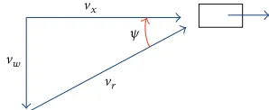
In the above equations,𝐴is the vehicle area,𝐿is the vehicle length,𝐿 = 𝑙_𝑓 + 𝑙_𝑟,𝜌is the density of air,V_𝑟 is the relative wind speed, and 𝐶_𝐹 and 𝐶_𝑀 are the force and moment nondimensional coefficients, respectively. The wind speed or crosswind is represented byV_𝑤 as shown in Figure 3. In

w

r

x

𝜓

Figure 3: Vehicle wind speed in crosswind situation.

general, crosswind can be at various angles, but, for simplicity, in this paper we will assume the crosswind to be at a 90-degree angle and will focus on the wind’s impact on the lateral forces and yaw torques [27].

The vehicle motion in ((1a), (1b), (1c), (1d), (1e))–(6) can be described by the following compact differential equation:

̇𝑥 = 𝐴𝑥 + 𝐵1𝑢 + 𝐵2𝑤 + 𝐵3𝑟,

𝑦 = 𝐶𝑥 + 𝐷𝑢 (7)

with𝑥 ∈ 𝑅𝑥,𝑢 ∈ 𝑅𝑢,𝑤 ∈ 𝑅𝑤,𝑟 ∈ 𝑅𝑟, and𝑦 ∈ 𝑅𝑦representing

the state vectors, control input vectors, crosswind effects as a disturbance vector, desired trajectory vectors, and measured output vectors, respectively. We define

𝑥 = [V_𝑦 𝑌 ̇𝜓 𝜓 ̇𝜙 𝜙 𝜔_𝑓 𝜔_𝑟]𝑇,

𝑢 = [𝛿𝑓 𝛿𝑟 𝑀𝑧]𝑇,

𝑤 = [𝐹𝑤 𝑀𝑤]𝑇,

𝑟 = [𝑌des 𝜓des]𝑇,

ℎ (𝜉) = [𝑌 𝜓]𝑇.

(8)

The state vectors represent the states for lateral velocity, lateral position, yaw rate, yaw angle, roll rate, roll angle, and front and rear wheels angular speed, respectively, and the output vectors represent lateral position and yaw angle.

3. Linear Model Predictive Control

(5)

Model predictive control

Linear tire model Reference

tracking

Dis

turba

n

ce Linear vehicle

model

x

Yref 𝛿f

𝛿r

Fx Fy

Y

Mz

𝜓_ref

𝜓

Figure 4: Predictive control structure.

faults can have substantial negative ramifications owing to the interconnected nature of processes [29].

In order to implement MPC with a receding horizon control strategy, the following strategy method is adopted:

(1) A dynamics process model is used to predict the behaviour of the plant and future plant outputs at each instant𝑘based on both previous and the latest observations of the system’s inputs and outputs. (2) The control signal inputs are calculated by

minimiz-ing the error of trackminimiz-ing between the predicted output and desired trajectory signal to keep the process as close as possible to following the trajectory, while considering the objective functions and constraints. (3) Only the first control signal is implemented on the

plant, whilst others are rejected in anticipation of the next sampling instant, where the future output will be known.

(4) Step (1) is repeated with updated values and all orders are updated.

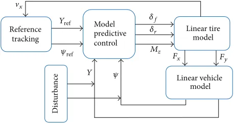
In this paper, we use the linear model of predictive control. The hierarchical control structure is adopted in MPC, as shown in Figure 4. Figure 4 illustrates the control structure for 2WS that uses front steering only,𝛿_𝑓, for 4WS that uses front and rear steering,𝛿_𝑓and 𝛿_𝑟, and for 2WS with DYC that produces external yaw moment (𝑀_𝑧) at both front and rear wheels as a control input to the system. These systems are used to control the vehicle in order to follow a given reference trajectory. They include the vehicle speed, desired reference trajectory, modelled predictive control, and linear vehicle model with linear tire model.

Using the equations from the vehicle and tire model, as explained and defined in (7), the basic equations of linear vehicle motion can be given as follows:

𝑚 ̇V𝑦= _𝐼 1

𝑥𝑥V𝑥[− (𝜇𝐶𝑟+ 𝐶𝑓) 𝐽𝑥𝑞V𝑦

+ (𝜇 (𝐶𝑟𝑙𝑟− 𝐶𝑓𝑙𝑓) 𝐽𝑥𝑞− 𝐼𝑥𝑥𝑚V2𝑥) ̇𝜓]

−_𝐼1

𝑥𝑥[(ℎ𝑏𝜙) ̇𝜙 − ℎ (𝑚𝑔ℎ − 𝑘𝜙) 𝜙 − 𝜇𝐶𝑓𝐽𝑥𝑞𝛿𝑓

+ 𝜇𝐶_𝑟𝐽_𝑥𝑞𝛿_𝑟]

(9a)

𝐼𝑧𝑧 ̈𝜓 = 1_V

𝑥[𝜇 (𝐶𝑟𝑙𝑟− 𝐶𝑓𝑙𝑓)V𝑦

− 𝜇 (𝐶𝑓𝑙𝑓2+ 𝐶𝑟𝑙𝑟2) ̇𝜓] + 𝜇𝐶𝑓𝑙𝑓𝛿𝑓− 𝜇𝐶𝑟𝑙𝑟𝛿𝑟

+ 𝑀𝑧

(9b)

𝐼_𝑥𝑥 ̈𝜙 = ℎ

V_𝑥[𝜇 (𝐶𝑟𝑙𝑟− 𝐶𝑓𝑙𝑓) ̇𝜓 − 𝜇 (𝐶𝑓+ 𝐶𝑟)V𝑦]

− 𝑏_𝜙 ̇𝜙 + (𝑚𝑔ℎ − 𝑘_𝜙) 𝜙 + 𝜇𝐶_𝑓ℎ𝛿_𝑓+ 𝜇𝐶_𝑟ℎ𝛿_𝑟,

(9c)

where𝐽_𝑥𝑞 = 𝐼_𝑥𝑥 + 𝑚ℎ2. A DYC that produces the reaction moment occurring at the front and rear wheels due to the steering angle effect (as an external yaw moments (𝑀_𝑧)) can be approximated with the following equations:

𝑀_𝑓≈ 2𝑙_𝑓𝐶_𝑓𝑀_𝑧,

𝑀_𝑟 ≈ 2𝑙_𝑟𝐶_𝑟𝑀_𝑧. (10)

We define front steering angle, rear steering angle, and direct yaw moment control as the inputs to the system. Thus, the vehicle motion can be represented in a given discrete state-space structure, as follows:

𝑥_𝑙(𝑘 + 1 | 𝑘) = 𝐴𝑙𝑥𝑙(𝑘 | 𝑘) + 𝐵𝑙𝑢𝑙(𝑘 | 𝑘)

+ 𝐵_𝑟𝑟_𝑙(𝑘 | 𝑘) ,

𝑦_𝑙(𝑘 | 𝑘) = 𝐶𝑙𝑥𝑙(𝑘 | 𝑘) + 𝐷𝑙𝑢𝑙(𝑘 | 𝑘) ,

(11)

where𝑥_𝑙(𝑘 | 𝑘)is the state vector at time step𝑘and 𝑥_𝑙(𝑘 +

1 | 𝑘)is the state vector at time step𝑘 + 1, with𝑥_𝑙(𝑘 | 𝑘) ∈

𝑅𝑥𝑙(𝑘|𝑘)_,𝑢

𝑅𝑦𝑙(𝑘|𝑘)_{representing the state vectors, control input vectors,}

reference vectors, and measured output vectors, respectively. We define

𝑥_𝑙(𝑘) = [V_𝑦 𝑌 ̇𝜓 𝜓 ̇𝜙 𝜙]𝑇,

𝑟_𝑙(𝑘) = [𝑌des 𝜓des]

𝑇_,

𝑦_𝑙(𝑘) = [𝑌 𝜓]𝑇.

(12)

For 2WS, 4WS, and 2WS with DYC, the control signal to the systems with the same tuning control parameters is given as follows:

𝑢_𝑙(𝑘) = [𝛿_𝑓] ,

𝑢_𝑙(𝑘) = [𝛿𝑓 𝛿𝑟]𝑇,

𝑢_𝑙(𝑘) = [𝛿𝑓 𝑀𝑧]𝑇.

(13)

We formulate the optimization of the predictive control system, which takes the constraints imposed on the input and input rate, respectively, as given in the following form:

−𝑢_𝑙≤ 𝑢_𝑙(𝑘) ≤ +𝑢𝑙,

−Δ𝑢_𝑙≤ Δ𝑢_𝑙(𝑘) ≤ +Δ𝑢𝑙.

(6)

One approach to maintain closed-loop stability would be to use all available control actuators (13) so that even if one of the control actuators fails, the rest can maintain closed-loop stability which the reliable control approaches. The use of redundant control actuators, however, incurs possibly pre-ventable operation and maintenance costs. These economic considerations dictate the use of only as many control loops as is required at a time. To achieve tolerance with respect to faults, control-loop reconfiguration can be carried out in the event of failure of the primary control configuration based on the assumption of a linear system.

Based on the linear vehicle model in (11) and by defining the outputs in (12), we consider the following cost functions to the system:

𝐽 (𝑥_𝑙(𝑘) , 𝑈_𝑙𝑘) =

𝐻𝑝 ∑

𝑖=1󵄩󵄩󵄩󵄩̃𝑦𝑙(𝑘 + 𝑖 | 𝑘) − 𝑟 (𝑘 + 𝑖 | 𝑘)󵄩󵄩󵄩󵄩

2 𝑄𝑖

+𝐻∑𝑐−1

𝑖=0 󵄩󵄩󵄩󵄩Δ̃𝑢𝑙(𝑘 + 𝑖 | 𝑘)󵄩󵄩󵄩󵄩

2 𝑅𝑖.

(15)

In (15), the first summation of the given cost function reflects the reduction of trajectory tracking errors among the predicted outputs̃𝑦_𝑙(𝑘 + 𝑖 | 𝑘)(𝑖 = 0, . . . , 𝐻_𝑝− 1) and the output reference signals𝑟(𝑘+𝑖 | 𝑘) (𝑖 = 0, . . . , 𝐻_𝑝−1), and the second summation reflects on the penalization of the control signal effortΔ̃𝑢_𝑙(𝑘 + 𝑖 | 𝑘)(𝑖 = 0, . . . , 𝐻_𝑐− 1) of the steering control manoeuvre. The aim of the predictive control system is to determine the optimal control input vectorΔ̃𝑢_𝑙(𝑘 + 𝑖 | 𝑘) so that the error function between the reference signal and the predicted output is reduced.

The difference in the steering angleΔ̃𝑢_𝑙(𝑘 + 𝑖 | 𝑘)is given in the case that the cost function is at a minimum value. The weight matrices𝑄(𝑖)and𝑅(𝑖)are semipositive definite and positive definite, respectively, and can be tuned for any desired closed-loop performance.𝑄(𝑖)is defined as the state tracking weight, since the error̃𝑦_𝑙(𝑘 + 𝑖 | 𝑘) − 𝑟(𝑘 + 𝑖 | 𝑘)can become as small as possible by increasing𝑄(𝑖). In a similar fashion, 𝑅(𝑖) represents the input tracking weight and the variation of the input is decreased to slow down the response of the system by increasing𝑅(𝑖). The predictive and control horizon are typically considered to be𝐻_𝑝 ≥ 𝐻_𝑐, while the control signal is considered constant for 𝐻_𝑐 ≤ 𝑖 ≤ 𝐻_𝑝. Matrices𝑄(𝑖)and𝑅(𝑖)represent the matrix weight of their appropriate dimensions for outputs and inputs, respectively, giving the state feedback control law as follows:

𝑢_𝑙(𝑘, 𝑦_𝑙(𝑘)) = 𝑢_𝑙(𝑘 − 1) + Δ𝑢_𝑙(𝑦_𝑙(𝑘)) . (16)

An optimal input was computed for the following time step rather than being calculated for the immediate time step by addressing convex optimization problems during each time step. After that, the first input is applied on the plant in (11), and the others are rejected, which yield the optimal control sequence as (16). The optimization problem in (15) is iterated with the new value at a time𝑘 + 1via new state𝑥(𝑘 + 1), and all orders are then updated.

The required direct yaw moment control𝑀_𝑧is obtained from the variation between the two sides of the vehicle torque,

as in (1e). In this research, the braking torque is only used based on the yaw rate; in other words, it is only activated in the case that the vehicle moves toward instability or in emergency manoeuvres, since it impacts the longitudinal motion, while the rear steering angle is assumed for the total manoeuvre to be in control or in standard driving manoeuvres. We take into account three control inputs, that is, front and rear steering angles, as well as differential braking at rear right and left tire, but only one control input is used at a time [30].

4. Simulation Results

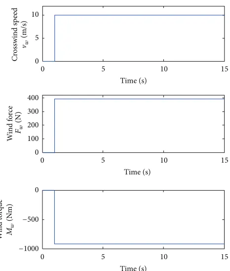
4.1. Scenario Description. The linear model predictive con-troller explained and presented was implemented for a vehicle path following a double-lane change scenario with a cross-wind effect present throughout the simulation. A double-lane change manoeuvre approximates as an emergency manoeu-vre case and generally demonstrates the agility and capabili-ties of the vehicle in lateral and roll dynamics. During such a manoeuvre, an understeering or oversteering, or even a roll-over situation, may occur. In this scenario, the vehicle is con-sidered travelling horizontally or straightforward, following the path with a constant velocity of 10 ms−1 and 30 ms−1 without braking or accelerating. The drag force and torque given by (6) in the initial driving conditions are assumed to act in the direction of the path at time𝑡 = 1sec with a wind velocity ofV_𝑤= 10ms−1. The forces and torques arising from this sidewise acting wind gust are assumed to be persistent and are applied as step functions throughout the simulation time, as shown in Figure 5. Table 1 shows the sport utility passenger car model parameters and their definitions used in this paper, based on Solmaz et al. [31].

For stability analysis, we simulated the system with only one input—in particular, the front steering angle𝛿_𝑓or 2WS. We set the vehicle velocity to be constant atV_𝑥 = 15ms−1; the road adhesion coefficient𝜇 = 1and wind velocityV_𝑤 =

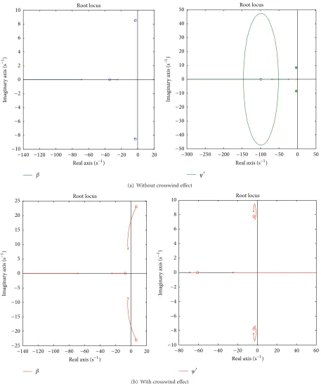
10ms−1. Figure 6(a) shows a stability analysis based on the root locus of the open-loop system in (7) showing matrix𝐴 without the crosswind effect (𝐵₂ = 0) and references signal (𝐵₃= 0). Those settings contribute to a stable region for both outputs (vehicle side slip and yaw rate responses). Matrix𝐴 is given in (8) with input signal being front steering angle (𝐵₁= 𝛿_𝑓). Since the root locus command in MATLAB is only working on the single-input single-output, therefore we eval-uate separately the output response with single input signal.

Figure 6(b) illustrates the effect of these factors: a cross-wind effect (𝐵₂ ̸= 0), references signal (𝐵₃ = 0), and con-trol signal (𝐵₁ = 0), with the same matrix𝐴as in (8) that yields unstable responses for both vehicle side slip and yaw rate. We can also notice that the poles are different for both cases due to 𝐵₂ matrices that are based on the crosswind effect. Furthermore, Figure 6(b) shows that within a wind velocity,V_𝑤= 10ms−1, the system is stable with the appropri-ate matrices of𝐴,𝐵₁, and𝐵₂. Figure 6(a) also illustrates that paired𝐴and𝐵₁are controllable, based on the model para-meters listed in Table 1.

(7)

0 5 10 15 0

5 10

Time (s)

Cr

osswind sp

eed

w

(m/s)

Time (s)

0 5 10 15

0 100 200 300 400

Wi

n

d

f

o

rc

e

Fw

(N)

Time (s)

0 5 10 15

0

−500

−1000

Wi

n

d

t

o

rq

u

e

Mw

(N

m)

Figure 5: Force and torque for crosswind speed of 10 ms−1.

Table 1: Car vehicle parameters.

Parameter Value

Car mass [kg] 1300

Inertia around the roll,𝑥-axis [kgm2] 370

Inertia around𝑧-axis [kgm2] 2167.56

Distance of front and rear wheels from centre of gravity (CoG) [m] 1.45, 1.07

Distance between the vehicle CoG and the assumed roll axis [m] 0.45

Equivalent suspension roll damping coefficient [Nms] 4200

Equivalent suspension roll stiffness coefficient [Nm] 40000

Linear approximation of tire stiffness for front and rear tire [N/rad] 133000, 121000

Gravitational constant [m/s2] 9.8

achieve the main aim, which is to follow the desired or refer-ence trajectory as close as possible. The controllers are com-pared against each other for 2DoF and 3DoF bicycle models, which excludes vehicle roll dynamics at various speeds, specifically low (10 ms−1) and high (30 ms−1), and also under wet concrete (𝜇 = 0.7) and icy (𝜇 = 0.1) road surfaces.

Since our study focused on an autonomous vehicle, it is reasonable to assume that the controllers will adapt to the road or environment, such as in the case of road adhesions, adverse weather, visual cues, traffic, and overall relevant driving conditions. Therefore, both controllers (2DoF and 3DoF) were designed and implemented with the parameters and conditions given in Tables 2, 3, and 4 for different vehicle forward speeds and road adhesion coefficients. The path-following tracking error is a measurement of how closely the output responses follow the reference trajectory, which is a measure of the deviation from the benchmark. In this

paper, we use the standard deviation of the root-mean square formula to calculate the tracking error, given by the following equation:

𝑒_𝑡= √Var(𝑦_𝑜− 𝑦_𝑟) = √ 1

(𝑛 − 1)∑ (𝑦𝑜− 𝑦𝑟)

2_, ₍₁₇₎

where 𝑒_𝑡 is the tracking error, 𝑛represents the number of time periods, and𝑦_𝑜and𝑦_𝑟express the measured output and reference.

(8)

0 50 0

10 20 30 40

50 Root locus

Im

agina

ry axis (s

−1 )

−10 −20 −30 −40 −50

−50 −100 −150 −200 −250 −300

Real axis (s−1)

𝜓󳰀

0 20

0 2 4 6 8

10 Root locus

Im

agina

ry axis (s

−1 )

−2 −4 −6 −8 −10

−20 −40 −60 −80 −100 −120 −140

Real axis (s−1)

𝛽

(a) Without crosswind effect

0 20 40 60

0 2 4 6 8

10 Root locus

Im

agina

ry axis (s

−1 )

Real axis (s−1)

−2 −4 −6 −8 −10

𝜓󳰀

−20 −40 −60 −80

0 20

0 5 10 15 20

25 Root locus

Im

agina

ry axis (s

−1)

−5 −10 −15 −20 −25

Real axis (s−1)

𝛽

−20 −40 −60 −80 −100 −120 −140

(b) With crosswind effect

Figure 6: Open-loop system in (7).

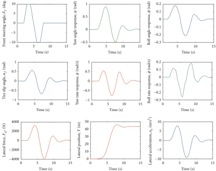
collision with other vehicles). We performed only the double-lane change and roll rate feedback fishhook test, for vehicle validation purposes in the open-loop simulation, as shown in Figures 7 and 8. The vehicle speed was set at 30 ms−1, which is suitable for both tests, with a road surface coefficient of 0.1. As illustrated in Figures 7 and 8, the vehicle response in terms

of yaw rate, roll rate, and lateral acceleration has been proven to be validated, thus being suitable for other simulations.

(9)

0 5 10 15 0

0.5 1

Time (s)

−0.5 −1

0 5 10 15

0 0.1 0.2

Time (s)

−0.1 −0.2 −0.3

0 5 10 15

0 0.5 1

Time (s)

−1 −0.5

Ti

re

s

lip

a

n

gl

e,

𝛼f

(rad)

0 5 10 15

0 0.5 1

Time (s)

−0.5

Y

aw a

n

gle r

esp

o

n

se

,

𝜓

(rad)

0 5 10 15

0 5 10

Time (s)

−5 −10

Front

s

te

er

in

g a

n

gl

e,

𝛿f

(deg.)

5 10 15

0 0.1 0.2

Time (s)

−0.1 −0.2 −0.3

Ro

ll a

n

gl

e r

esp

o

n

se

,

𝜙

(rad)

Time (s)

0 5 10 15

0 10 20 30 40 50

L

at

eral p

osi

tio

n

,

Y

(m)

0 5 10 15

0 2000 4000

Time (s)

−2000 −4000

L

at

eral f

o

rc

e,

Fyf

(N)

0 5 10 15

Time (s)

10 5 0 −5 −10

L

at

eral accelera

tio

n

,

ay

(m/s

2)

(rad/s)

Ro

ll ra

te

r

esp

o

n

se

,

̇_𝜙

(rad/s)

Y

aw ra

te

r

esp

o

n

se

,

̇_𝜓

Figure 7: Vehicle manoeuvre test of single-lane change at 30 ms−1with𝜇 = 0.1.

Table 2: Model predictive control parameters.

Parameter Value

Predictive horizon 20

Control horizon 9

Sampling time [s] 0.05

Constraints on max and min steering angles [deg.] ±20

Constraints on max and min changes in steering angles [deg./s] ±10

Constraints on max and min changes in moment torque [Nm/rad] ±2000

Constraints on max and min moment torque [Nm/rad/s] ±1500

Simulation time [s] 15

for controllers input and output were selected using trial-and-error method, where selection criteria were based on the best response output for both input and output for weighting gains.

The first simulation revolves around various road surface friction coefficients, from wet concrete (𝜇 = 0.7) to icy sur-face condition (𝜇 = 0.1), with a constant forward speed of 10 ms−1. The MPC weighting tuning parameters are listed in Table 3. We evaluated the controller’s robustness for the output responses by comparing the performance of 2WS, 4WS, and 2WS with DYC manoeuvres at a forward speed of

(10)

0 5 10 15 0

50 100

Time (s)

−50 −100

L

at

eral accelera

tio

n

,

ay

(m/s

2 )

Time (s)

0 5 10 15

0 1000 2000 3000

−1000

L

at

eral p

o

si

tio

n

,

Y

(m)

0 5 10 15

0 2 4

Time (s)

−2 −4

×104

L

at

eral f

o

rc

e,

Fyf

(N)

0 5 10 15

0 200 400

Time (s)

−200 −400

Front

s

te

er

in

g a

n

gl

e,

𝛿f

(deg.)

0 5 10 15

0 50 100 150 200

Time (s)

−50

Y

aw a

n

gle r

esp

o

n

se

,

𝜓

(rad)

5 10 15

0 1 2 3

Time (s)

−1 −2

Ro

ll a

n

gl

e r

esp

o

n

se

,

𝜙

(rad)

0 5 10 15

0 1 2

Time (s)

−1 −2

V

ehic

le sli

p

a

n

gl

e,

𝛽

(rad)

0 5 10 15

0 20 40 60

Time (s)

−20

0 5 10 15

0 5 10

Time (s)

−5

(rad/s)

Ro

ll ra

te

r

esp

o

n

se

,

̇_𝜙

(rad/s)

Y

aw ra

te

r

esp

o

n

se

,

̇_𝜓

Figure 8: Vehicle manoeuvre test of roll rate feedback at 30 ms−1with𝜇 = 0.1.

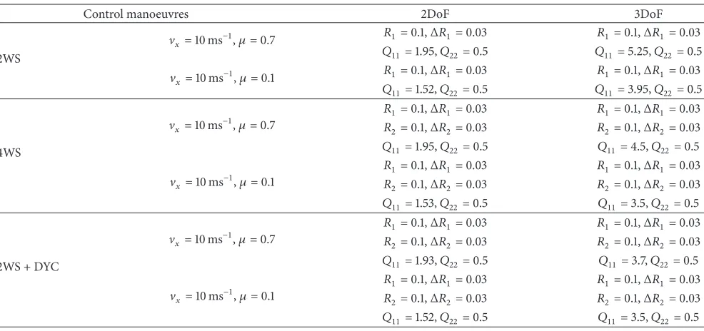
Table 3: Model predictive control weighting matrices parameters forV_𝑥 = 10 ms−1.

Control manoeuvres 2DoF 3DoF

2WS

V_𝑥= 10 ms−1,𝜇= 0.7 𝑅1= 0.1,Δ𝑅1 = 0.03 𝑅1= 0.1,Δ𝑅1 = 0.03

𝑄₁₁= 1.95,𝑄₂₂= 0.5 𝑄₁₁= 5.25,𝑄₂₂= 0.5

V_𝑥= 10 ms−1,𝜇= 0.1 𝑅1= 0.1,Δ𝑅1 = 0.03 𝑅1= 0.1,Δ𝑅1 = 0.03

𝑄11= 1.52,𝑄22= 0.5 𝑄11= 3.95,𝑄22= 0.5

4WS

V𝑥= 10 ms−1,𝜇= 0.7

𝑅₁= 0.1,Δ𝑅₁ = 0.03 𝑅₁= 0.1,Δ𝑅₁ = 0.03

𝑅₂= 0.1,Δ𝑅₂ = 0.03 𝑅₂= 0.1,Δ𝑅₂ = 0.03

𝑄₁₁= 1.95,𝑄₂₂= 0.5 𝑄₁₁= 4.5,𝑄₂₂= 0.5

V𝑥= 10 ms−1,𝜇= 0.1

𝑅₁= 0.1,Δ𝑅₁ = 0.03 𝑅₁= 0.1,Δ𝑅₁ = 0.03

𝑅2= 0.1,Δ𝑅2 = 0.03 𝑅2= 0.1,Δ𝑅2 = 0.03 𝑄11= 1.53,𝑄22= 0.5 𝑄11= 3.5,𝑄22= 0.5

2WS + DYC

V𝑥= 10 ms−1,𝜇= 0.7

𝑅₁= 0.1,Δ𝑅₁ = 0.03 𝑅₁= 0.1,Δ𝑅₁ = 0.03

𝑅₂= 0.1,Δ𝑅₂ = 0.03 𝑅₂= 0.1,Δ𝑅₂ = 0.03

𝑄₁₁= 1.93,𝑄₂₂= 0.5 𝑄₁₁= 3.7,𝑄₂₂= 0.5

V𝑥= 10 ms−1,𝜇= 0.1

(11)

Time (s)

0 5 10 15

0 0.5 1

4WS

−0.5 −1 −1.5 ×10−5

R

ear

ste

er

ing

ang

le,

𝛿r

(rad)

0 5 10 15

0 0.05 0.1

Time (s)

2WS 4WS 2WS + DYC

−0.05

−0.1

Front

s

te

er

in

g a

n

gl

e,

𝛿f

(rad)

0 5 10 15

0 1 2 3

Time (s)

2WS + DYC

−1 −2 −3 ×10−3

Dir

ec

t ya

w mo

men

t,

Mz

(N

m)

0 5 10 15

0 0.2

0 5 10 15

0 0.2 0.4

Time (s) Time (s)

Ref 2WS

4WS 2WS + DYC

Ref 2WS

4WS 2WS + DYC

−0.2

−0.4

−0.2

−0.4

Time (s)

0 5 10 15

0 2 4

Ref 2WS

4WS 2WS + DYC

−2

L

at

eral p

osi

tio

n

,

Y

(m)

Ya

w

a

n

gl

e,

𝜓

(rad)

Y

aw ra

te

,

𝜓

󳰀 (rad s −1 )

Figure 9: 2DoF controller at 10 ms−1and𝜇 = 0.7by 2WS, 4WS, and 2WS + DYC.

may be partly due to the fact that the rear steering and DYC were not used in lower speed manoeuvres.

Moreover, when the road surface friction was set to icy, the output responses from both controllers and all control manoeuvre techniques did not perfectly follow the desired trajectory as shown in Figures 10 and 11. 2WS with DYC yielded the best performance output compared to the others, especially in yaw rate response. 4WS was the next best, follow-ing 2WS, where the lateral position and yaw angle look almost identical. It seems that the rear steering and direct yaw moment controls were used in conjunction with front steer-ing for vehicle stabilization along the trajectory. However, from Table 5, the controller with 3DoF gives slightly better tracking error performance manoeuvres compared to con-troller 2DoF due to the fact that roll dynamics will not have much influence during low speed manoeuvres. Another fact is that, at low vehicle speed, all control inputs (front steering angle, rear steering angle, and direct yaw moment control) are under constraints.

Next, we tested the vehicle at various road friction coef-ficients again; however this time the vehicle was tested under a high forward speed of 30 ms−1. The same MPC design was used, of which the parameter controls are listed in Table 4. We compared the simulation results for 2WS, 4WS, and 2WS with DYC control manoeuvres for both controllers and present the comparison in Figures 12–15. The simulation results show

that, for 2DoF controller at 30 ms−1 and on wet concrete

(𝜇 = 0.7), all control manoeuvres give slightly similar

out-puts performances. Better responses were achieved in lateral positioning, and although the tracking performance of yaw angle and yaw rate deteriorated, the system still allowed the vehicle to track and follow the trajectory, successfully rejecting the effects of wind gust that impact the vehicle.

As tabulated in Table 6, 4WS and 2WS with DYC show slightly better tracking performance compared to 2WS only. However, in the case of the 3DoF controller, it can be clearly seen that 2WS with DYC and 4WS control manoeuvres offered a much higher performing response, especially in yaw angle and yaw rate response, than 2WS. This is shown in Figure 13. In this scenario, the rear steering and direct yaw moment control was fully utilized to control and enhance vehicle stability. It is therefore very important to consider roll dynamics in order to enhance vehicle stability and to follow the path trajectory. From Figures 12 and 13, there are some strong frequency oscillations in front of some responses; that is, front lateral force, vehicle side slip angle, and lateral acceleration trace, based on authors’ knowledge, come from the numerical calculation, or associated glitches, and initial condition of the system.

(12)

Time (s)

0 5 10 15

0 2 4

Ref 2WS

4WS 2WS + DYC

−2

L

at

eral p

o

si

tio

n

,

Y

(m)

0 5 10 15

0 0.2 0.4

Time (s)

Ref 2WS

4WS 2WS + DYC

−0.2

−0.4

Y

aw ra

te

,

𝜓

󳰀(rad s −1)

0 5 10 15

0 0.2

Time (s)

Ref 2WS

4WS 2WS + DYC

−0.2

−0.4

Ya

w

a

n

gl

e,

𝜓

(rad)

Time (s)

0 5 10 15

0 0.1

4WS

−0.1

−0.2

Rea

r s

teerin

g a

n

gle

,

𝛿r

(rad)

0 5 10 15

0 0.05 0.1

Time (s)

2WS 4WS 2WS + DYC

−0.05

−0.1

Front

s

te

er

in

g a

n

gl

e,

𝛿f

(rad)

0 5 10 15

0 0.1 0.2

Time (s)

2WS + DYC

−0.1

−0.2

Dir

ec

t ya

w mo

men

t,

Mz

(N

m)

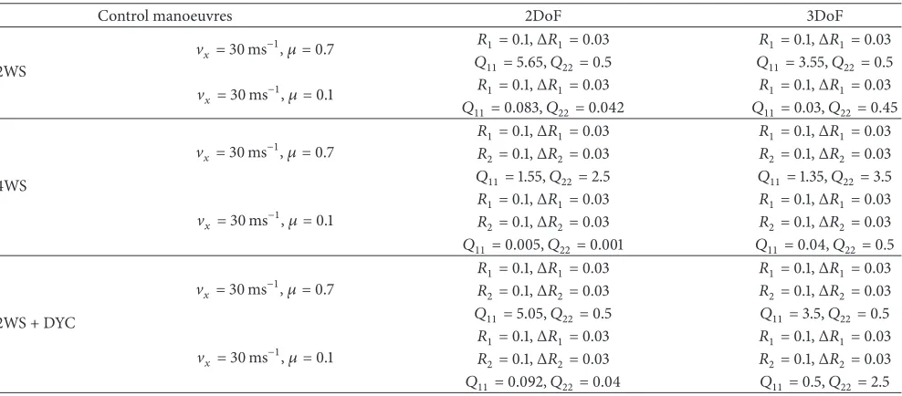
Table 4: Model predictive control weighting matrices parameters forV_𝑥= 30 ms−1.

Control manoeuvres 2DoF 3DoF

2WS

V𝑥 =30 ms−1,𝜇= 0.7 _𝑄𝑅1= 0.1,Δ𝑅1 = 0.03 𝑅1 = 0.1,Δ𝑅1 = 0.03 11= 5.65,𝑄22= 0.5 𝑄11= 3.55,𝑄22= 0.5 V_𝑥 =30 ms−1,𝜇= 0.1 𝑅1= 0.1,Δ𝑅1 = 0.03 𝑅1 = 0.1,Δ𝑅1 = 0.03

𝑄11= 0.083,𝑄22= 0.042 𝑄11= 0.03,𝑄22= 0.45

4WS

V_𝑥 =30 ms−1,𝜇= 0.7

𝑅1= 0.1,Δ𝑅1 = 0.03 𝑅1 = 0.1,Δ𝑅1 = 0.03 𝑅2= 0.1,Δ𝑅2 = 0.03 𝑅2 = 0.1,Δ𝑅2 = 0.03 𝑄₁₁= 1.55,𝑄₂₂= 2.5 𝑄₁₁= 1.35,𝑄₂₂= 3.5

V_𝑥 =30 ms−1,𝜇= 0.1

𝑅1= 0.1,Δ𝑅1 = 0.03 𝑅1 = 0.1,Δ𝑅1 = 0.03 𝑅2= 0.1,Δ𝑅2 = 0.03 𝑅2 = 0.1,Δ𝑅2 = 0.03 𝑄₁₁= 0.005,𝑄₂₂= 0.001 𝑄₁₁= 0.04,𝑄₂₂= 0.5

2WS + DYC

V_𝑥 =30 ms−1,𝜇= 0.7

𝑅1= 0.1,Δ𝑅1 = 0.03 𝑅1 = 0.1,Δ𝑅1 = 0.03 𝑅₂= 0.1,Δ𝑅₂ = 0.03 𝑅₂ = 0.1,Δ𝑅₂ = 0.03

𝑄11= 5.05,𝑄22= 0.5 𝑄11= 3.5,𝑄22= 0.5

V_𝑥 =30 ms−1,𝜇= 0.1

𝑅1= 0.1,Δ𝑅1 = 0.03 𝑅1 = 0.1,Δ𝑅1 = 0.03 𝑅₂= 0.1,Δ𝑅₂ = 0.03 𝑅₂ = 0.1,Δ𝑅₂ = 0.03

𝑄₁₁= 0.092,𝑄₂₂= 0.04 𝑄₁₁= 0.5,𝑄₂₂= 2.5

simulation; the tracking responses become unstable and impossible to control, especially under the crosswind effect as shown in Figure 14. The most probable cause is the roll dynamic motion neglect in the 2DoF controller design, when the vehicle itself was modelled by including roll dynamic factor. It can be said that the inclusion of roll dynamic factor

(13)

0 5 10 15 0

2 4

Time (s)

Ref 2WS

4WS 2WS + DYC

−2

L

at

eral p

o

si

tio

n

,

Y

(m)

0 5 10 15

0 0.2 0.4

Time (s)

Ref 2WS

4WS 2WS + DYC

−0.2 −0.4

Y

aw ra

te

,

𝜓

󳰀 (rad s −1 )

0 5 10 15

0 0.2

Time (s)

Ref 2WS

4WS 2WS + DYC

−0.2

−0.4

Ya

w

a

n

gl

e,

𝜓

(rad)

0 5 10 15

0 0.1

Time (s)

4WS

−0.1

−0.2

Rea

r s

teerin

g a

n

gle

,

𝛿r

(rad)

0 5 10 15

0 0.05 0.1

Time (s)

2WS 4WS 2WS + DYC

−0.05 −0.1

Front

s

te

er

in

g a

n

gl

e,

𝛿f

(rad)

0 5 10 15

0 0.02 0.04

Time (s)

2WS + DYC

−0.02 −0.04 −0.06

Dir

ec

t ya

w mo

men

t,

Mz

(N

m)

Table 5: Path following tracking errors with road friction surface𝜇= 0.7.

Vehicle speed Manoeuvre control Controller 2DoF Controller 3DoF

𝑌[m] Ψ[rad] 𝑌[m] Ψ[rad]

10

2WS 0.0637 0.0085 0.0623 0.0074

4WS 0.0548 0.0054 0.0526 0.0051

2WS + DYC 0.0542 0.0051 0.0527 0.0051

30

2WS 0.0639 0.5348 0.0616 0.5215

4WS 0.0558 0.5239 0.0528 0.0023

2WS + DYC 0.0549 0.5226 0.0524 0.0254

by the linear tire model. These results show that linear tire model is only suitable for analyzing a stable vehicle behaviour under the assumption of small steering and acceleration.

Next, for the 3DoF controller simulation, 2WS with DYC manoeuvres provides a much better tracking response in comparison to 4WS, particularly in the case of lateral output. On the contrary, 4WS manoeuvre demonstrates a much bet-ter tracking response in the yaw angle and yaw rate responses, as tabulated in Table 6. With appropriate weight tuning gain, the rear steering angle and direct yaw moment control are fully optimized in order to become stable along the given tra-jectory. However, for the 2WS manoeuvre, the vehicle responses become unstable, despite several instances where the weighting tuning gains are adjusted for output and input gains. With the inclusion of another input control to the con-troller design, we can enhance the vehicle responses for both

(14)

0 5 10 15 0

2 4

Time (s)

Ref 2WS

4WS 2WS + DYC

−2

L

at

eral p

osi

tio

n

,

Y

(m)

0 5 10 15

0 0.2

Time (s)

Ref 2WS

4WS 2WS + DYC

−0.2

−0.4

Ya

w

a

n

gl

e,

𝜓

(rad)

0 5 10 15

0 0.2 0.4

Time (s)

Ref 2WS

4WS 2WS + DYC

−0.2 −0.4

Y

aw ra

te

,

𝜓

󳰀 (rad s −1 )

0 5 10 15

0 1000 2000

Time (s)

2WS 4WS 2WS + DYC

−1000 −2000

F

ro

n

t la

teral f

o

rc

e,

Fyf

(N

m)

0 5 10 15

0 0.01 0.02

Time (s)

2WS 4WS 2WS + DYC

−0.01

V

ehic

le side sli

p

,

𝛽

(rad)

0 5 10 15

0 1 2

Time (s)

2WS 4WS 2WS + DYC

−1 −2

L

at

eral accelera

tio

n

,

ay

(m

s

−2)

0 5 10 15

0 0.01 0.02 0.03

Time (s)

2WS 4WS 2WS + DYC

−0.01 −0.02

Front

s

te

er

in

g a

n

gl

e,

𝛿f

(rad)

0 5 10 15

0 0.0005 0.001

4WS Time (s)

−0.0005 −0.001 −0.0015

Rea

r s

teerin

g a

n

gle

,

𝛿r

(rad)

0 5 10 15

0 0.01 0.02

Time (s)

2WS + DYC

−0.01 −0.02

Dir

ec

t ya

w mo

men

t,

Mz

(N

m)

for lateral response and neither 2WS nor 2WS with DYC control manoeuvres for yaw angle or yaw rate response performed well, causing an increase in vehicle instability, increased vibration, and tracking responses deterioration. We will next focus on how to enhance the controller in order to stabilize vehicle manoeuvrability and handling stability.

We can therefore conclude that, for 4WS, the rear wheels were helping the car to steer by improving the vehicle handling at high speed, while decreasing the turning radius at low speed, as shown by the control signal in Figures 12 and 13. Meanwhile, for 2WS with DYC, active front steering was used in low speed manoeuvres for lateral acceleration, while inclusion of DYC was adopted for high lateral acceleration when the tires were saturated and could not produce enough lateral force for vehicle control and stability as intended. In 2WS vehicles, the rear set of wheels do not play an

(15)

0 5 10 15 0

2 4

Ref 2WS

4WS 2WS + DYC Time (s)

−2

L

at

eral p

osi

tio

n

,

Y

(m)

0 5 10 15

0 0.2

Ref 2WS

−0.2

−0.4

Ya

w

a

n

gl

e,

𝜓

(rad)

0 5 10 15

0 0.2 0.4

Ref 2WS

−0.2 −0.4

Y

aw ra

te

,

𝜓

󳰀(rad s −1)

0 5 10 15

0 1000 2000

2WS 4WS 2WS + DYC

Time (s)

−1000

−2000

F

ro

n

t la

teral f

o

rc

e,

Fyf

(N

m)

0 5 10 15

0 0.1 0.2 0.3

2WS 4WS 2WS + DYC

Time (s)

−0.1 −0.2

V

ehic

le side sli

p

,

𝛽

(rad)

0 5 10 15

0 5 10

2WS 4WS 2WS + DYC

Time (s)

−5

−10

L

at

eral accelera

tio

n

,

ay

(m

s

−2)

0 5 10 15

0 0.1 0.2 0.3

2WS 4WS 2WS + DYC

Time (s)

−0.1 −0.2

Front

s

te

er

in

g a

n

gl

e,

𝛿f

(rad)

0 5 10 15

0 0.1 0.2 0.3

4WS Time (s)

−0.1 −0.2

Rea

r s

teerin

g a

n

gle

,

𝛿r

(rad)

0 5 10 15

0 0.05 0.1

2WS + DYC Time (s)

−0.05 −0.1

Dir

ec

t ya

w mo

men

t,

Mz

(N

m)

Table 6: Path following tracking errors with road friction surface𝜇= 0.1.

Vehicle speed Manoeuvre control Controller 2DoF Controller 3DoF

𝑌[m] Ψ[rad] 𝑌[m] Ψ[rad]

10

2WS 0.0874 0.0115 0.0841 0.0104

4WS 0.0838 0.0109 0.0832 0.0094

2WS + DYC 0.0838 0.0110 0.0835 0.0083

30

2WS Uncontrolled Uncontrolled 2.1352 0.5264

4WS Uncontrolled Uncontrolled 0.8824 0.2982

(16)

0 10 20 30 0 2 4 6 8 10 Time (s) Ref 2WS 4WS 2WS + DYC

−2 −4 L at eral p osi tio n , Y (m)

0 10 20 30

0 0.2 0.4 Time (s) Ref 2WS 4WS 2WS + DYC

−0.2 −0.4 Ya w a n gl e, 𝜓 (rad)

0 10 20 30

0 0.2 0.4 0.6 Time (s) Ref 2WS 4WS 2WS + DYC

−0.2 −0.4 −0.6 Y aw ra te , 𝜓

󳰀 (rad s −1 )

0 10 20 30

0 0.5 1 1.5 Time (s) 2WS 4WS 2WS + DYC

−0.5 −1 −1.5

V

ehic

le side sli

p

,

𝛽

(rad)

0 10 20 30

0 2 4 Time (s) 2WS 4WS 2WS + DYC

−2 −4 L at eral accelera tio n , ay (m s −2)

0 10 20 30

0 0.2 0.4 0.6 Time (s) 2WS 4WS 2WS + DYC

−0.2 −0.4 Front s te er in g a n gl e, 𝛿f (rad)

0 10 20 30

0 0.2 0.4 0.6 Time (s) 4WS −0.2 Rea r s teerin g a n gle , 𝛿r (rad)

0 10 20 30

0 0.05 0.1

Time (s)

2WS + DYC

−0.05 Dir ec t ya w mo men t, Mz (N m)

0 10 20 30

0 0.5 1 1.5 Time (s) 2WS 4WS 2WS + DYC

−0.5 −1 −1.5 F ro n t la teral f o rc e, Fyf (N m) ×104

5. Conclusion

This paper presents the robustness of model predictive con-trol for an autonomous ground vehicle on a path-following control, with consideration of wind gust effects subjected to the variation of forward speeds and road surfaces condi-tion, in a double-lane change scenario. The predictive con-trollers were designed based on two- (lateral-yaw model) and three- (lateral-roll model) degree-of-freedom vehicle models. The only difference between the models is the roll dynamics factor, which is taken into consideration, and both controllers were implemented into a six-degree-of-free-dom vehicle model. Based on linear vehicle and tire model approximations of a known trajectory, we evaluated the effect and impact of roll dynamics at low and high forward vehicle

speeds and at various road frictions (wet concrete to icy roads) in order to follow a desired trajectory as close as pos-sible while rejecting the crosswind effects and maintaining vehicle stability. We also evaluated and compared the effi-ciency of the different manoeuvres via two-wheel steering, four-wheel steering, and two-wheel steering with direct yaw moment control.

(17)

0 10 20 30 0

5

Time (s)

Ref 2WS

4WS 2WS + DYC

−10 −5

−15

L

at

eral p

osi

tio

n

,

Y

(m)

0 10 20 30

0 0.2

Time (s)

Ref 2WS

4WS 2WS + DYC

−0.2

−0.4

Ya

w

a

n

gl

e,

𝜓

(rad)

0 10 20 30

0 0.25 0.5

Time (s)

Ref 2WS

4WS 2WS + DYC

−0.25 −0.5

Y

aw ra

te

,

𝜓

󳰀(rad s −1)

0 10 20 30

0 500 1000

Time (s)

2WS 4WS 2WS + DYC

−500 −1000 −1500

F

ro

n

t la

teral f

o

rc

e,

Fyf

(N

m)

0 10 20 30

0 0.1 0.2 0.3 0.4

Time (s)

2WS 4WS 2WS + DYC

−0.1 −0.2

V

ehic

le side sli

p

,

𝛽

(rad)

0 10 20 30

0 2 4

Time (s)

2WS 4WS 2WS + DYC

−2 −4

L

at

eral accelera

tio

n

,

ay

(m

s

−2)

0 10 20 30

0 0.1 0.2 0.3 0.4

Time (s)

2WS 4WS 2WS + DYC

−0.1 −0.2

Front

s

te

er

in

g a

n

gl

e,

𝛿f

(rad)

0 10 20 30

0 0.1 0.2 0.3

Time (s)

4WS

−0.1 −0.2

Rea

r s

teerin

g a

n

gle

,

𝛿r

(rad)

0 10 20 30

0 2 4

Time (s)

2WS + DYC

−2 −4 ×10−4

Dir

ec

t ya

w mo

men

t,

Mz

(N

m)

the car by improving the vehicle handling at high speed, decreasing the turning radius at low speeds, and reducing the tracking error for lateral position and yaw angle response.

The simulation also demonstrated that model predictive control has an ability to reject the side wind effect as a disturbance to the system, which is particularly effective at 10 ms−1 for all cases, except for the 2DoF controller during simulation of higher speeds on lower road surface adhesion. However, both controllers were not able to provide a better response when the vehicle performed at a high forward speed with a low road adhesion coefficient; particularly, when 2DoF controller was simulated, all results showed unstable vehicle response. Thus, for this scenario, we are currently investigating new approaches with a real-time implementable

control scheme. Further improvement for future works on control methodology will also be considered to minimize tracking error and to enhance vehicle stability.

Competing Interests

The authors declare that they have no competing interests.

Acknowledgments

(18)

References

[1] E. F. Camacho and C. Bordons, Model Predictive Control, Springer, London, UK, 2nd edition, 2007.

[2] C. E. Garc´ıa, D. M. Prett, and M. Morari, “Model predictive con-trol: theory and practice—a survey,”Automatica, vol. 25, no. 3, pp. 335–348, 1989.

[3] P. Mhaskar, “Robust model predictive control design for fault-tolerant control of process systems,”Industrial & Engineering Chemistry Research, vol. 45, no. 25, pp. 8565–8574, 2006. [4] V. Vesely and D. Rosinova, “Robust model predictive control

design,” inModel Predictive Control, T. Zheng, Ed., pp. 1–24, InTech, Rijeka, Croatia, 2010.

[5] M. Nagai, M. Shino, and F. Gao, “Study on integrated control of active front steer angle and direct yaw moment,”JSAE Review, vol. 23, no. 3, pp. 309–315, 2002.

[6] F. Yakub and Y. Mori, “Comparative study of autonomous path-following vehicle control via model predictive control and linear quadratic control,”Proceedings of the Institution of Mechanical Engineers, Part D, vol. 229, no. 12, pp. 1695–1714, 2015. [7] C. March and T. Shim, “Integrated control of suspension and

front steering to enhance vehicle handling,”Proceedings of the Institution of Mechanical Engineers, Part D: Journal of Auto-mobile Engineering, vol. 221, no. 4, pp. 377–391, 2007.

[8] J. Wang, D. A. Wilson, W. Xu, and D. A. Crolla, “Integrated vehicle ride and steady-state handling control via active suspen-sions,”International Journal of Vehicle Design, vol. 42, no. 3-4, pp. 306–327, 2006.

[9] M. J. L. Boada, B. L. Boada, A. Mu˜noz, and V. D´ıaz, “Integrated control of front-wheel steering and front braking forces on the basis of fuzzy logic,”Proceedings of the Institution of Mechanical Engineers, Part D: Journal of Automobile Engineering, vol. 220, no. 3, pp. 253–267, 2006.

[10] A. Balluchi, A. Bicchi, and P. Sou`eres, “Path-following with a bounded-curvature vehicle: a hybrid control approach,” Inter-national Journal of Control, vol. 78, no. 15, pp. 1228–1247, 2005. [11] K. Moriwaki, “Autonomous steering control for electric vehicles

using nonlinear state feedback𝐻_∞control,”Nonlinear Analysis, Theory, Methods and Applications, vol. 63, no. 5–7, pp. e2257– e2268, 2005.

[12] B. Mashadi, P. Ahmadizadeh, and M. Majidi, “Integrated con-troller design for path following in autonomous vehicles,” SAE Technical Paper 2011-01-1032, SAE International, 2011. [13] J.-M. Park, D.-W. Kim, Y.-S. Yoon, H. J. Kim, and K.-S. Yi,

“Obstacle avoidance of autonomous vehicles based on model predictive control,”Proceedings of the Institution of Mechanical Engineers, Part D: Journal of Automobile Engineering, vol. 223, no. 12, pp. 1499–1516, 2009.

[14] Y. Yoon, J. Shin, H. J. Kim, Y. Park, and S. Sastry, “Model-pre-dictive active steering and obstacle avoidance for autonomous ground vehicles,”Control Engineering Practice, vol. 17, no. 7, pp. 741–750, 2009.

[15] P. Falcone, F. Borrelli, J. Asgari, H. E. Tseng, and D. Hrovat, “Pre-dictive active steering control for autonomous vehicle systems,” IEEE Transactions on Control Systems Technology, vol. 15, no. 3, pp. 566–580, 2007.

[16] T. Keviczky, P. Falcone, F. Borrelli, J. Asgari, and D. Hrovat, “Predictive control approach to autonomous vehicle steering,” inProceedings of the American Control Conference, pp. 4670– 4675, IEEE, Minneapolis, Minn, USA, June 2006.

[17] F. Borrelli, P. Falcone, T. Keviczky, J. Asgari, and D. Hrovat, “MPC-based approach to active steering for autonomous

vehicle systems,”International Journal of Vehicle Autonomous Systems, vol. 3, no. 2–4, pp. 265–291, 2005.

[18] K. Nam, S. Oh, H. Fujimoto, and Y. Hori, “Robust yaw stability control for electric vehicles based on active front steering con-trol through a steer-by-wire system,”International Journal of Automotive Technology, vol. 13, no. 7, pp. 1169–1176, 2012. [19] H. Yoshida, S. Shinohara, and M. Nagai, “Lane change steering

manoeuvre using model predictive control theory,” Vehicle System Dynamics, vol. 46, no. 1, pp. 669–681, 2008.

[20] P. Falcone, H. Eric Tseng, F. Borrelli, J. Asgari, and D. Hrovat, “MPC-based yaw and lateral stabilisation via active front steering and braking,”Vehicle System Dynamics, vol. 46, no. 1, pp. 611–628, 2008.

[21] W. Kim, D. Kim, K. Yi, and H. J. Kim, “Development of a path-tracking control system based on model predictive control using infrastructure sensors,”Vehicle System Dynamics, vol. 50, no. 6, pp. 1001–1023, 2012.

[22] B.-C. Chen and H. Peng, “Differential-braking-based rollover prevention for sport utility vehicles with human-in-the-loop evaluations,”Vehicle System Dynamics, vol. 36, no. 4-5, pp. 359– 389, 2001.

[23] G. Palmieri, P. Falcone, H. E. Tseng, and L. Glielmo, “A prelim-inary study on the effects of roll dynamics in predictive vehicle stability control,” inProceedings of the 47th IEEE Conference on Decision and Control (CDC ’08), pp. 5354–5359, IEEE, Cancun, Mexico, December 2008.

[24] H. Pacejka,Tire and Vehicle Dynamics, Elsevier, Oxford, UK, 3rd edition, 2012.

[25] R. N. Jazar,Vehicle Dynamics Theory and Application, Springer, New York, NY, USA, 3rd edition, 2009.

[26] C. R. Carlson and J. C. Gerdes, “Optimal rollover prevention with steer by wire and differential braking,” inProceedings of the ASME International Mechanical Engineering Congress, vol. 1, no. 1, pp. 345–354, Washington, Wash, USA, November 2003. [27] C. J. Baker, “Measures to control vehicle movement at exposed

sites during windy periods,”Journal of Wind Engineering and Industrial Aerodynamics, vol. 25, no. 2, pp. 151–161, 1987. [28] M. Mahmood and P. Mhaskar, “On constructing constrained

control Lyapunov functions for linear systems,”IEEE Transac-tions on Automatic Control, vol. 56, no. 5, pp. 1136–1140, 2011. [29] M. Mahmood and P. Mhaskar, “Enhanced stability regions for

model predictive control of nonlinear process systems,”AIChE Journal, vol. 54, no. 6, pp. 1487–1498, 2008.

[30] F. Yakub and Y. Mori, “Heavy vehicle stability and rollover pre-vention via switching model predictive control,”International Journal of Innovative Computing, Information and Control, vol. 11, no. 5, pp. 1751–1764, 2015.

[31] S. Solmaz, M. Corless, and R. Shorten, “A methodology for the design of robust rollover prevention controllers for automotive vehicles with active steering,”International Journal of Control, vol. 80, no. 11, pp. 1763–1779, 2007.

(19)

International Journal of