PARAMETER ESTIMATION OF TAPIOCA STARCH
HYDROLYSIS PROCESS: APPLICATION OF LEAST SQUARES
AND GENETIC ALGORITHM
Roslina Rashid1, Hishamuddin Jamaluddin2and Nor Aishah Saidina Amin1 1Faculty of Chemical and Natural Resources Engineering,
2Faculty of Mechanical Engineering, Universiti Teknologi Malaysia, 81310 UTM, Skudai, Johor.
ABSTRACT
The performance of genetic algorithm (GA) in nonlinear kinetic parameter estimation of tapioca starch hydrolysis was studied and compared with the Gauss-Newton method. Both methods were employed for determining the model parameters of the modified version of Gonzalez-Tello model. To estimate and validate the model parameters, experimental works involving hydrolysing tapioca starch were conducted. The model was then used to predict glucose concentration profile for a given initial condition of the tapioca hydrolysis process. In terms of error index values, both methods produced good results. This study showed that the impact of user defined parameters of the GA was insignificant as compared with the influence of initial parameters of the Gauss-Newton method on the predictive performance. Furthermore, the GA approach requires no guessing of the initial values and is able to produce reasonable solutions for the estimated parameters.
Keywords : Gauss-Newton Method, Genetic Algorithm, Mathematical Model, Parameter Estimation, Starch Hydrolysis
1.0 INTRODUCTION
Starch hydrolysis process is known as a process that can produce a wide range of products such as maltodextrin, mixed syrups, high maltose syrups and glucose syrups. Those products are different in their glucose content. The whole purpose of modeling this process is to predict the future glucose concentration for a given initial condition of the process. In order to solve the mathematical model, attention is drawn to determine (or estimate) and validate the model parameters of the tapioca starch hydrolysis process.
Many studies on the modeling of akin process have been reported [1-3]. From previous findings, the mathematical modeling of the hydrolysis process leads to a nonlinear parameter estimation problem and the model parameters of the process have been determined either using conventional graphical-based technique [4] or nonlinear regression method [5]. However, the usual approach to estimate model parameters of a biological process is by using nonlinear techniques since the graphical methods have shown inferior parameter estimates compared to those generated using nonlinear techniques [6]. On the other hand, the nonlinear techniques also have their drawbacks. This scheme often fails in the search for global optimum if the search space is non linear in parameters [7]. For a large value of least squares sum, a slow convergence often appears [8]. A common practice to deal with the local convergence problem is to test different initial guess parameters. However, the probability of finding an initial condition suitable for all parameters decreases as the number of involved parameter, increases [9]. Because of the limitations imposed by those methods, an attempt was made to estimate the model parameters of the tapioca starch hydrolysis using genetic algorithm.
Marteijn et al. [10] utilised GA to optimise the feed medium composition for fed-batch culture of insect cells. Na et al. [11] used GA to determine the feed rate profile for production of salmon calcitonin (intracellular protein) and Park
et al. [12] utilised GA to estimate the kinetic parameters of Catharanthus roseus and Nicotiana tabacum fermentation. Although many studies [11-13] have been done by using GA for parameter estimation in bioprocesses, application of GA for determining the kinetics parameters of the starch empirical model has not been explored. This study attempts to estimate the parameters using GA and to compare the results with those calculated using the Gauss-Newton method. The contribution of this paper is to present the application of GA method for determination of the coefficients of the empirical model in an objective manner, and to compare the results obtained by GA with the results obtained by the Gauss-Newton method.
The organisation of this paper is as follows. The experimental work carried out on the process is described in experimental works section, while the kinetic model of the hydrolysis process was explained in the kinetic model section. Then the parameter estimation problem section describes the Gauss-Newton and Genetic algorithm procedures followed by a section presenting results and discussions for both methods (GA and Gauss Newton). The last section gives the conclusions drawn from this study.
2.0 EXPERIMENTAL WORK
Experiments were performed to obtain data (reaction profiles) for estimating and validating the model parameters. In the present study, tapioca starch was hydrolysed in two separate steps: liquefaction and saccharification. Initial dry solid and enzyme dosage were chosen as the initial conditions for the experimental design because they strongly influence the production of glucose. The methodology of liquefaction and saccharification were followed as reported previously [1,14].
2.1 LIQUEFACTION
commercial enzyme Termamyl 120L Type S produced by submerged fermentation of a genetically modified Bacillus licheniformis micro-organism manufactured by Novo Company in the United States. 1L starch slurry (10 - 40% ds,w/v) with distilled water was prepared in 2L Schott Bottle. Calcium chloride dehydrate (40 ppm) and 0.055% alpha-amylase (w/w based on dry solid) were added to the slurry. The slurry pH was adjusted to 6.2 (pH range from 6.0 - 6.5) with 2M NaOH. The mixture was heated to 80˚C for 5 minutes to fully gelatinise the starch. The mixture was then transferred to a 2L reactor for dextrination process. This process was maintained at 95˚C for 2 hours and the mixing speed was at 200 rpm. During this stage, alpha-amylase reacts with the starch to produce dextrin. After 2 hours of liquefaction, the pH of the mixture was adjusted to 3 with 2M HCl at 95˚C for 10 minutes. This step is to ensure inactivation of the residual alpha-amylase after liquefaction.
2.2 SACCHARIFICATION
The saccharification process was carried out soon after liquefaction and cooled rapidly to the saccharification temperature to avoid retrogradation. In the saccharification step, pH was adjusted to 4.3 (pH was not allowed to drop below 3.5) at 60ºC. The commercial enzyme, AMG E was used. AMG E (EC 3.2.13) is an amyloglucosidase produced by a genetically modified strain of an Aspergillus Niger microorganism. The amount of the enzyme was varied from 0.7 to 1.2 L/ton starch. During the course of the hydrolysis, 1 ml sample was drawn from the reactor every 10 minutes for 10 hours followed by sampling after 23 and 24 hours. The sample was then heated to 80˚C for approximately 20 minutes to cease any remaining amyglucosidase activity.
2.3 ANALYSIS METHOD
The amount of reducing sugar was determined by the dinitrosalicylic acid (DNS) method [15]. 2 ml distilled water and 1 ml DNS reagent were added to the 1 ml sample and placed in a water bath at 80˚C for about 5 minutes to allow reaction to occur between DNS and glucose. Each volume was adjusted to 10 ml accurately with distilled water and mixed well. The samples were analysed at 540 nm using 2 spectrophotometer.
3.0 KINETIC MODEL
In this study, the rate of glucose production is described using a modified version of an empirical model developed earlier [5]. The empirical model is considered because it has been proven suitable for similar processes. The study showed that the overall rate of enzyme hydrolysis could be successfully represented by
(1)
where a and b are kinetic parameters of the process, x is a dimensionless conversion and c is a constant. Based on the experimental data, a, band cfor tapioca starch hydrolysis were estimated. Earlier investigations [5] showed that a is a function of enzyme dosage and temperature and bis equal to 8.75. The product concentrations G, is related to the dimensionless
conversion xby
(2)
where G (mg/L) represents the glucose concentration and S0
(mg/L) is the initial dry solid. By integrating equation (1) between an initial value (t0, x0) and at any given instant (t, x),
the following equation is obtained:
(3)
The term exp(bx) of Equation 3 is expanded using Taylor series expansion and evaluated at xo. Then, each term of the
expansion is divided by (c+x) before integrating each of the expression. Thus, the integral expression in Equation 3 can be approximated by the series expansion evaluated about x0
given by
(4)
Finally, Equations 4 is substituted into equation (3) and the following equation is obtained:
(5)
Only three terms in the left hand side of eequation 5 were considered since the truncation errors due to other terms are insignificant. The Gauss-Newton method was then utilised to estimate the parameters a, band cin equation (5) from the measured values x. The estimated parameters were then substituted into Equation 1 and the equation was solved numerically using Runge-Kutta method to obtain the conversion profile and compared with the experimental data.
4.0 PARAMETER ESTIMATION PROBLEM
(6)
where e is the residual between the estimated and observed value of glucose concentration and yis the observed value of glucose concentration.
4.1 GAUSS-NEWTON METHOD
In the present work, the Gauss-Newton algorithm of non-linear least squares problem was utilised to estimate the parameters a, b and c of Equation 5. MATLAB statistical toolbox (version 5.3) was utilised to implement the parameter estimation. Suppose that some variable y is thought to depend upon a variable t through a formula of the form
Y= f(t, z) (8)
where fis a known function of t, tare independent variables, z
is a (kx 1) vector of estimated parameters, Yrepresents a (nx 1) vector of calculated values of dependable variables, kis a number of estimated variables and n is a number of observations (data points). The sum of squared residuals is given by
Φ = RTR= (Y*- Y)T(Y*- Y) (9)
where the residuals R are the differences between the experimental observations Y* and the calculated values of Y
using the estimated vector z. If f is a linear function of z, minimisation of equation (9) is considered as a linear least-squares problem. A common way to evaluate the unknown vector
zis by using the least squares method which minimises the sum of squared residual Φ. The vector zmay be found by taking the partial derivative of Φwith respect to zand setting it to zero.
In the least square problem, one tries to fit an experimental data with a model f(t,z) by estimating z so that the residuals are minimised. There are several techniques for minimisation of the sum of squared residuals described by Equation 9 such as using the Newton and the Gauss-Newton method. In this study, the estimated parameters are a, b and c and the Gauss-Newton method was used to calculate the estimated parameters because this method deals only with the first derivative of the residuals. This offers a substantial computational saving as compared with the Newton method that involves the calculation of second derivative of the residuals. In addition, the algorithm is simple, it is popular, and it works well on many problems [17].
The Gauss-Newton method approximates the function Yby a Taylor series expansion about an estimated value of the parameter vector z:
(10)
where the Taylor series has been truncated after the second term. Replacing Y in Equation 9 with the right-hand side of Equation 10 results in
(11)
Taking the partial derivative of Φwith respect to ∆z, setting it equal to zero, and solving for ∆z, the solution is
∆z =(JTJ)-1 JT(Y*-Y) (12)
The matrix Jis called the Jacobian matrix of partial derivatives of Y with respect to z evaluated at all points where experimental observations are available. The algorithm of the Gauss-Newton method involves the following steps:
i. Assume initial guesses for the parameter vector.
ii. Evaluate the Jacobian matrix Jin equation(s) of the model. iii. Calculate the correction vector ∆z.
iv. Evaluate the new estimate of the parameter vector:
znew= zold+ ∆z (13)
v. Repeat steps (ii) and (iii) until the correction vector has been reduced to some error goal and Φ does not change significantly.
4.2 GENETIC ALGORITHM PROCEDURE
Genetic algorithm is a powerful search and optimisation algorithm based on natural evolution. In comparison with other conventional methods, these methods are more likely to converge towards the global solution [10]. Genetic algorithms are characterised by the following features.
a) Encoding: The GA considered in this study is based on
binary representation of the parameter sets. The estimated parameters (a, band c) were encoded as strings of binary numbers called genes and genes were cascaded to form a longer string called a chromosome.
b) Initialisation: The initial values of the estimated
parameters are randomly assigned. At the beginning of estimation process, N populations of chromosomes are generated as random binary strings.
c) Selection: One of the most commonly used chromosome
selection methods is the roulette wheel selection [10, 18]. For parameter estimation problem, the fitness of a particular chromosome is roughly proportional to the inverse of the
error. Once a pair of parent chromosomes is selected from N chromosomes, the crossover operator is applied.
d) Mating/crossover:Crossover is a process of creating a new fitter chromosome (or offspring). Crossover is, in effect, a method for sharing information or genetic characteristics between two successful individuals. Among the potential parents, pairs are randomly selected for mating, and then reproduction of a new chromosome occurs via a crossover procedure. After selection and crossover, the average fitness of the chromosome population N, should be improved.
e) Mutation:Mutation randomly alters the gene from 0 to 1 or from 1 to 0 with probability Pm. Holland [19] introduced
that the search algorithm is not trapped in a local minimum. The mutation probability is kept quite low typically in the range between 0.001 and 0.01 [20].
The procedure of basic GA can be represented as in Figure 1. It represents an iterative process. Each iteration is called generation. When this cycle of evaluation is iterated for many generations, the overall fitness of the population generally improves, and the individuals (chromosomes) in the population represent improved solution [21].
There are several tuning parameters to be set before running the GA. These parameters are as follows:
a) Number of generation.A typical number of generations for a simple GA can range from 50 to over 500 [22].
b) Population size N. Common sense suggests that a larger population can achieve better solutions than a smaller one, but will work more slowly. For a given number of generations, a larger population size did not necessary yield a better value of model parameters [23]. In addition, the use of large population size Nincreases the computational time [24]. The most effective population size depends on the problem being solved [10]. Moriyama and Shimizu [25] reported that for a small population size (N = 10), it is necessary to keep processing more than 100 generations to obtain the highest fitness value.
c) Mutation Probability, Pm. Typically in the range between
0.001 and 0.01 [26-27]. Many researchers used Pm equals to 0.01 [28-30]. The use of mutation probability higher than 0.01 has also been reported [7, 23, 31]. At low mutation probability (Pm = 0.001), Park and Froment [23]
reported that premature convergence was observed.
d) Crossover Probability, Pc. The performance of GA is also
influenced by the probability of crossover. The crossover probability mainly in fluences the speed of convergence in the earlier GA iterations [23]. Typical range of the crossover rate is in between 0.6 and 0.95 [24, 32]. The crossover rates that are commonly utilised are Pc = 0.6
[7,26], Pc= 0.7 [24, 29, 33] and Pc= 0.95 [29].
Until now, there is no systematic optimisation method to select optimal control parameters for GA. It is because their influence on the work of GA cannot be indicated explicitly [8]. The use of adaptively modifying crossover and mutation rates has been reported for determining the substrate feeding policies in a fed-batch reactor [34]. According to De Jong’s [26], a good GA performance requires the choice of a high crossover probability, a moderate population size and a low mutation probability (inversely proportional to the population size).
In this study, the estimation of the nonlinear coefficient of the empirical model is regarded as an optimisation problem to which the genetic algorithm is applied. GA was used to estimate the model parameters (a, b and c) of Equation. (1). First of all, the impact of GA control (or tunable) parameters such as population size, mutation rate and cross over rate on the GA performance were investigated. Then, using the predefined GA tuning parameters, model parameters for the rest of the experimental data were determined. Three basic genetic operators: selection (reproduction), crossover and mutation were incorporated in the program. The detail procedures are as follows:
1. Chromosome representation
For this problem, the value of each variable (a, band c) was represented as a binary string. The individual model parameters are also referred as “genes”. The length of the string or gene depends on the upper and lower bond value. The values of a, b and c were considered to be in the interval [0.001: 25], [0.01: 150], and [-0.001: 5], respectively. The parameters (a, b and c) were coded as binary numbers to construct chromosomes. In this study, parameter a was represented by a 18 bit binary number, parameter b was encoded to form a 21 bit binary string and parameter c was represented by a 16 bit binary string. Thus, for instance, the following chromosome of 55 bits was obtained.
The chromosome contained 3 genes and each gene represents the three model parameters. The following equations were used to decode the binary strings to real numbers.
(15)
(16) Figure 1: The procedure of a simple GA
a= 0.001 + decimal number x25-0.001 218-1
(17)
The corresponding values for variables a, band care shown in Table 1:
2. Initial population
The GA procedure began by generating a set of population randomly. The population set contained Nchromosomes. Each chromosome is a binary string containing 55 bits. Each chromosome in the population contained an estimate of all the model parameters as shown above.
3. Evaluation of chromosome
Using those values represented by the given chromosome, the differential Equation 1 was integrated. The integrated solution was then compared with the experimental value, and the objective function associated with the chromosome was computed from:
(16)
where int and y are the integrated and experimental values,
respectively. The fitness value of each chromosome was calculated as the inverse of Equation 16.
(17)
The higher the fitness value of a chromosome, the more likely it would be retained or copied in the population.
4. Selection
In this study, a roulette wheel approach was adopted as the selection procedure. It belongs to the fitness-proportional selection and a new population can be selected with respect to the probability distribution based on the fitness values. Two important quantities used in this approach are selection probablility Pj and cumulative probability qj. Selection
probability Pjfor each chromosome Ijis calculated using
where,
Cumulative probability qjfor each chromosome Ijis obtained
using
The selection process begins by spinning the roulette wheel N times. For each spin, a single chromosome is selected for a new population. The best chromosomes that have high fitness values get more copies while the poor ones die off. No new chromosomes were produced in this operation.
5. Crossover
New chromosomes (offspring) are formed in the crossover operation by exchanging some portion of the chromosome with another chromosome. The crossover point used here is the one-cut-point method that randomly select one one-cut-point and exchanges the right part of two parents to generate offspring. Note that, not all of the chromosomes were used for the crossover. If Pc = 0.25, on average 25% of chromosomes
undergo crossover. A sequence of random number rj is
generated. If random number r1 and r2 are less than Pc, the
respective chromosome I1and I2are selected for crossover. The
rest of the unselected chromosomes are maintained in the new population. The position of the cut-point is randomly generated from the range {1, 54} (since the total length of a chromosome mis 55). For example, the generated number for the cut-point position is 18, the two chromosomes I1and I2are cut after the
18 bit, and offspring are generated by exchanging the right parts of them as follows:
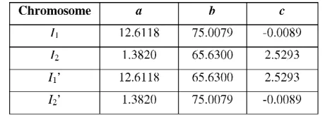
The real values of the model parameters for each chromosome in this crossover process are tabulated in Table 2. Equations 15, 16 and 17 are used to decode the binary number to real numbers.
6. Mutation
The final operation is mutation. This operation will change 1 to 0 and vice versa using the small mutation probability. In this study, only 1% of total bit (55 x N) of population undergo mutation. Assume that the 25thgene (or bit) of the chromosome
I1 is selected for a mutation. A simple example given below shows how the mutation takes place in the single chromosome: c= -0.001 + decimal number x 5-(-0.001)
216-1
Table 1: Binary, decimal and real number for a, b and c
Table 3 presents the real values of the model parameters for each chromosome in this process.
The entire process was repeated until the specified maximum number of generations was attained. After 200 generations (maximum number of generation), each chromosome was then mapped to the real values using lower and upper bounds specified earlier. It is important to note that the GA is a stochastic procedure, and should be run multiple times before a solution is accepted [35].
5.0 RESULTS AND DISCUSSIONS
The main procedure of an optimisation approach is to search the best parameters, which minimises the error functions. The Gauss-Newton method and genetic algorithms were employed, analysed and compared in this study.
5.1 GAUSS-NEWTON METHOD
The Gauss-Newton of least squares method was used to determine the optimum values of a, b and c. This method minimises the residuals (the difference between calculated and observed values). Table 1 summarises the estimated values a, b and cobtained using the Gauss-Newton method. It can be seen clearly from the table that the estimated value of a ranges from 0.09 to 45 561, the estimated value of b ranges from 25 to 459 and the estimated value of c ranges from –0.003 to 3.5. The study by [13] assumed that c could be neglected since its value is very small compared with x. However, in this study, the value of c is appreciable and its value (in some case) is significant compared with the value of x. Therefore, ccannot be ignored.
When using this type of optimisation method, tremendous guessing of the initial parameters was involved in order to ensure convergence and to avoid complex solutions. Thus, for each operating conditions, many runs were required to estimate the model parameters and only the one that produces the best predictive accuracy is presented here. As can been seen in Table 4, some of the estimated values (such as a equals to 28123/min or 45561/min) are large compared with the reported values by [13] and it seems that those values are not reasonable kinetic parameters for the process under study. Based on our review, the largest value for the reaction rate of a similar process is only 633/min [36].
Comparison between the predicted (solid line) and the experimental values of glucose concentration at different initial dry solid and enzyme concentrations are shown in Figures 2a to 5a. These figures indicate that considerable discrepancy between the predictions and measurements is noticeable
towards the end of the reaction. One possible explanation for the poor agreement between the model and the experimental values at the end of the reaction is the failure of the model to account for end-product inhibition. It is possible that the model failed to describe the reaction profile due to insignificant number of model parameters.
In many cases, the model that used estimated parameters by the Gauss-Newton method is able to achieve prediction performance with less than 5% error (refer to Table 1) and the overall predictive error is 3.16%. The weakness of the Gauss-Newton method for solving the coefficients of the nonlinear equation is that good initial values of a0, b0and c0are needed to
ensure convergence. In addition, incorrect starting values of the coefficients led to a solution of complex numbers that has no physical meaning in the process under study.
5.2 GENETIC ALGORITHM
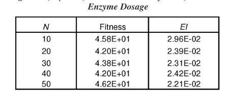
The influence of the user defined parameters (population size, mutation rate and crossover rate) of the genetic algorithm was studied. The GA performance was evaluated based on the fitness and error index values. In the current experiments, the population size ranged from 10 to 50, the crossover rate ranged from 0.6 to 1.0, and the mutation rate was varied from 0.001 to 0.05. These parameter settings have been used in a number of implementations of genetic algorithms. The results are depicted in Tables 5, 6 and 7. Examination of the results in Tables 5, 6 and 7 shows that there is no obvious relationship between the user defined parameters and the GA performance. In addition, the effects of those parameters on the GA performance are insignificant. The predictive performance (EI) is found not to be very sensitive on the GA control parameters as compared with the initial parameters of Gauss-Newton method. However, it is found that for large values of population size, an inordinate amount of time will be required to perform all the evaluation. This is in agreement with the work done by [21, 24].
Table 3: Real values of the model parameters in the mutation process
Table 4: Parameter estimation using Gauss-Newton method
Table 5: The effect of population size N on the GA performance. Pm= 0.01, Pc= 0.6, 10 %w/v Initial Dry Solid, 0.7 L/ton
The following parameters of the genetic algorithm were used to determine the model parameters for the rest of the experimental data: probability for cross over (Pc= 0.6), probability for mutation
(Pm= 0.01), and number of chromosomes in each population (N=
30). Table 8 presents values of the coefficients estimated by the application of the GA method. The estimated value of a ranges from 0.0045 to 21.40, the estimated value of branges from 14.80 to 148.94 and the estimated value of cranges from 0.0085 to 3.81. Compared with the Gauss-Newton approach, the GA method requires no initial guesses of the coefficients and therefore only few simulations are needed. Due to the global search capability of GA, the GA method is able to give viable values of the estimated parameters. This clearly demonstrates the effectiveness of the GA method as compared with the Gauss-Newton method for parameter estimation. Furthermore, large values of a estimated using the Gauss-Newton method can be avoided by constraining the range of a.
The resulting profiles of glucose concentration are shown in Figures 2 to 5. These figures compare the predicted output based on the model parameters estimated using GA and those using the Gauss-Newton method.
There exit a little difference between the measured output and the predicted output at the end of the reaction time for both models as illustrated in Figures 2 to 5. The reason for this phenomenon was due to the failure of the empirical model to account for end-product inhibition at longer reaction time. It seems that the model is adequate only for shorter reaction time as shown in the work of [13].
Table 6: The effect of mutation rate Pmon the GA performance.
N=30, Pc= 0.6, 10 %w/v Initial Dry Solid, 0.7 L/ton Enzyme Dosage
Table 7: The effect of crossover rate on the predictive performance. N=30, Pm= 0.01, 10 %w/v Initial Dry Solid,
0.7 L/ton Enzyme Dosage
Table 8: Parameter estimation results using genetic algorithm. N = 30, Pm= 0.01, Pc= 0.6
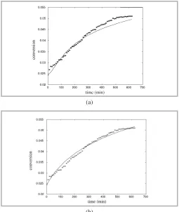
(a)
(b)
Figure 2: Prediction curve using (a) Gauss Newton, EI = 0.0367 (b) GA, EI = 0.0229 Initial dry solid = 20%w/v, Enzyme dosage = 0.95 L/ton, x = experimental data, ___ = simulated curve
(a)
(b)
The overall predictive error obtained using GA approach (2.67%) is slightly better than that obtained by the Gauss-Newton method (3.16%). Figures 2 and 4 clearly indicate that the GA method is able to produce better prediction curves. Even though, Figures 3 and 5 shows comparable curves are obtained using either GA or the Gauss-Newton method, the estimated values resulted from both methods are significantly different (refer to Table 1 and 2). Obviously, in real application, reasonable estimated values are more appreciated for describing the process under consideration. Therefore, the estimated values resulted from genetic algorithm are more acceptable.
6.0 CONCLUSIONS
In this work, the Gauss-Newton of least square technique and the Genetic Algorithm method were utilised for parameter estimation of the empirical model of tapioca starch hydrolysis process. The performances of both parameter estimation approaches were evaluated and compared based on the error index values and the graphical plots.
The Gauss-Newton algorithm was found advantageous when a good initial parameter estimate was provided. However, the search for suitable starting points proved to be difficult. If the initial value lies within the environment of a local optimum, then this search method converges at this optimum. In addition, the Gauss-Newton algorithm may also result in complex values of the model parameters that have no physical meaning. Frequently, many trials were necessary to obtain a suitable starting value to avoid complex solutions.
The impact of user defined parameters of the GA was not very sensitive as compared with the influence of initial parameters of the Gauss-Newton method on the predictive performance. Compared with the Gauss-Newton technique, GA provided a higher potential for finding the global solution, even though the range to be considered for each parameter was wider. Thus, few simulations were required. Furthermore, no guessing of initial values was required and reasonable solutions were able to be obtained when using the GA optimisation method. The model using the parameter values estimated by the GA followed the glucose concentration profile quite well and in fact gave a much higher value of overall predictive performance than the Gauss-Newton method. In summary, the GA has been successfully applied to perform nonlinear kinetic parameter estimation of tapioca starch hydrolysis process and is able to produce better results than those of the Gauss-Newton Method. In addition, the GA approach has solved the problem of guessing initial parameters required by the Gauss-Newton method.
ACKNOWLEDGEMENTS
This work was supported by the Ministry of Science Technology and Environment Fund, Malaysia. ■
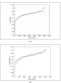
(a)
(b)
Figure 4: Prediction curve using (a) Gauss-Newton EI = 0.0315 (b) GA, EI = 0.0234. Initial dry solid = 10%w/v, Enzyme dosage = 1.2 L/ton, x = experimental data, ___ = simulated curve
(a)
(b)
REFERENCES
[1] T. R Swanson, J. O. Carroll, R. A Britto, and D. J. Duhart, “Development and Field Confirmation of a Mathematical Model for Amyloglucosidase/Pullulanase Saccharification”. Starch/starke, Vol. 38, pp. 382-387, 1986.
[2] D Paolucci-Jeanjean,. M-P Belleville, N Zakhia, and G. M Rios, “Kinetics of Cassava Starch Hydrolysis with Termamyl Enzyme”. Biotechnology and Bioengineering, Vol. 68, pp. 71-77, 2000.
[3] J Bryjak, K Murlikiewicz,. I, Zbicinski, and J Stawczyk, “Application of Artificial Neural Networks to Modelling of Starch Hydrolysis by Glucoamylase”. Bioprocess Engineering, Vol. 23, pp. 351-357, 2000.
[4] L. Davis, Handbook on Genetic Algorithms, New York: Van Nostrand Reinhold, 1991.
[5] D. E Goldberg, Genetic Algorithms in Search, Optimization and Machine Learning. Reading, New York: Addison-Wesley, 1989.
[6] J. R Lobry, and J. P Flandrois, “Comparison of Estimates of Monod’s Growth Model Parameters from the Same Data Set”. Binary, Vol. 3, pp. 20-23, 1991.
[7] M. Ranganath, S. Renganathan, and C. Gokulnath, “Identification of Bioprocesses using Genetic Algorithm”. Bioprocess Engineering. Vol. 21, pp. 123-127, 1999.
[8] M. Gen, and R. Cheng. Genetic Algorithms and
Engineering Design. New York: Wiley Interscience, 1997.
[9] A. Eftaxias, J. Font, A. Fortuny, A. Fabregat, and F. Stuber,. “Nonlinear Kinetic Parameter Estimation Using Simulated Annealing” Computers and Chemical Engineering. Vol. 26, pp. 1725-1733, 2002
[10] R. C. L. Marteijn, O. Jurrius, J. Dhont, C. D. Gooijer, J. Tramper, and D. E. Martens. “Optimization of a Feed Medium for Fed-batch Culture of Insect Cells Using a Genetic Algorithm”. Biotechnology and Bioengineering. Vol. 81, No. 3: pp. 269-278, 2003.
[11] J.-G Na, Y. K. Chang, B. H. Chung, and H.C. Lim, “Adaptive Optimization of Fed-batch Culture of Yeast by Using Genetic Algorithms”. Bioprocess and Biosystems Engineering. Vol. 24, pp. 299-308, 2002.
[12] L. J. Park, C. H. Park, C. Park, and T. Lee, “Application of Genetic Algorithms to Parameter Estimation of Bioprocesses”. Medical and Biological Engineering and Computing. Vol. 35, No. 1, pp. 47-49, 1997.
[13] P. Gonzalez-Tello, F. Camacho, E. Jurado, and E. M. Guadix, “A Simple Method for Obtaining Kinetic Equations to Describe the Enzymatic Hydrolysis of Biopolymers”. Journal of Chemical Technology and Biotechnology. Vol. 67, pp. 286-290, 1996.
[14] C. Akerberg, G. Zacchi, N. Torto, and L. Gorton, “A Kinetic Model for Enzymatic Wheat Starch
Saccharification”. Journal of Chemical Technology and Biotechnology. Vol. 75, pp. 306-314, 2000.
[15] C. S. James, Analytical Chemistry of Food. UK: Blackie Academics Professional, 1995
[16] L. Ljung, System Identification: Theory for the User. New Jersey: Prentice Hall, 1987.
[17] R. I. Jennrich,. An Introduction to Computational Statistics: Regression Analysis. New Jersey: Prentice Hall, 1995
[18] M. Matsumura, J. Hirata, S. Ishii, and J. Kobayashi, “Kinetics of Saccharification of Raw Starch by Glucoamylase”. J Chem. Tech. Biotechnol. Vol. 42, pp. 51-67. 1988.
[19] J. H. Holland, Adaption In Natural and Artificial Systems. University of Michigan Press, Ann Arbor, 1975.
[20] M. Negnevitsky,. Artificial Intelligence. A Guide to Intelligent Systems. Pearson Education Limited, UK, 2001.
[21] R. Moros, H. Kalies, H. G. Rex, and S. T. Schaffarczyk, “A Genetic Algorithm for Generating Initial Parameter Estimations for Kinetic Models of Catalytic Processes”. Computers Chemical Engineering. Vol. 20, No. 10, pp. 1257-1270, 1996.
[22] M. Mitchell, An Introduction to Genetic Algorithms. MIT Press: Cambridge, MA , 1996.
[23] T-Y Park, and G. F. Froment, “Hybrid Genetic
Algorithm for the Estimation of Parameters in Detailed Kinetic Models”. Computers Chemical Engineering. Vol. 22, pp. S103-110, 1998.
[24] J. G. Digalakis, and K. G. Margaritis, “An Experimental Study of Benchmarking Functions for Genetic
Algorithms”. IEEE International Conference on Systems, Man and Cybernetics, pp.3810-3815, 2000.
[25] H. Moriyama, and K. Shimizu, “On-line Optimization of Culture Temperature for Ethanol Fermentation Using a Genetic Algorithm”. Journal of Chemical Technology and Biotechnology. Vol. 66, pp 217-222, 1996.
[27] J. J. Grefenstette, “Optimisation of Control Parameters for Genetic Algorithms”. IEEE Transaction System Man. Cybernet. SMC-16: 122-128, 1986.
[28] Z Shi, and H. Aoyama, “Estimation of the Exponential Autoregressive Time Series Model by Using the Genetic Algorithm”. Journal of Sound and Vibration. Vol. 205, No. 3, pp. 309-321, 1997.
[29] D. Weuster-Botz, V. Pramatarova, G. Spassov, and C Wandrey, “Use of a Genetic Algorithm in the Development of a Synthetic Growth Medium for Arthrobacter simplex with High Hydrocortisone ∆’-Dehydrogenase Activity”. Journal of Chemical Technology and Biotechnology. Vol. 64, pp. 386-392, 1995.
[30] L Yao, and W. A. Sethares, “Nonlinear Parameter Estimation via the Genetic Algorithm”. IEEE
Transactions on Signal Processing. Vol. 42, No.4, pp. 927-935, 1994.
[31] P Angelov, and R. Guthke, “A Genetic-algorithm-based Approach to Optimization of Bioprocess Described by Fuzzy Rules”. Bioprocess Engineering. Vol. 16, pp. 299-303, 1997.
[32] S Rivera, Neural Networks and Micro-Genetic Algorithms for State Estimation and Optimization of Bioprocesses.Colorado State University, US: Doctoral Thesis, 1992.
[33] A. K. Y. Yee, A. K. Ray, and G. P. Rangaiah,
“Multiobjective Optimization of an Industrial Styrene Reactor”. Computers and Chemical Engineering. Vol. 27, pp 111-130, 2003.
[34] D. Sarkar, and J. M. Modak, “Optimization of Fed-batch Bioreactors using Genetic Algorithms”. Chemical Engineering Science. Vol. 58, pp. 2283-2296, 2003.
[35] R.J. Pinchuk, W. A. Brown, S. M. Hughes, and D. G. Cooper, “Modeling of Biological Processes Using Self-Cycling Fermentation and Genetic Algorithms”. Biotechnology and Bioengineering. Vol. 67, No.1, pp. 19-24, 2000.
[36] Z. L. Nikolov, M.M. Meagher, and P. J. Reilly,
“Kinetics, Equilibia, and Modeling of the Formation of Oligosaccharides form D-glucose with Aspergillus Niger Glucoamylase I and II”. Biotechnology and Bioengineering. Vol. 34, pp. 694-704, 1989.
PROFILE
Roslina Rashid
Faculty of Chemical & Natural Resources Engineering, University Teknologi Malaysia, 81310 Skudai, Malaysia.
Nor Aishah Saidin Amin
Faculty of Chemical & Natural Resources Engineering, University Teknologi Malaysia, 81310 Skudai, Malaysia.
Hishamuddin Jamaluddin