Abstract
BAEK, CHANGSEOK. Determining Visibility Distance of Signs Installed on the Roadside Using Videologs. (Under the direction of Dr. Joseph E. Hummer.)
Biography
Acknowledgments
Contents
List of Figures v
List of Tables vii
Chapter 1: Introduction 1
1.1 Background ··· 1
1.2 Objectives and Scope ··· 2
Chapter 2: Literature Review 6 2.1 Surveying Signs and Obstructions ··· 6
2.2 Sign Visibility Distance ··· 9
Chapter 3: Methodology 13 3.1 Introduction to 3M Transportation Asset Management Services ··· 13
3.2 Assumptions Regarding the Determination of Visible Distance of Signs and Obstructions on the Videologs ··· 14
3.3 How to Calculate Sight Distance on 3M TAMS ··· 14
3.4 The Spreadsheet Columns··· 17
3.5 Signs Selected··· 19
Chapter 4: Analysis of Sign Data from Videologs 20 4.1 Sign Survey Results··· 20
4.2 Visibility Distances for Obstructed Signs ··· 24
4.3 Visibility Distances for Unobstructed Signs ··· 31
4.4 Statistical Analysis of the Data Set ··· 40
Chapter 5: Conclusions and Recommendations 46
5.1 Conclusions ··· 46
5.2 Recommendations ··· 47
List of Figures
Figure 1.1 The horizontal alignment for the fringe two-lane highway sampled ··· 4
Figure 1.2 The horizontal alignment for freeway ··· 5
Figure 2.1 Connecticut DOT’s data collection vans ··· 7
Figure 2.2 Visibility of three sizes of sign with restricted and unrestricted sight distance ··· 10
Figure 3.1 3M’s van with camera and software ··· 13
Figure 3.2 The caption of an image on the videolog ··· 15
Figure 3.3 Typical image in which a sign becomes visible on the videolog ··· 16
Figure 3.4 Typical image with a hill obstruction ··· 17
Figure 4.1 Percent obstructed by sign location ··· 22
Figure 4.2 Percent obstructed by lateral offset ··· 22
Figure 4.3 Cumulative distributions of visibility distance in the fringe area ··· 25
Figure 4.4 Cumulative distributions of visibility distance in the rural area ··· 25
Figure 4.5 Cumulative distributions of visibility distance in the urban area ··· 25
Figure 4.6 Cumulative distributions of visibility distance on the freeway ··· 26
Figure 4.7 Cumulative distributions of visibility distance for obstructed sings by road type ··· 27
Figure 4.8 Cumulative distributions of visibility distance for obstructed signs by sign type ··· 28
Figure 4.9 Cumulative distributions of visibility distance for obstructed signs by offset ··· 28
Figure 4.12 Visibility distances for signs obstructed by hills ··· 30
Figure 4.13 Visibility distances for signs obstructed by objects ··· 30
Figure 4.14 Visibility distances for unobstructed signs in the fringe area ··· 32
Figure 4.15 Visibility distances for unobstructed signs in the rural area ··· 32
Figure 4.16 Visibility distances for unobstructed signs in the urban area ··· 32
Figure 4.17 Visibility distances for unobstructed signs on the freeway ··· 33
Figure 4.18 Cumulative distributions of visibility distance for unobstructed signs by sign size ··· 33
Figure 4.19 Cumulative distributions of visibility distance for unobstructed signs by road type ··· 34
Figure 4.20 Visibility distances for unobstructed warning signs ··· 35
Figure 4.21 Visibility distances for unobstructed regulatory signs ··· 35
Figure 4.22 Visibility distances for unobstructed guide signs ··· 35
Figure 4.23 Cumulative distributions by sign type ··· 36
Figure 4.24 Visibility distances for unobstructed speed limit signs ··· 37
Figure 4.25 Visibility distances for unobstructed stop signs ··· 37
Figure 4.26 Visibility distances for unobstructed curve warning signs ··· 38
Figure 4.27 Visibility distances for unobstructed no passing zone signs ··· 38
Figure 4.28 Visibility distances for unobstructed street name signs ··· 38
List of Tables
Table 2.1 Directional Guide-Sign view interferences ··· 8
Table 2.2 Average luminance of sign surroundings, at 1500 ft distance ··· 11
Table 3.1 Example of developed spreadsheet columns ··· 18
Table 4.1 Total number of sings by road type and sign type ··· 20
Table 4.2 Number and percentage of obstructed signs by road type ··· 21
Table 4.3 Number and percentage of obstructed signs by sign type ··· 21
Table 4.4 Survey of obstructions ··· 23
Table 4.5 Breakdown of objects obstructing signs ··· 24
Table 4.6 Breakdown of number of obstructing signs below 400 feet of visibility distance ··· 26
Table 4.7 Number of unobstructed signs by road type and sign size ··· 31
Table 4.8 ANOVA table for obstructed signs ··· 41
Table 4.9 Tukey-Kramer multiple comparisons for type of obstruction ··· 41
Table 4.10 Tukey-Kramer multiple comparisons for road type ··· 41
Table 4.11 Tukey-Kramer multiple comparisons for sign size ··· 41
Table 4.12 ANOVA table for obstructed signs for road type ··· 42
Table 4.13 Number of unobstructed signs by category ··· 43
Table 4.14 Tukey-Kramer multiple comparisons of unobstructed visibility distance for sign color ··· 43
Table 4.15 Tukey-Kramer multiple comparisons unobstructed visibility distance for sign size ··· 44
Table 4.16 The adjusted means of color and size combination for unobstructed signs ··· 44
Chapter 1: Introduction
1.1 Background
Drivers often become complacent as they travel familiar routes, and they are less likely to notice approaching signs. However, along an unfamiliar route, drivers are dependent upon signs as a source of information to help them safely navigate their vehicles. The purpose of traffic signs is to provide information for the orderly movement that guides all road users as to direction, regulations and warnings. This information is also strongly related to highway safety. Therefore, the Manual on Uniform Traffic Control Devices (MUTCD)(1), the nationally recognized authority on traffic control devices for all public roads in the U.S., recommends that every traffic control device meet these five basic requirements:
A. Fulfill a need; B. Command attention;
C. Convey a clear, simple meaning; D. Command respect from road users; and E. Give adequate time for proper response.
Many engineers and designers who deal with traffic signs refer to the MUTCD, but it does not provide standards or guidance for all aspects of sign design because it cannot consider every situation that may meet the designer or traffic engineer. On sign visibility, for example, the Manual simply recommends that a sign be located in the road user’s view for a long time to maximize safety and efficiency.
time for proper response. If signs are obscured or blocked for some reason, drivers may not be ready to respond to these signs.
1.2 Objectives and Scope
Objectives
A driver may be able to view sign sheetings from a long distance with no sight obstruction. However, there are many cases in which the driver’s line of sight is blocked by obstructions, such as trees, hills, curves, and other signs. These obstructions may reduce a visibility distance from where a sign becomes visible to a sign itself. If the visibility distance is too short drivers may find it more difficult to perform thorough maneuvers such as merging, traveling through reverse curves, and navigating one-way streets.
The 3M Company (3M) currently has a collection of videologs recorded along representative samples of U.S. highway routes, taken from the driver’s perspective. Images from these databases are suitable for determining the distance at which installed signs become visible to drivers and identifying obstructions that block the line of sight. The visibility distance will be first potential information to drivers. The main objectives of this project, therefore, are to determine the distribution of the visibility distance for signs and to identify reasons for being obscured. This distribution of the visibility is to be the “supply” of visibility. The “demand” of visibility will be needed from other research efforts on motorist’s needs for information.
• Sign designers may be able to design new sheetings that are better suited to real highway environments and geometries. Sign designers may be able to customize sign characteristics by road type, sign type, sign size and sign color.
• Highway engineers or agencies will be better informed as they set guidelines for avoiding visibility problem areas that exist on current highways.
• Finding the reasons for obstructions on a representative sample of U.S. highways will guide sign placement in order to avoid blocked views.
Scope
Signs of interest in this research include all warning signs, important regulatory signs, and important guide signs. Warning signs include the right, left and reverse curve signs; the chevron alignment sign; the stop ahead sign; the crossing road sign; the no passing zone sign; and the school advance sign. The important regulatory signs include the stop sign, the speed limit sign, the no left turn sign, the do not enter sign, the no turn on red sign, and the one-way sign. Important guide signs include the street name sign, the general information sign, the state route marker, the junction marker, the directional arrow sign, and the county road marker. The method of choosing signs for observation requires sampling to maintain relatively standard conditions so that, for example, we measured signs on cloudy or sunny days but did not measure signs in dark or directly backlit conditions.
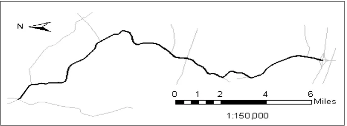
1) A typical two-lane state highway in a developing fringe area of Maryland where 3M collected videologs that is characteristic of many such fringe roads generally located on the edges of urban areas. Although the geometric characteristics of a fringe road are generally closer to rural design, it nonetheless carries significant traffic volumes and provides direct access to surrounding business. There is only one road in this environment, from which 3M collected videologs in both directions. Figure 1-1 shows its horizontal alignment; it has several sharp curves over its 17 miles.
Figure 1-1: The horizontal alignment for the fringe two-lane highway sampled.
2) The two-lane roads in a rural Minnesota county that connect farms, homes, and small towns. Among the 200 miles of roads surveyed by 3M in the county, several roads were selected at random for study in this research. Most of the roads selected were county-maintained; a few roads were unpaved. 3M collected videologs in this county during the winter season, with some roads having snow in the background of the picture.
streets, and one-way streets were selected at random (after a check to discard short segments from the sample) and most of the sampled streets were city-maintained.
4) 3M also collected videologs on a 6-lane interstate highway in the suburbs of a mid-sized urban area in the foothills of the Appalachians. Many guide signs were located overhead in this sample. Both directions of the freeway were used. Figure 1-2 shows the horizontal alignment of the 17 miles of the freeway in the sample, which included interchanges.
Figure 1-2: The horizontal alignment for freeway.
Organization of Thesis
Chapter 2: Literature Review
This chapter reviews the literature on surveying signs in real environmental conditions and on the effects of sign visibility distance. The review will show that a method using photologs or videologs for surveying sign visibility distance has some precedent and that reasons for obstruction have been studied in previous research.
2.1 Surveying Signs and Obstructions
Surveying signs to determine visibility distance and to classify obstructions is easily carried out in the field, but it is expensive, potentially dangerous and slow. Through the use of advanced technology, such as huge digital storage capabilities and the Global Positioning System (GPS), digital images can be recorded from the driver’s viewpoint for later analysis. While this method has double the steps of a purely manual effort (to observe samples in the field and then perform the laboratory work), it is nevertheless useful for performing accurate measurements of sign visibility distance and making a percentage statement of obstruction reasons and is faster, less expensive and more adaptable for surveying thousands of signs than a manual observation method (2). King and Lunenfeld (3), for example, used videotapes of approaches to signs for analyzing a legibility distance formula that includes the number of information elements on a sign.
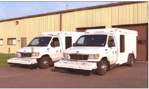
Richard Hanley, who helped compile the Connecticut DOT inventory, estimated that a completed VSIS would yield initial savings of 60,000 miles of travel, 40,000 person-hours and more than $800,000 over a statewide field inventory of highway signs. In addition to such savings, there is a substantial reduction in the hazard to survey crews. However Hanley also mentioned problems surrounding the Photolog data, such as poor image resolution when transferring images from film to videodisc and mismatched mileage readings using a vehicle-mounted fifth-wheel device to record mileages.
Figure 2-1: Connecticut DOT’s data collection vans (4).
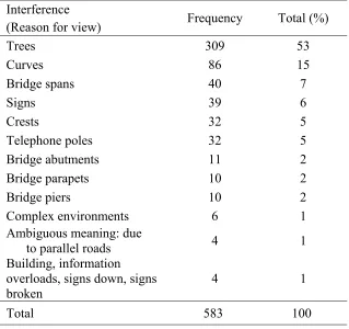
accounted for 5%, curves and crests for 20%. Table 2-1 shows the distribution of obstructions by number and percentage.
Table 2-1: Directional Guide-Sign view interferences (2). Interference
(Reason for view) Frequency Total (%)
Trees 309 53
Curves 86 15
Bridge spans 40 7
Signs 39 6
Crests 32 5
Telephone poles 32 5
Bridge abutments 11 2
Bridge parapets 10 2
Bridge piers 10 2
Complex environments 6 1
Ambiguous meaning: due
to parallel roads 4 1
Building, information overloads, signs down, signs
broken 4 1
Total 583 100
2.2 Sign Visibility Distance
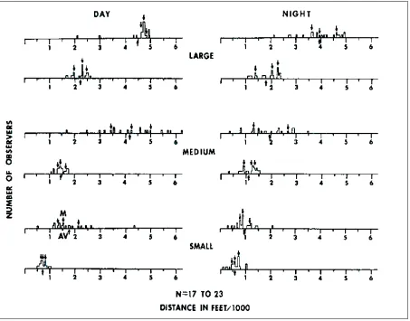
There are two main areas of sign visibility evident in the literature. One is sign detectability (visibility, i.e. the capability to discern that there is a sign present) and the other is sign legibility (the capability of being read). The visibility distance is usually longer than the legibility distance except in cases where the line of sight is blocked. Both are interdependent; a sign cannot be read if it is not visible. However, Kuhn et al. (7) state that for sign design and placement, the characteristics that affect legibility and detection differ enough qualitatively to warrant separate consideration.
Figure 2-2: Visibility of three sizes of sign with restricted and unrestricted sight distance (8). (Arrows indicate 25 and 50 percentile and arithmetic mean)
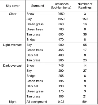
Table 2-2: Average luminance of sign surroundings, at 1500 ft distance (10).
Sky cover Surround (foot-lamberts)Luminance Number of Readings
Clear Snow 2650 3
Sky 1950 150
Green grass 860 16
Green trees 700 6
Tan grass 600 36
Bridge 470 8
Light overcast Sky 900 65
Green trees 455 17
Dark hill 400 8
Tan grass 285 23
Dark overcast Snow 745 14
Sky 290 27
Bridge 255 6
Green trees 195 8
Dark hill 190 9
Green grass 175 3
Tan grass 106 21
Night All background 0.02 504
effective color of sign background among the colors black, light gray and yellow. Mace et al. (14) found black/white signs to provide particularly poorer conspicuity than black/orange and white/green signs. Moreover, Mace and Pollack (12) stated that sign conspicuity increases with increased sign luminance.
Regarding size and shape, Jenkins and Cole (15) conducted a study that provides corroborative data that size is a key factor in sign detection. They concluded that sign sizes between 15 in. and 35 in. are sufficient to guarantee visibility and that if signs this size or bigger are not visible then the problem is due to external contrast or surround complexity.
Chapter summary
Chapter 3: Methodology
3.1 Introduction to 3M Transportation Asset Management Services
3.2 Assumptions Regarding the Determination of Visible Distance of Signs and
Obstructions on the Videologs
Presumably, drivers cannot recognize signs beyond their individual visibility range; furthermore, a sign’s appearance precedes eventual driver recognition. There are two possible scenarios for drivers approaching a sign. The first case is that there is no significant impediment blocking the driver’s line of sight. The second case involves a significant obstruction that may block the driver’s line of sight or significantly influence the sign’s appearance. Once an initial obstruction occurs, it is easy to determine the visibility distance: it is from where the obstruction no long blocks the sight of the sign to the sign itself. A measure for “no longer obstruction” is half of the sign is visible. In the absence of a tangible obstruction, however, determining a visibility distance is more difficult because the limiting factor is the quality of the image. This method may not consider a sign’s luminance, contrast, shape and border. Thus, in this study we recorded the visibility distance of a sign with no obstruction as the distance between when the sign first appeared as a “dot” on our screen or distinguished itself from its surroundings to the sign itself.
3.3 How to Calculate Sight Distance on 3M TAMS
where the sign first becomes visible to drivers. Because a DMI reading was recorded along the road, this distance is along the roadway, not on a straight line.
The following explains the procedure I used to find visibility distance from these images on my 17-inch computer monitor.
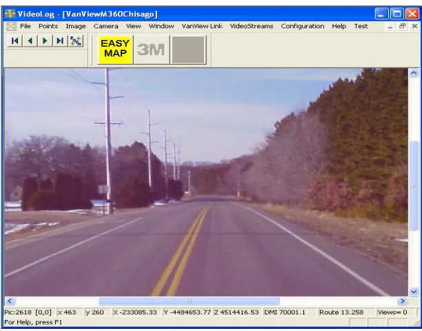
1. Find an image in which a sign is immediately ahead on the 3M TAMS software, as shown in Figure 3-2.
Figure 3-2: The caption of an image on the videolog. 2. Check the DMI reading, sign ID number and an image ID number.
4. Continue to move away from the sign until the sign became invisible on the image or until the sign resembles a dot as shown in Figure 3-3.
Figure 3-3: Typical image in which a sign becomes visible on the videolog.
5. Check the DMI reading of the image at which the sign become visible.
Figure 3-4: Typical caption of an image with a hill obstruction. 7. Calculate the visibility distance from the two DMI readings:
Visibility distance = DMI from step 1 – DMI from step 4 or 5
3.4. The Spreadsheet Columns
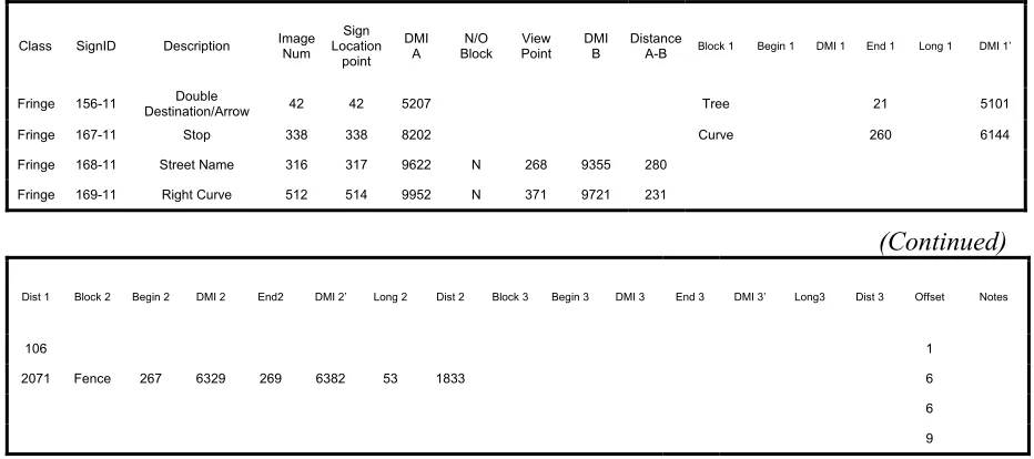
Table 3-1 shows an example of the spreadsheet I used to record visibility distance data. The definitions of the column headings include:
• SignID: An identified number of a sign
• ImageNum: An orderly number of the picture stream on the Videologs • SignLocationPoint: A number of image in which a sign is immediately ahead • DMI A: Actual unit of distance converted from ‘SignLocationPoint’ (ft) • N/O Block: ‘N’ means there is no obstruction in the sight of line
• ViewPoint: The image number where the sign becomes visible • DMI B: Actual unit of distance converted from ‘ViewPoint’ (ft)
• DMI 1: Actual unit of distance converted from ‘Begin 1’ (ft)
• End 1: The number of the image in which a sign becomes visible after the obstruction first encountered
• Long1: How long a sign is obscured by the first obstruction (ft) • DMI 1’: Actual unit of distance converted from ‘End 1’ (ft)
• Dist 1: Visibility distance from Step 7, in the case of the first obstruction • Block 2: The type of obstruction encountered second
• Begin 2: The number of the image in which a sign become visible after the obstruction encountered second
• DMI 2: Actual unit of distance converted from ‘Begin 2’ (ft)
• End 2: The number of the image in which a sign becomes visible after the obstruction encountered second
• Long 2: How long a sign is obscured by the second obstruction (ft) • DMI 2’: Actual unit of distance converted from ‘End 2’ (ft)
• Dist 2: Visibility distance from Step 7, in the case of the second obstruction • Block 3, Begin 3, DMI 3, End 3, DMI 3’, Long 3 and Dist 3: The case of
obstruction encountered third
• Offset: Measured from the right edge of paved road to the left edge of the signs (ft). Table 3-1: Example of developed spreadsheet columns.
Class SignID Description Image Num LocationSign point
DMI
A Block N/O Point View DMI B DistanceA-B Block 1 Begin 1 DMI 1 End 1 Long 1 DMI 1’
Fringe 156-11 Destination/Arrow Double 42 42 5207 Tree 21 5101
Fringe 167-11 Stop 338 338 8202 Curve 260 6144
Fringe 168-11 Street Name 316 317 9622 N 268 9355 280
Fringe 169-11 Right Curve 512 514 9952 N 371 9721 231
(Continued)
Dist 1 Block 2 Begin 2 DMI 2 End2 DMI 2’ Long 2 Dist 2 Block 3 Begin 3 DMI 3 End 3 DMI 3’ Long3 Dist 3 Offset Notes
106 1
2071 Fence 267 6329 269 6382 53 1833 6
6
3.5. Signs Selected
The fringe area, the rural area and the freeway had a total of 3601 signs in the recorded area, but 2260 signs were actually used in determining visibility distances. The signs ignored during data collection were signs for another street (which were approximately 50 percent of those ignored) parking signs, object markers, and signs with images below somewhat standard conditions such as backlit and glare, etc. It was difficult to find the number of total signs on the urban roads because many signs were discarded from the set of disjointed streets.
Chapter summary
Chapter 4: Analysis of Sign Data from Videologs
This chapter discusses the results of the visibility distance data collection effect by road type, sign type, color, size, location and lateral offset. Sections 4.1, 4.2 and 4.3 provide single variable tabulations and breakdowns of the results while section 4.4 provides a more sophisticated statistical analysis of the data.
4.1. Sign Survey Results
Table 4-1 shows the number of signs on which I made a visibility distance measurement, classified by the four highway system types and four main sign types. A total of 3142 signs was observed, of which 1261 (40.1%) were in the rural area, 882 (28.1%) were in the urban area, 432 (13.7%) were in the fringe area and 567 (18.0%) were on the freeway. For sign types, there were 967 (30.8%) warning signs, 769 (24.5%) regulatory signs and 1211 (38.5%) guide signs. There were 195 (6.2%) signs that were categorized as others; these include the individual state’s own style signs, clearance markers, a left lane no truck sign in the freeway, etc. Guide signs were the most commonly-measured signs on the fringe road and freeway, warning signs were the most commonly-measured signs on the rural roads, and regulatory signs were the most commonly-measured on the urban streets.
Table 4-1: Total number of signs by road type and sign type. Road Type
Sign type
Fringe Rural Urban Freeway Total
Warning 153 621 138 55 967
Regulatory 82 164 499 24 769
Guide 271 446 236 258 1211
There were 2497 signs (79.1%) that were obscured for some reason among the total of 3142 signs. Table 4-2 shows that 660 signs (20.9%) were unobstructed. Note that 15 signs included among the 660 signs were blocked later after initially being unobstructed.
At the extremes, 67.8% of the signs in the rural area and 96.9% percent of the signs in the urban area had a blocked view, as shown in Table 4-2. Regulatory signs had the highest percentage (88.3%) of blocked views. Warning signs had the highest percentage (29.8%) of unobstructed views.
Table 4-2: Number and percentage of obstructed signs by road type.
Fringe Rural Urban Freeway Total
26.0% 32.2% 3.1% 17.4% 20.9% Unobstructed
view 149 409 27 75 660
74.0% 67.8% 96.9% 82.6% 79.1%
Blocked view 423 862 855 357 2497
Table 4-3: Number and percentage of obstructed signs by sign type.
Warning Regulatory Guide Others Total
29.8% 11.7% 18.9% 25.3% 20.9% Unobstructed
view 290 90 230 50 660
70.2% 88.3% 81.1% 74.7% 79.1%
Blocked view 683 681 985 148 2497
even in the case of an obstructed view. The visibility distance of obstructed signs is described in Section 4.2.
89.2 67.9 80.2 0 20 40 60 80 100
Overhead Left shoulder Right shoulder
Pe rc en t o bs tr uc te d Obstructed Unobstructed
Figure 4-1: Percent obstructed by sign location.
I combined the lateral offset data into three categories: 1 to 3 feet, 4 to 8 feet, and more than 9 feet. In the case of lateral offset, the 4 to 8 feet category has the smaller percentage of obstruction, at 74.9%.
80.8 74.9 77.4
0 20 40 60 80 100 1~3 feet Lateral offset 4~8 feet Lateral offset
9~ feet Lateral offset P er cen t o bs tr uct ed Obstructed Unobstructed
Figure 4-2: Percent obstructed by lateral offset.
obstruction. There were 122 signs in the sample blocked a second time and 12 signs blocked a third time. Once these blockages happened, the average of blocked distances was 270 feet.
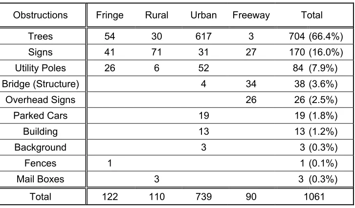
A total of 42.2% of blocked views are related to curves, and 15.7% are related to hills. This indicates that the effectiveness of many signs is reduced by the geometric design of the highway itself. Among the road types, the urban area had the highest number of signs blocked by objects, 85.8%. The highest percentage for signs blocked by hills was in the rural area, 28.2%.
Table 4-4: Survey of obstructions. Type of
Obstruction Fringe Rural Urban Freeway Total
55.4% 57.6% 9.6% 62.3% 42.2%
Curve 263 520 83 245 1111
15.4% 28.2% 4.5% 12.2% 15.7%
Hill 73 254 39 48 414
3.6% 2.0% 0.0% 2.5% 1.7%
Curve&Hill 17 18 0 10 45
25.7% 12.2% 85.8% 22.9% 40.3%
Objects 122 110 739 90 1061
100% 100% 100% 100% 100%
Total 475 902 861 393 2631
Table 4-5: Breakdown of objects obstructing signs.
Obstructions Fringe Rural Urban Freeway Total
Trees 54 30 617 3 704 (66.4%)
Signs 41 71 31 27 170 (16.0%)
Utility Poles 26 6 52 84 (7.9%)
Bridge (Structure) 4 34 38 (3.6%)
Overhead Signs 26 26 (2.5%)
Parked Cars 19 19 (1.8%)
Building 13 13 (1.2%)
Background 3 3 (0.3%)
Fences 1 1 (0.1%)
Mail Boxes 3 3 (0.3%)
Total 122 110 739 90 1061
4.2. Visibility Distance for Obstructed Signs
Obviously, the visibility distance was reduced by an obstruction for most signs sampled. This section shows how much the obstruction affects the line of sight to signs. The visibility distances for obstructed signs were determined for road types, sign types, obstruction types, lateral offsets and sign placements.
Cumulative distributions by road type
0.00 0.20 0.40 0.60 0.80 1.00 0-200 201-400 401-600 601-800 801-1000 1001-1200 1201-1400 1401-1600 1601-1800 1801-2000 2001-2200 2201-2400
2401-Visibility dist., feet
C u m u la ti ve d ist ri b u tio n
Unobstructed Obstructed
````
Figure 4-3: Cumulative distributions of visibility distance in the fringe area.
0.00 0.20 0.40 0.60 0.80 1.00 0-200 201-400 401-600 601-800 801-1000 1001-1200 1201-1400 1401-1600 1601-1800 1801-2000 2001-2200 2201-2400 2401-Visibility dist.,feet C umul ati ve di st ribut io n
Unobstructed Obstructed
Figure 4-4: Cumulative distributions of visibility distance in the rural area.
0.00 0.20 0.40 0.60 0.80 1.00 0-200 201-400 401-600 601-800 801-1000 1001-1200 1201-1400 1401-1600 1601-1800 1801-2000 2001-2200 2201-2400 2401-Visibility dist.,feet C umul at iv e d is tr ib ut ion
0.00 0.20 0.40 0.60 0.80 1.00 0-200 201-400 401-600 601-800 801-1000 1001-1200 1201-1400 1401-1600 1601-1800 1801-2000 2001-2200 2201-2400 2401-Visibility dist.,feet C u m u la ti ve di st ri b u ti on
Unobstructed Obstructed
Figure 4-6: Cumulative distributions of visibility distance on the freeway.
Table 4-6 shows a breakdown of how many obstructed signs are below 400 feet of visibility distance by the road type. Among 59 obstructed signs with visibility distance below 400 feet in the rural area, 20 (33.9%) were warning signs and 30 (50.8%) were guide signs. Among the 525 obstructed signs with visibility distance below 400 feet in the urban area, 300 (57.1%) were regulatory signs. Even though the speed limit in the urban area is generally 25 mph to 35 mph, the 47 stop signs with below 200 feet of visibility distance could be problematic. Overall, about 40% of signs in the urban area have less than 200 feet of visibility distance.
Table 4-6: Breakdown of number of obstructed signs below 400 feet of visibility distance.
Fringe Rural Urban Freeway Total
Warning 13 20 74 1 108
Regulatory 6 7 300 0 313
Guide 22 30 147 3 202 Others 3 2 4 2 11
Figure 4-7 shows a plot with obstructed visibility distance from all road types. The urban, fringe, rural and freeway are listed in order from highest to lowest proportion of short visibility distance with obstructed signs. The road type influences differently the distribution of visibility distance.
0.00 0.20 0.40 0.60 0.80 1.00
0-200 201-400
401-600
601-800
801-1000
1001-1200
1201-1400
1401-1600
1601-1800
1801-2000
2001-2200
2201-2400
2401-Visibility dist., feet
C
um
ula
tive
d
ist
rib
ut
io
n
Rural Freeway Fringe Urban
Figure 4-7: Cumulative distributions of visibility distance for obstructed signs by road type.
Cumulative distributions by sign type
0.00 0.20 0.40 0.60 0.80 1.00 0-200 201-400 401-600 601-800 801-1000 1001-1200 1201-1400 1401-1600 1601-1800 1801-2000 2001-2200 2201-2400
2401-Visibility dist., feet
C um ul at ive d ist rib ut io n
Warning Guide Regulatory
Figure 4-8: Cumulative distributions of visibility distance for obstructed signs by sign type.
Cumulative distributions by lateral offset
Figure 4-9 shows the cumulative distributions of visibility distances for obstructed signs by lateral offset. Visually, there are no big differences on the distributions for obstructed signs. However, there is a marginal difference relative to short visibility distances.
0.00 0.20 0.40 0.60 0.80 1.00 0-200 201-400 401-600 601-800 801-1000 1001-1200 1201-1400 1401-1600 1601-1800 1801-2000 2001-2200 2201-2400
2401-Visibility dist., feet
C um ul at iv e di st ribut io n
1to3 ft 4 to 8 ft more or 9 ft
Cumulative distributions by sign size
Figure 4-10 shows cumulative distributions of visibility distance for obstructed signs by sign size. The small, medium, and large signs are listed in order from highest to lowest proportion of short visibility distance with obstructed signs. This is likely influenced by road type. There were a few small signs on the freeway and many small signs from the urban area.
0.00 0.20 0.40 0.60 0.80 1.00 0-200 201-400 401-600 601-800 801-1000 1001-1200 1201-1400 1401-1600 1601-1800 1801-2000 2001-2200 2201-2400
2401-Visibility dist., feet
C um ulat ive d is tr ib ut io n
Small Medium Large
Figure 4-10: Cumulative distributions of visibility distance for obstructed signs by sign size.
Distribution for the visibility distance with the reason for the obstruction
0 20 40 60 80 100 120 140 160 180 200 0-200 201-400 401-600 601-800 801-1000 1001-1200 1201-1400 1401-1600 1601-1800 1801-2000 2001-2200 2201-2400
2401-Visibility dist., feet
N um be r of S igns
Figure 4-11: Visibility distances for signs obstructed by curves.
0 20 40 60 80 100 0-200 201-400 401-600 601-800 801-1000 1001-1200 1201-1400 1401-1600 1601-1800 1801-2000 2001-2200 2201-2400
2401-Visibility dist., feet
N umb er o f S ign s
Figure 4-12: Visibility distances for signs obstructed by hills.
0 30 60 90 120 150 180 210 240 270 300 0-200 201-400 401-600 601-800 801-1000 1001-1200 1201-1400 1401-1600 1601-1800 1801-2000 2001-2200 2201-2400
2401-Visibility dist., feet
N u mbe r o f S igns
4.3. Visibility Distances to Unobstructed Signs
For signs with no obstructions, visibility distances were determined from the point that a sign first appeared as a dot on the screen. Thus, there may be some subjectivity in this measure, as a different videolog image system and display on different monitor may have produced different results.
Distribution by road type
Figures 4-14, 4-15, 4-16 and 4-17 show the distributions of visibility distance for unobstructed signs by the four highway types. The median is 1768 feet for the rural area, 1742 feet for the freeway, 1069 feet for the fringe area and 871 feet for the urban area. The freeway had a higher median and wider range; however, most unobstructed signs on the freeway were large while there were no unobstructed large signs in the urban area as Table 4-7 shows. Unobstructed small signs have lower visibility distances than the others as shown in Figure 4-18. Thus, visibility distances for each road type are likely associated with the proportion of small size signs.
Table 4-7: Number of unobstructed signs by road type and sign size.
Fringe Rural Urban Freeway Total
Large 49 160 0 55 264
Medium 40 195 10 7 252
Small 60 54 17 13 144
0 10 20 30 40 0-200 201-400 401-600 601-800 801-1000 1001-1200 1201-1400 1401-1600 1601-1800 1801-2000 2001-2200 2201-2400 2401-Feet Nu m b er o f S ig n s
Figure 4-14: Visibility distances for unobstructed signs in the fringe area.
0 20 40 60 80 100 0-200 201-400 401-600 601-800 801-1000 1001-1200 1201-1400 1401-1600 1601-1800 1801-2000 2001-2200 2201-2400 2401-Feet Nu m be r o f S ig ns
Figure 4-15: Visibility distances for unobstructed signs in the rural area.
0 5 10 15 20 0-200 201-400 401-600 601-800 801-1000 1001-1200 1201-1400 1401-1600 1601-1800 1801-2000 2001-2200 2201-2400 2401-Feet Nu m b er o f S ig n s
Figure 4-16: Visibility distances for unobstructed signs in the urban area.
Visibility dist., feet
Visibility dist., feet
0 10 20 30 0-200 201-400 401-600 601-800 801-1000 1001-1200 1201-1400 1401-1600 1601-1800 1801-2000 2001-2200 2201-2400 2401-Feet Nu m b er o f S ig n s
Figure 4-17: Visibility distances for unobstructed signs on the freeway.
Cumulative distributions by sign size
Figure 4-18 shows the cumulative distribution of visibility distance versus sign size for unobstructed signs. Small signs (less than 30 inch wide) include street name signs, chevron alignment signs, expressway milepost markers, clearance markers (OM-3), speed limit signs, no passing zone signs, etc; medium signs (30 inch ~ 40 inch wide) include sign clusters with route numbers, directional arrows, junction markers, curve warning signs and stop signs; large signs (wider than 40 inch) include cluster signs, stop ahead signs, and some guide signs. Unobstructed small signs generally have lower visibility distances than the others. 0.00 0.20 0.40 0.60 0.80 1.00 0-200 201-400 401-600 601-800 801-1000 1001-1200 1201-1400 1401-1600 1601-1800 1801-2000 2001-2200 2201-2400
2401-Visibility dist., feet
C umul at iv e di st ribut io n
Cumulative distributions by road type
Figure 4-19 shows that the freeway and rural roads have a similar distribution of visibility distance for unobstructed signs. Over 50% of these unobstructed signs have a visibility distance of more than 1600 feet. On the other hand, 50% of unobstructed signs in the urban area have a visibility distance of less than 800 feet. There were no unobstructed signs with visibility distances of less than 400 feet.
0.00 0.20 0.40 0.60 0.80 1.00 0-200 201-400 401-600 601-800 801-1000 1001-1200 1201-1400 1401-1600 1601-1800 1801-2000 2001-2200 2201-2400
2401-Visibility dist., feet
C um ul ati ve di st rib uti on
Rural Freeway Fringe Urban
Figure 4-19: Cumulative distributions of visibility distance for unobstructed signs by road type.
Distribution by sign type
0 10 20 30 40 50 60 70 0-200 201-400 401-600 601-800 801-1000 1001-1200 1201-1400 1401-1600 1601-1800 1801-2000 2001-2200 2201-2400 2401-Feet N um be r of S igns
Figure 4-20: Visibility distances for unobstructed warning signs.
0 5 10 15 20 0-200 201-400 401-600 601-800 801-1000 1001-1200 1201-1400 1401-1600 1601-1800 1801-2000 2001-2200 2201-2400 2401-Feet N umbe r of S igns
Figure 4-21: Visibility distances for unobstructed regulatory signs.
0 10 20 30 40 50 60 0-200 201-400 401-600 601-800 801-1000 1001-1200 1201-1400 1401-1600 1601-1800 1801-2000 2001-2200 2201-2400 2401-Feet N u m b er of S ign s
Cumulative distributions by sign type
Figure 4-23 shows cumulative distributions of visibility distances for unobstructed signs by sign type and shows that each sign type has a similar pattern. More than 60% of signs have greater than 1000 feet visibility distance for all types.
0.00 0.20 0.40 0.60 0.80 1.00 0-200 201-400 401-600 601-800 801-1000 1001-1200 1201-1400 1401-1600 1601-1800 1801-2000 2001-2200 2201-2400
2401-Visibiliyt dist., feet
C u m u lat ive d ist ri b u ti o n
Warning Guide Regulatory
Figure 4-23: Cumulative distribution by sign type.
Distribution by individual sign
mostly uniform size and it is small. The curve warning sign has a narrow range of distribution with a high median value of 1718 feet.
0 2 4 6 8 10 0-200 201-400 401-600 601-800 801-1000 1001-1200 1201-1400 1401-1600 1601-1800 1801-2000 2001-2200 2201-2400 2401-Feet N u m b er of S ign s
Figure 4-24: Visibility distances for unobstructed speed limit signs.
0 2 4 6 8 10 0-200 201-400 401-600 601-800 801-1000 1001-1200 1201-1400 1401-1600 1601-1800 1801-2000 2001-2200 2201-2400 2401-Feet N u mbe r of S ign s
0 5 10 15 20 0-200 201-400 401-600 601-800 801-1000 1001-1200 1201-1400 1401-1600 1601-1800 1801-2000 2001-2200 2201-2400 2401-Feet N u mbe r of S ign s
Figure 4-26: Visibility distances for unobstructed curve warning signs.
0 5 10 15 20 25 30 0-200 201-400 401-600 601-800 801-1000 1001-1200 1201-1400 1401-1600 1601-1800 1801-2000 2001-2200 2201-2400 2401-Feet N u mbe r of S ign s
Figure 4-27: Visibility distances for unobstructed no passing zone signs.
Cumulative distributions by sign color
Figure 4-29 shows the cumulative distributions for visibility distance for unobstructed signs versus colors: yellow/black (curve signs, clearance markers, chevron alignments, no passing zones), white/black (speed limit, reduce speed ahead, one-way signs), white/red (stop, yield signs), and white/green (street name, guide signs). The white/red (W/R) and yellow/block (Y/B) colors had similar patterns. The white/green (W/G) signs had more signs with low visibility distances and white/block (W/B) signs had a wide distribution of visibility distances. 0.00 0.20 0.40 0.60 0.80 1.00 0-200 201-400 401-600 601-800 801-1000 1001-1200 1201-1400 1401-1600 1601-1800 1801-2000 2001-2200 2201-2400
2401-Visibility dist., feet
C u m u la ti ve d ist ri b u ti o n
Y/B W/G W/B W/R
4.4. Statistical Analysis of the Data Set
Analysis of variance (ANOVA) is a good tool to uncover the main or interaction effects on the types of obstructions and on the visibility distances. The factors of interest in this study are road types, sign types, color types, sign sizes, lateral offsets and types of obstruction. The road type includes fringe, rural, urban, and freeway; the color type includes G/W, R/W, W/B, and Y/B; the size type includes large, medium and small; the lateral offsets include short (1~3ft), medium (4~8ft), and large (9ft or more); and types of obstruction are curves, hills, hills-curves, and objects. The Appendix contains the SAS ANOVA code used for the analysis.
Statistical analysis of obstructed sign
In the analysis of obstructed sign data, obviously the visibility distance is dependent upon the location of obstruction in the line of sight to a sign. Therefore this hypothesis test indicates that whether or not each factor is significantly different from each level for visibility distance of obstructed signs. The factors are the road type, sign type, sign size, lateral offset, and type of obstruction. This data set includes 1852 obstructed signs and is more balanced than the unobstructed sign data set described in next section.
for each road type. Bold numbers on the table indicate that factors are significantly different with a 95 % level of confidence for each road type.
Table 4-8: ANOVA table for obstructed signs.
Source DF Type III SS Mean Square F Value Pr > F
Road type 3 89988156 29996052 157.56 <.0001
Sign type 2 385211 192605 1.01 0.3638
Size 2 7846742 3923371 20.61 <.0001
Reasons of Obstruction 3 6516649 2172216 11.41 <.0001
Lateral Offset 2 950253 475127 2.5 0.0827
Table 4-9: Tukey-Kramer multiple comparisons for type of obstruction.
P-value Curve Hill Hill-Curve Object Least Square Mean (ft)
Curve <.0001 0.6993 0.2804 881
Hill <.0001 0.9518 <.0001 1021
Hill Curve 0.6993 0.9518 0.3374 974
Object 0.2804 <.0001 0.3374 824
Table 4-10: Tukey-Kramer multiple comparisons for road type.
P-value Freeway Fringe Rural Urban Least Square Mean (ft)
Freeway <.0001 <.0001 <.0001 1348
Fringe <.0001 <.0001 <.0001 825
Rural <.0001 <.0001 <.0001 1105
Urban <.0001 <.0001 <.0001 424
Table 4-11: Tukey-Kramer multiple comparisons for sign size.
P-value Large Medium Small Least Square Mean (ft)
Table 4-12: ANOVA table for obstructed signs for road type
P-value Fringe Rural Urban Freeway
Sign type 0.0038 0.2968 0.1202 0.3570
Size <.0001 <.0001 0.0004 0.0927
Reasons of Obstruction <.0001 0.0711 <.0001 0.2957
Lateral Offset 0.5446 0.3326 0.0566 0.1768
Statistical analysis of unobstructed signs
In the analysis of unobstructed sign data, the factors tested for visibility distance were the road type, color type, and size type. Sign type (warning, regulatory, guide sign) was not used in this ANOVA because sign type is strongly dependent on color type.
The data set of 439 unobstructed signs is highly unbalanced. There are not an equal number of observations at every level. For example, in the unobstructed data set there are 11 signs from urban roads, 44 signs from freeway, 101 signs from fringe and 283 signs from rural roads respectively. Furthermore, there are no R/W color signs in fringe, G/W signs in urban roads and R/W signs in freeway as shown in Table 4 -13. Due to this imbalance, it is difficult to analyze the data set by using ANOVA. However, a least squares mean procedure can take into account this imbalance and provides a comparison to find if each level is significantly different from the other levels.
Table 4-13: Number of unobstructed signs by category.
Fringe Color
Y/B G/W R/W W/B Total
Large 13 13 0 6 32
Medium 12 4 0 9 25
Size
Small 11 18 0 15 44
Total 36 35 0 30 101
Rural Color
Y/B G/W R/W W/B Total
Large 34 1 1 23 59
Medium 80 0 13 86 179
Size
Small 16 1 0 28 45
Total 130 2 14 137 283
Urban Color
Y/B G/W R/W W/B Total
Large 0 0 0 0 0
Medium 0 0 7 1 8
Size
Small 2 0 0 1 3
Total 2 0 7 2 11
Freeway Color
Y/B G/W R/W W/B Total
Large 11 12 0 10 33
Medium 0 0 0 0 0
Size
Small 0 10 0 1 11
Total 11 22 0 11 44
Table 4-14: Tukey-Kramer multiple comparisons of unobstructed visibility distance for sign color.
p-value Y/B G/W R/W W/B Least Square Mean (ft)
Y/B estimable Non- 0.4361 0.0059 1838
G/W estimable Non- estimable. Non- estimable Non- Non-estimable
R/W 0.4364 estimable Non- 0.001 1684
Non-Table 4-15: Tukey-Kramer multiple comparisons unobstructed visibility distance for sign size.
p-value Large Medium Small Least Square Mean (ft)
Large 0.0001 Non-estimable 2240
Medium 0.0001 Non-estimable 1581
Small Non-estimable Non-estimable Non-estimable
Some useful information also can be obtained by looking at the adjusted means for all of the size by color combinations. In general, G/W-large signs and R/W-large signs have higher visibility distance than most of the other 9 combinations but only the G/W-large sign is significantly different from the others. Y/B-small signs were found to have lower visibility distance than most of the other 10 combinations as shown in Table 4-16 on the least square mean. Table 4-17 shows some significant differences between color and size combinations.
Table 4-16: The adjusted means of color and size combination for unobstructed signs.
Color Size Least Square Mean (ft)
G/W Large 2764
R/W Large 2744
W/B Medium 1844
W/B Large 1799
Y/B Large 1654
G/W Medium 1652
Y/B Medium 1632
W/B Small 1407
R/W Medium 1194
G/W Small 1098
Y/B Small 1060
Table 4-17: Tukey-Kramer multiple comparison p-values for color and size combinations for unobstructed signs.
P-value G/W-L G/W-M G/W-S R/W-L R/W-M W/B-L W/B-M W/B-S Y/B-L Y/B-M Y/B-S G/W-L 0.0133 <.0001 1 <.0001 <.0001 <.0001 <.0001 <.0001 <.0001 <.0001
G/W-M 0.0133 0.7565 0.8185 0.9434 1 0.9999 0.9992 1 1 0.6799
G/W-S <.0001 0.7565 0.1373 1 <.0001 <.0001 0.5192 0.0019 0.004 1 R/W-L 1 0.8185 0.1373 0.2121 0.8536 0.8828 0.397 0.6993 0.6675 0.111 R/W-M <.0001 0.9434 1 0.2121 0.0197 0.0013 0.97 0.1535 0.1457 0.9995
W/B-L <.0001 1 <.0001 0.8536 0.0197 1 0.0673 0.976 0.9179 <.0001
W/B-M <.0001 0.9999 <.0001 0.8828 0.0013 1 0.0014 0.6705 0.2569 <.0001
W/B-S <.0001 0.9992 0.5192 0.397 0.97 0.0673 0.0014 0.5159 0.5226 0.2531 Y/B-L <.0001 1 0.0019 0.6993 0.1535 0.976 0.6705 0.5159 1 0.0003
Y/B-M <.0001 1 0.004 0.6675 0.1457 0.9179 0.2569 0.5226 1 0.0002
Y/B-S <.0001 0.6799 1 0.111 0.9995 <.0001 <.0001 0.2531 0.0003 0.0002
Chapter summary
Chapter 5: Conclusions and Recommendations
5.1. Conclusions
The purpose of signing is to provide information to all drivers who need to be aware of road conditions and directions. The objective of this study was to survey sight obstructions and find the distribution of visibility distance from videologs of real highway environments and geometries. All warning signs, important regulatory signs, important guide signs, and important non-standard signs were sampled under relatively standard conditions. There were four available road types that represent a large variety representative of much of the U.S. including fringe area, rural area, urban area and freeway. Videologs containing high-resolution images and a Distance Measurement Indicator (DMI) reading were used for determining visibility distance to obstructed and unobstructed signs.
Some interesting results from the study are as follows:
• 79.1% of all sampled signs were obscured for some reason. • 96.9% of all signs were obscured in an urban area.
• 70.2% of all warning signs were obscured.
• Horizontal curves caused 42.2% of all obstructions.
• Trees were the obstruction for 84% of obstructed signs in the urban area.
• About 40% of urban signs with obstructions had a visibility distance of less than 200 feet.
• The road type and sign size significantly affected the distance to obscured signs. • Only green and white unobstructed signs had a significantly higher visibility distance
than yellow and black unobstructed signs.
• Unobstructed signs in the urban area had lower visibility distances because the sign sizes were smaller.
A little more than half of the obstructions were curves and hills, and trees were the most prevalent obstruction in the urban area. In order to avoid the possible reduction of the effectiveness of traffic signs, sign placement should be considered during geometric highway design, and the impact of trees that may be growing should be taken into consideration.
Regardless of interacting factors that may improve one another or offset one another, the visibility distance to unobstructed signs was likely affected by surround complexity and sign size. Different colors and sign types did not significantly influence the visibility distance to unobstructed signs in this study.
5.2. Recommendations
Recommendations are as follows:
• Further studies should be undertaken on several of the same road types elsewhere in the U.S. to confirm that the visibility distances obtained in this study were valid. Also sign materials should be categorized.
• Further studies of visibility distances should be carried out under more clearly defined environmental conditions such as the same time of day, same direction of travel, and same season of the year. The distance of rural area could have changed in summer by trees.
• Theoretically, we need to figure out how far we could see this sign based on pixels per sign to develop a technique-level imaging application to remove some subjectivity for unobstructed signs.
• The methodology using videologs in this study should be compared to field data. • If there was a limited distance for the line of sight to a sign, the percent of obstructed
Chapter 6: References
1. Manual on Uniform Traffic Control Devices, U.S. Department of Transportation, Federal Highway Administration, Washington, DC, 2000
2. Roberts, W. Arthur, “New Jersey Guide-Sign Survey”, Transportation Research Record 1316, TRB, 1991, p 1-4.
3. King, G. F. and H. Lunenfeld, NCHRP Report 123: Development of Information Requirements and Transmission Techniques for Highway User, Highway Research Board, Washington, DC, 1971.
4. Hanley, Richard, “Inventorying Highway Signs, Transafety reporter, Vol. 13, Issue 4, 1995, p 1-3
5. Ullman, G. L. and C. L. Dudek, “Effect of Roadway Geometrics and Large Trucks on Variable Message Sign Readability”, Transportation Research Board, 80th Annual Meeting, Washington, DC, 2001
6. Upchurch, J., D. Fisher, R. A. Carpenter, and A. Dutta, “Freeway Guide Sign Design with Driving Simulator for Central Artery-Tunnel:BOSTON, MASSACHUSETTS, Transportation Research Record 1801, TRB, 2002, p 9-17.
7. Kuhn, B. T., P. M. Garvey, and M. T. Pietrucha, “Model Guidelines for Visibility of On-Premise Advertisement Signs”, Transportation Research Record 1605, TRB, 1997, p 80-87.
9. Hanson, D. R. and H. L. Woltman, “Sign Backgrounds and Angular Position”,
Highway Research Record 170, Highway Research Board, Washington, DC, 1967, p 82-96.
10. Youngblood, W. P., H. L. Woltman, and 3M Company, “A brightness Inventory of Contemporary Signing Materials for Guide Signs”, Highway Research Record 377, Highway Research Board, Washington, DC, 1971, p 69-91.
11. Mace, D. J. and L. Pollack, “Visual Complexity and Sign Brightness in Detection and Recognition of Traffic Signs”, Transportation Research Record 904, TRB, 1983, p 33-41.
12. McNees, R. W. and H. D. Jones, “Legibility of Freeway Guide Signs as Determined by Sign Materials”, Transportation Research Record 1149, TRB, 1987, p 22-31.
13. Cooper, B. R., “Comparison of Different Ways of Increasing Traffic Sign
Conspicuity”, TRRL Report 157, U.K. Transport and Road Research Laboratory, 1988. 14. Mace, D.J., P. M. Garvey, and R. F. Heckard, “Relative Visibility of Increased Legend Size Vs. Brighter Materials for Traffic Signs”, Report FHWA-RD-94-035, FHWA, U.S. Department of Transportation , 1994.