ABSTRACT
BAILEY, ANDREW DANIEL. Detection and analysis of changes in clear-cut
harvest patterns using remote sensing and GIS. (Under the direction of Dr. Heather
M. Cheshire.)
During the last two decades of the 20th century, policies and practices affecting clear-cut harvesting in North Carolina have changed. Increased harvesting levels, voluntary limits on clear-cut size and location within the forest products industry, and the introduction of wood chip mills are potential sources of change in clear-cutting patterns across the landscape. An investigation of potential changes was conducted by mapping clear-cuts and using landscape metrics to quantify landscape pattern change.
Landsat TM datasets. Potential methods for increasing the accuracy of future studies are discussed. Based on the results of this study, it is likely that further refinement of the detection technique could lead to greater clear-cut detection accuracy.
DEDICATION
BIOGRAPHY
The author is a native North Carolinian born in Greenville North Carolina, in 1978. After a short stay in Ayden, NC, his family moved to the Raleigh area, where he attended public schools, began to love reading, and learned to camp. A sincere appreciation for all things natural was nurtured as he rose through the ranks of Boy Scout Troop 216 in Cary, North Carolina, where he achieved the Eagle Scout Award just before his 18th birthday. Participation in the Cary High School marching band and church activities at First Baptist Church of Raleigh rounded out a busy and rewarding high school experience. After graduating from Cary High School he began an undergraduate program at NC State University, graduating in 2001 with a Bachelor of Science in Forest Management and a minor in computer science. Combining his interests in natural resources and computers, he enrolled as a Master of Science student in Forestry, becoming proficient in using Geographic Information System (GIS) technology to solve natural resource management problems. As a graduate research assistant, he worked on diverse projects
including growth and yield simulation programming, clear-cut detection and mapping, and forest management database design. This document is the summation of his clear-cut detection work.
ACKNOWEDGEMENTS
I am indebted to my Master’s thesis committee: Dr. Heather Cheshire, Dr. George Hess, and Dr. Stacy Nelson. You helped tremendously in the design, implementation, and
documentation of my research, while answering my (many) questions and providing a push when needed. A student could not ask for a more knowledgeable or patient committee. Many thanks to Karen Abt of the USDA Forest Service Southern Research Station, Glenn Catts of the NC State Woodlot Research and Development Program, and NC State University Forest Manager Joe Cox, who provided me funding and stimulating work while I studied at NC State.
To students and staff of the Center for Earth Observation, thank you for your help with my research as well as your sympathetic ears and helpful ideas. You were a great crew to work with, and I will miss our daily conversations. Thanks especially to Frank Koch and Bill
Millinor, who are great sources of knowledge and allowed me to harass them endlessly with questions as I conducted my research and writing. Bill Slocumb, thank you for the basketball lessons, your listening ear, and for always being a friend before I even set foot on campus. Linda Babcock, thank you for always being willing to listen, and for caring so deeply for “your
children”. I met more great friends at NC State that I could ever list here, thank you all for your support and encouragement.
Table of Contents
List of Tables………...viii
List of Figures………..ix
Chapter 1. Literature review: Changing forestry policies and practices in North Carolina, vegetation classification, and clear-cut detection…….……….1
1.1 Changes in harvesting policies and practices in North Carolina..………2
1.1.1 Policy change….………2
1.1.2 Change in practices….………...3
1.2 Vegetation mapping and classification…..……….……..4
1.2.1 Basis of classification and impact of technology.………..4
1.2.2 Classification schemes.………..5
1.3. Clear-cut harvest research...……….8
1.3.1 Beginnings of clear-cut detection….……….8
1.3.2 Clear-cut studies in the United States…….………...8
1.3.3 A clear-cut map for western North Carolina………10
Chapter 2. Clear-cut detection using remotely sensed data………12
2.1 Introduction..………...13
2.1.1Clear-cut harvesting..………13
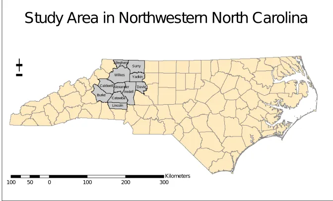
2.1.2 Study area….………14
2.1.3 Objectives.………...17
2.2 Materials and methods..………..17
2.2.1 Data…….……….18
2.2.3 Preprocessing.………..19
2.2.4 Classification method….………..19
2.2.4.1 2000 image………….………...…21
2.2.4.2 1984 image……….………...22
2.2.5 Post processing.………22
2.2.6 Accuracy assessment.………..22
2.3 Results..………...23
2.3.1 Land cover………….………..23
2.3.2 Accuracy assessment.………..24
2.4 Discussion..……….26
2.5 Conclusion..………29
Chapter 3. The effects of change in policy and practices on clear-cut harvesting in western North Carolina………..31
3.1 Introduction..………...32
3.1.1 Policies affecting forest harvesting.……….32
3.1.2 Changes in forest harvesting practices.………34
3.1.3 Objective.……….35
3.1.4 Study area….………35
3.2 Materials and methods..………..36
3.2.1 Land cover maps……….……….36
3.2.2 Landscape metric calculations……….……37
3.2.2.3 Measures of patch shape……….………..39
3.2.2.4 Measurement of association between clear-cut and physiographic region……….40
3.3 Results…..………...40
3.3.1 Overall land cover……….………...40
3.3.2 Landscape metrics………….………...42
3.4 Discussion..……….45
3.5 Conclusions..………...47
References………49
Appendix A. Leaf-on false-color composite image of study area: March 06, 2000….53 Appendix A. Final classified 2000 image after running 3x3 focal mean filter..……...54
List of Tables
Chapter 2
Table 2.1 Image data used for classification and accuracy assessment………....…18 Table 2.2 Classification scheme after modifying Anderson scheme to add a clear-cut
class and remove classes not represented in the study area.……….…19 Table 2.3 Land-cover change as a percent during the study time period..…..……….24 Table 2.4 Error matrix; producer’s and user’s accuracies for the 2000 land cover
classification……….25 Table 2.5 Error matrix; producer’s and user’s accuracies for the 2000 land cover
classification……….25 Table 2.6 Table showing kappa statistics indicating classification performance relative
to a random classification……….………26
Chapter 3
Table 3.1 Classification scheme after modifying the Anderson level 1 scheme to add a clear-cut class and remove classes not represented in the study area……37 Table 3.2 Land use and land cover change in the western piedmont of North Carolina
List of Figures
Chapter 2
Figure 2.1 11-county study area in North Carolina…..………16 Figure 2.2 Percentage of each land-cover class in the western piedmont at both time
steps………..………23
Chapter 3
Figure 3.1 11-county study area in North Carolina…..………36 Figure 3.2 Percentage cover of each land-cover class in the western piedmont at both
Chapter 1
Literature review: Changing forestry policies and practices in
North Carolina, vegetation classification, and clear-cut
1.1 Changes in harvesting policies and practices in North Carolina
1.1.1 Policy change
1.1.2 Change in practices
Forest harvesting practices in the southeastern United States have also changed during the last 25 years. In the Pacific Northwest, the timber producing heartland of America, controversy over the effects of timber harvesting on water quality and endangered or threatened species prompted forest industry to seek more hospitable political and social climates. Forest harvesting rates in North Carolina increased as the focus of forest industry shifted to the southeast. As of 1997, more wood was being harvested from the southeast than from any other wood-producing region in the world (Cubbage and Richter 1998). In addition, large areas of forest land in North Carolina have been converted to other uses between 1982 and 1997, averaging 31,000 hectares (77,000 acres) per year (Schaberg et al 2000 [2]).
To generate data for analyzing the impacts of clear-cut harvesting, clear-cuts and land cover can be located using remotely sensed satellite images. The generation of a land cover map requires the knowledge of the science of vegetation classification.
1.2 Vegetation mapping and classification
1.2.1 Basis of classification and impact of technology
Vegetation mapping in the United States began in earnest in the 19th century, and developed alongside the field of plant community ecology throughout the 20th century. Developments and theories presented in the field of plant community classification spurred new maps, and the latest maps fueled revolutions in vegetation classification theory (Kuchler 1967). Because humans can significantly alter the environment and change both what land is used for as well as what covers the ground, land use and land cover classifications have become equally as important as vegetation classifications. New technologies for data capture and analyses have been responsible in large part for the rapid advance of classification and mapping techniques in the latter part of the 20th century (Koch 2001). These advances include computers, aerial photography, and
classification should satisfy the needs of its users “with minimum cost, time, and commitment of resources” (Kimmins 1997).
1.2.2 Classification schemes
The variety of land use, land cover, and vegetation classification schemes and the approaches used to develop them are an indicator of the many applications of land use and land cover maps. It is unlikely that a single method will ever emerge, because different user needs and environmental conditions favor different approaches (Kimmins 1997). This is not intended to be a definitive list of all classification approaches; indeed, entire books are devoted to the subject. Instead, several popular approaches and their applications are described.
The Danish ecologists Warming and Raunkiar dealt only with vegetative classes (Kimmins 1997), which they defined as plant communities with similar growth forms growing in the same type of environment. In this system, called physiognomic classification, the most general classes are called formations, and associations within these formations consist of plant communities with specific compositions. This approach has proved very useful for describing vegetation on a broad scale and for comparing vegetation types between continents (Kimmins 1997).
approach (FGDC 1997). This classification system uses seven hierarchical levels, with the most general levels based on physiognomic traits and the most specific on floristic characteristics (FGDC 1997). This system allows flexibility for classifying at a very high level of detail while providing a basis for comparison of classifications between
ecosystems. While this system is the newest classification system available, it is only designed to classify vegetation, and is not a land use or land cover classification scheme.
Land use classification places areas into classes based on the anthropogenic use of an area. This can be difficult to determine without some ancillary data. Example of land use categories would be residential land, agricultural land, or pasture land. Land cover classification, on the other hand, takes into account the type of feature present on the surface of the earth. Examples of land cover classes are forested land, developed land, and grassland. Combining the two types is necessary for any task where land use must be inferred from land cover, such as when detecting clear-cuts. The US Geological Survey classification scheme, described below, is a combination of the two types of
classification.
1.3 Clear-cut detection
1.3.1 Beginnings of clear-cut detection
Clear-cut detection using remotely sensed data has traditionally focused on the tropics, particularly in the Amazon basin, where widespread clearing has resulted in the loss of 15,000 to 50,000 hectares annually beginning in 1970 (Brondizio et al. 1996). Several studies have successfully identified clear-cut areas in the Amazon using a variety of remotely sensed data sources with varying pixel sizes and image repeat intervals (Brondizio et al. 1996, Booth 1989, Skole and Tucker 1993). Early stud ies used the Advanced Very High Resolution Radiometer (AVHRR), which is designed to collect regional information on vegetation condition and water temperature daily with complete global coverage (Jensen 1996). AVHRR data has a very large pixel size (1 km per side), making it appropriate for applications involving very large areas. The Landsat
Multispectral Scanner (MSS), Landsat Thematic Mapper (TM), and Systeme Pour l'observation de la Terre (SPOT) sensors have longer repeat intervals, are designed for larger-scale applications, and have multispectral pixel sizes of 60, 30, and 20 meters per side, respectively. Many early studies involved tracing deforested area boundaries on color transparencies of satellite images rather than using spectral information to separate land cover classes. Using transparencies lowers the cost of image acquisition but has the effect of lowering resolution and spatial accuracy.
1.3.2 Clear-cut studies in the United States
detection using spectral information from Landsat TM and SPOT satellite sensors has been performed in the U.S. at an accuracy level at or above federal accuracy standards (Verbyla and Richardson, 1996), but dedicated detection efforts have been rare. Also, successful studies have been located in heavily forested areas rather than areas
undergoing extensive anthropogenic disturbance.
Government agencies state that monitoring forests is not included in their mandates, or that funds are not available for such projects (Booth, 1989). To overcome funding shortages, the Multi- Resolution Land Characteristics Consortium (MRLC) was created by several federal agencies that have committed to funding the National Land Cover Dataset (NLCD), a consistent land use and land cover dataset for the U.S. (USGS 1999). This dataset is complete and was classified using a modified Anderson (1976)
classification scheme, but clear-cuts are not separated from other transitional land cover types. The U.S. Department of Agriculture (USDA) Forest Service compiles statistics on the state of forests within US borders, but uses plot-based sampling methods rather than remotely sensed data, and does not release plot locations, citing privacy concerns.
natural disturbances mimicked by clear-cuts, finding significant differences. Clear-cutting produces a more heterogeneous landscape with smaller patches than does severe fire disturbance (Schroeder and Perera 2002).
Harvesting has been shown to change wildlife species composition. Because of their very nature, clear-cuts in a forested landscape create edge habitat and reduce forest interior habitat. Foundational research in landscape ecology states that when harvesting begins on an undisturbed forest, biodiversity increases as pioneer species populate the newly disturbed cutover area (Franklin and Foreman 1987). As harvesting continues to reduce the amount of undisturbed forest, species losses occur as the forest becomes more fragmented, culminating when all undisturbed forest is gone. This is true particularly for large interior forest dwelling carnivores such as wolves and bear. Other wildlife show opposite effects, for example, a study by Rudnicky and Hunter (1993) found that bird species diversity responds positively to increasing clear-cut size.
1.3.3 A clear-cut map for western North Carolina
The combination of changes in policy and practice in addition to shifting public
perception of natural resource management activities has prompted interest in clear-cut harvesting activities among policy makers, concerned citizen groups, and scientists. This concern is especially visible in the western North Carolina piedmont and mountains, where tourism is a valuable industry and forest products are important to local
Chapter 2
2.1 Introduction
2.1.1 Clear-cut harvesting
Clear-cut harvesting is a common forest harvesting technique in the eastern United States that involves harvesting all the trees in a forested area. While a clear-cut can be of any size, clear-cuts in the southeastern United States generally range from 4 to 60 hectares (10-150 acres) in size. Recently, in agreement with the Sustainable Forestry Initiative (SFI) and other forest certification standards, many forest products companies have voluntarily lowered their average clear-cut size to 48 hectares (SFI 2002) and set maximum individual clear-cut size limits between 60 and 90 hectares (Boston and
Bettinger 2001). These guidelines give forest mana gers some flexibility, but are designed to discourage very large clear-cut patches.
and yellow poplar (Liriodendron tulipifera), which can result in forest composition change if the regenerated forest replaces a hardwood-dominated forest type. While high levels of biodiversity are often apparent for the first years after a clear-cut, the needs of species dependent on mature forest are not provided for in stands of early successional species managed for timber (Moore and Allen 1999).
Because current legislation in North Carolina does not require landowners to report forest harvest activities, sizes, or locations, alternative methods for quantifying this landscape change must be pursued. Remote sensing using satellite data is an ideal way to approach this problem, providing multi-temporal data high in information content over a large area. High rates of growth are typical of early successional species during their first years of life, and the vigor of this growth is easily detectable by Landsat Thematic Mapper (TM) and Enhanced Thematic Mapper (ETM+) data (Jensen 1996). The characteristic remnant vegetation left after harvesting operations cause clear-cut patches to appear very
characteristically in remote sensing data (Lillesand and Kiefer, 2000), and provides a means for separating clear-cut areas from other bare earth areas using remote sensing classification techniques.
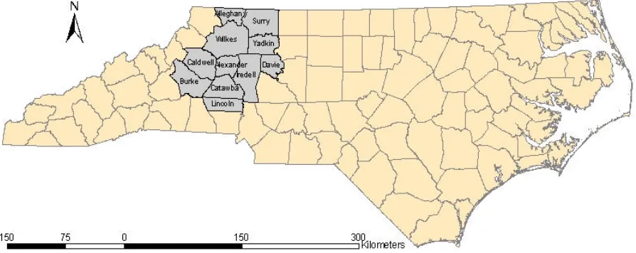
2.1.2 Study Area
Wilkes Surry
Iredell Burke
Caldwell
Yadkin
Catawba
Davie
Lincoln Alexander
Alleghany
100 50 0 100 200 300
Kilometers
±
Study Area in Northwestern North Carolina
2.1.3 Objectives
• Develop a technique to identify and map forest clear-cuts in the western piedmont
region of North Carolina using Landsat data.
• Generate land cover maps for the years 1984 and 2000 using the technique.
• Perform an assessment of classification accuracy.
2.2 Materials and Methods
All image manipulation, classification, and accuracy assessment were performed at the NC State University Center for Earth Observation (CEO) using the IMAGINE software package from Leica Geosystems (formerly ERDAS, inc.).
2.2.1 Data
accuracy assessment. Chip mill locations were available in digital format from the USDA Forest Service Southern Research Station at
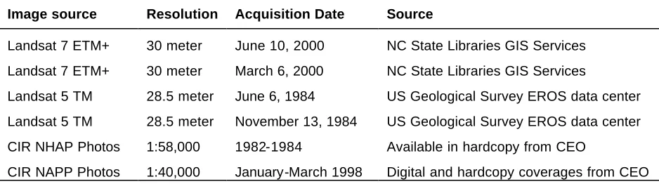
http://www.rtp.srs.fs.fed.us/econ/data/mills/chip2000.htm (Prestemon 2000). The study area occupies the western half of one Landsat scene (Path 17, Row 35). Image data information is described in Table 2.1.
Table 2.1
Image data used for classification and accuracy assessment.
Image source Resolution Acquisition Date Source
Landsat 7 ETM+ 30 meter June 10, 2000 NC State Libraries GIS Services Landsat 7 ETM+ 30 meter March 6, 2000 NC State Libraries GIS Services
Landsat 5 TM 28.5 meter June 6, 1984 US Geological Survey EROS data center Landsat 5 TM 28.5 meter November 13, 1984 US Geological Survey EROS data center CIR NHAP Photos 1:58,000 1982-1984 Available in hardcopy from CEO
CIR NAPP Photos 1:40,000 January-March 1998 Digital and hardcopy coverages from CEO
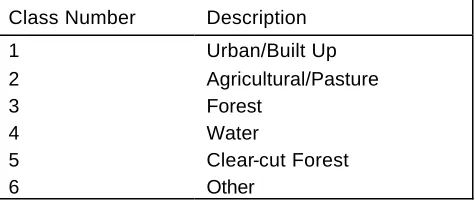
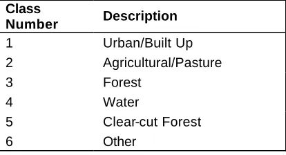
2.2.2 Classification Scheme
Table 2.2
Classification scheme after modifying Anderson scheme to add a clear-cut class and remove classes not represented in the study area.
Class Number Description 1 Urban/Built Up 2 Agricultural/Pasture 3 Forest
4 Water
5 Clear-cut Forest 6 Other
2.2.3 Preprocessing
Before classification, all Landsat images were geographically referenced to the June 10, 2000 image using 2nd order polynomial image-to-image rectification. Following
registration, boundaries of all Landsat scenes standardized using the county boundaries of the study area. Feature space images and a variance-covariance matrix were analyzed to determine which spectral bands contained the most information and to remove bands containing redundant information, reducing computation time (Jensen 1996). To separate agriculture, forest, and water, spectral subsets of bands 3, 4, and 5 were determined to contain the most information and a subset was created from each image. Using the same process, spectral subsets of each image containing bands 2, 3, and 4 were determined to contain more useful information for separating agriculture and clear-cut areas.
2.2.4 Classification
2.2.4.1 2000 Dataset
to specify the number of classes generated (Jensen 1996). The algorithm starts by determining an arbitrary number of means and assigning pixels to clusters based on the spectral distance from each mean. After assigning all of the pixels in an image, means are recalculated and pixels reassigned to the closest cluster. The process repeats
iteratively until a convergence threshold is reached representing the percentage of pixels that go unchanged between iterations. A maximum number of iterations is set because the algorithm can loop infinitely in some cases (ERDAS 2000, Ball and Hall 1965).
Temporal variation in phenology was used to help classify the remaining mixed areas for which the category was indeterminate. The spectral bands for the summer and winter images were combined into one 14-band dataset. A principal components analysis (PCA) transformation was then applied to the combined dataset. Principal components analysis is a technique used to reduce large datasets into simpler ones by capturing major axes of variation across multiple spectral bands (Lillesand and Kiefer 2000). The first five principal components explained 94.5 % of the variation in the 14-band image and were used in subsequent analyses. The PCA transformation captured seasonal variation between the two image dates in 2000. An unsupervised classification was run on the PCA image producing 25 clusters. After assigning land cover classes to each cluster, 1.43% of the image remained in mixed clusters. A final unsupervised classification produced 10 clusters, all of which could be sorted into identifiable classes.
2.2.4.2 1984 Images
To simplify classification of the 1984 image, a binary change mask was generated to identify areas that changed spectrally between 1984 and 2000. A PCA transformation was used to create the change mask by stacking the images from 1984 and 2000,
transforming the data, and using an unsupervised classification on the first few principal components. Values of change or no change were assigned to the results of the
2.2.5 Post processing
After classification, the land cover class maps for both dates were then filtered using a neighborhood focal majority analysis with a 3x3 window. The procedure simulates using a minimum mapping unit of approximately 0.8 hectare (two acres) by smoothing the “salt and pepper” effect created when isolated pixels have different classifications than those of surrounding pixels.
2.2.6 Accuracy Assessment
Accuracy assessment was performed on all categories for both the 1984 and 2000 land cover maps. 1998 Digital Orthophoto Quarter Quadrangles (DOQQs), winter and summer Landsat images, and 1999 National Aerial Photography Program (NAPP) photographs at 1:40,000 scale were the reference dataset for the 2000 classification. 1982-83 National High Altitude Photography (NHAP) program hardcopy photographs at a 1:58,000 scale, and winter and summer Landsat images were the reference dataset for the 1984 classification. Using a stratified sample, 50 points were placed randomly on the image in each land cover class for a total of 300 points in accordance with the
2.3 Results
2.3.1 Land Cover
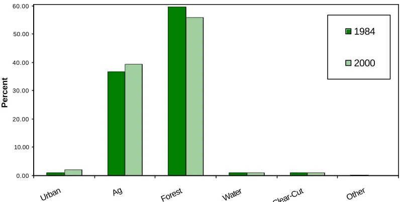
Landcover was classified according to the modified USGS Anderson classification scheme and accuracy was assessed using standard accuracy assessment techniques. Both classifications indicate that forest, followed by agriculture, are the dominant land
conditions in the northwestern Piedmont (Figure 2.2). While all land covers maintained the same relative rank between 1984 and 2000, significant changes in land cover did occur within each category.
0.00 10.00 20.00 30.00 40.00 50.00 60.00
Urban Ag Forest Water
Clear-Cut Other
Percent
1984 2000
Figure 2.2. Percentage cover of each land-cover class in the western Piedmont at both time steps.
decrease (-42,916 ha) in forested area. Water increased about 10% in area between time steps due to slightly higher water levels in 2000 vs. 1984 and the construction of several reservoirs between 1984 and 2000.
Table 2.3
Land-cover change as a percent during the study time period.
Cover type 1984 area km2 (mi2) 2000 area km2 (mi2) Percent change
Urban 145.30 (56.10) 269.38 (104.07) 84.8% Ag 4471.87 (1726.60) 4808.67 (1856.64) 7.1% Forest 7253.70 (2800.67) 6824.54 (2634.97) -6.3% Water 125.61 (48.50) 137.99 (53.28) 9.4% Clear-Cut 121.44 (46.89) 130.10 (50.23) 6.7% Other 17.22 (6.65) 10.49 (4.05) -39.2% Total 12135.16 (4685.41) 12181.36 (4703.25)
Comparison of the 2000 and 1984 land cover maps reveals that 63.7% of the clear-cut area identified in 1984 returned to forest cover, while 26.5% of clear-cut area became agriculture. Nine percent of 1984 clear-cut area was still recognizable as clear-cut using the 2000 classification because of misclassified agricultural areas, slow re-growth of some harvested areas, and clearing for development misidentified as clear-cut area. 2.3.2 Accuracy Assessment
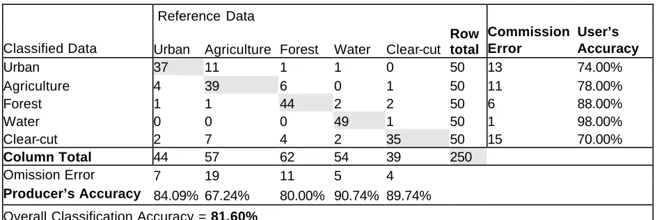
The final error matrices as well as user’s and producer’s accuracies are listed in tables 2.4 and 2.5. Producer’s accuracy indicates the probability of a reference pixel being
correctly classified, and user’s accuracy indicates the probability that a pixel’s
is identified on the ground, there is a high probability that the clear-cut will be identified on the map as such, at the expense of including some land as “false positives”.
Table 2.4
Error matrix; producer's and user's accuracies for the 2000 land cover classification.
Reference Data
Classified Data Urban Agriculture Forest Water Clear-cut
Row total Commission Error User’s Accuracy
Urban 37 11 1 1 0 50 13 74.00% Agriculture 4 39 6 0 1 50 11 78.00% Forest 1 1 44 2 2 50 6 88.00% Water 0 0 0 49 1 50 1 98.00% Clear-cut 2 7 4 2 35 50 15 70.00%
Column Total 44 57 62 54 39 250
Omission Error 7 19 11 5 4
Producer’s Accuracy 84.09% 67.24% 80.00% 90.74% 89.74%
Overall Classification Accuracy = 81.60%
Table 2.5
Error matrix; producer's and user's accuracies for the 1984 land cover classification.
Reference Data
Classified Data Urban Agriculture Forest Water Clear-cut
Row total Commission Error User’s Accuracy
Urban 32 3 3 1 0 39 7 82.05% Agriculture 4 21 2 0 3 30 9 70.00% Forest 0 4 24 0 1 29 5 82.76% Water 0 0 0 24 0 24 0 100.00% Clear-cut 0 10 2 3 12 27 15 44.44%
Column Total 36 38 31 28 16 149
Omission Error 4 17 7 4 4
Producer’s Accuracy 88.89% 55.26% 77.42% 85.71% 75.00%
Overall Classification Accuracy = 75.84%
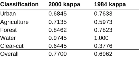
that all cover types are reliably identified in both classifications. All condition classes were shown to be far better than a random classification in cover type maps from both years. Overall kappa is 0.7700 for the 2000 classification and 0.6962 for the 1984 classification. The kappa corresponding to the clear-cut class is significantly lower for the 1984 classification than for the 2000 classification, but can be thought of as 69% better than a random classification (Lillesand and Kiefer, 2000). The low kappa value for the clear-cut class is due to the low user’s accuracy component, signifying an
over-predication of clear-cuts. Table 2.6.
Table showing kappa statistics indicating classification performance relative to a random classification.
Classification 2000 kappa 1984 kappa
Urban 0.6845 0.7633 Agriculture 0.7135 0.5973 Forest 0.8462 0.7823 Water 0.9745 1.000 Clear-cut 0.6445 0.3776 Overall 0.7700 0.6962
2.4 Discussion
Unsupervised classification also made the task of classifying an area without a priori knowledge easier. As the ISODATA routine separated spectrally different areas into clusters, any troublesome or unknown areas could be identified with aerial photography on an as needed basis rather than before the classification, as would ha ve been necessary with a supervised classification technique. This removed the need for a detailed
knowledge of the study area before the study began and made it possible to handle errors in classification as they occurred rather than attempting to anticipate errors.
Due in part to variations in topography, elevation, plant community age structure, and moisture regimes present throughout the study area, there were many spectral
representations for each cover type. Occasionally these factors cause non-clear-cut areas to appear similar to the spectral representation of clear-cut areas. Agriculture was
mistaken most often for clear-cut, with forest a distant second. Because the percentage of the study area classified as clear-cut is small, the amount of fo rest and agriculture
misclassified as clear-cut is probably a very small percentage of the total area for those cover types. The high producer’s accuracy and especially low user’s accuracy indicates that clear-cut area may be substantially overestimated in the 1984 classification. If true, the increase in clear-cut area for the 16- year study period may have been even larger than the 6.7% found here.
variation in landforms throughout the image area. The coarse image quality was an issue during image registration, because pixels in a coarse-resolution image are often made up of reflectance from multiple sources. The boundaries between these sources are rarely coincident with the boundaries between pixels; hence matching points between remotely sensed images can be exceedingly difficult (Jensen 1996). Similarities between class appearances were more pronounced on the 1984 image, where classification involved considerably more effort due to poorer 1984 image quality and available imagery dates. Compared to the 2000 Landsat 7 ETM+ image, the 1984 Landsat 5 TM dataset had lower contrast, tended to be grainier, and had an abundance of clouds obscuring the image clustered along the western edge of the study area. Specifically, compacted/developed surfaces and agriculture were difficult to distinguish, and low, scrubby, forest vegetation appeared similar to some herbaceous pasture areas. Accuracy was degraded due to this fact, resulting in more overestimation of clear-cut area in 1984 than in 2000. Image collection date also had adverse effects on accuracy. Winter Landsat ETM+ imagery for 2000 was collected in March, providing clear distinction between forest and agricultural areas. Use of November imagery in 1984 concealed some of this distinction and was reflected in the lower classification accuracy for the 1984 dataset. This made discerning clear-cut areas on the 1984 images a much more difficult task than using the 2000 images.
interpretable image (Lillesand and Kiefer 2000) and leading to better clear-cut detection accuracy. Using a low-pass filter and a contrast stretch may have mitigated for some of the image quality problems in the 1984 image. Because the study area included
mountainous terrain, normalizations for slope and shadow could have led to further improvements in classification accuracy for both dates. These techniques were not employed due to the exploratory nature of the study, but could prove useful in future mapping efforts. Other possible improvements include using a smaller study area to reduce variation in cover types, limiting the study area to a more homogenous, forested area, or examining an area with less variation in elevation.
2.5 Conclusions
The goals of this study were to devise a method of clear-cut detection, use the method to generate a land cover map for the western piedmont of North Carolina, and to assess the accuracy of that classification. This study determined that detection of clear-cut areas is feasible using Landsat TM and ETM+ data and standard remote sensing techniques. Unsupervised classification was crucial in allowing classification to take place without a priori knowledge of the study area. The deliberate overestimation of clear-cut area to ensure capture of all clear-cut areas in the correct class was another advantage of the classification technique used in this study. While there are certainly improvements that would almost certainly improve the accuracy of this process, it is worth noting that overall classification accuracy exceeds the USGS/National Park Service standards of 80% accuracy in thematic classifications for 2000, and is very close for 1984.
Chapter 3
The effects of change in policy and practices on clear-cut
3.1 Introduction
3.1.1 Policies affecting forest harvesting
Over the last 40 years, the attitude of the American public regarding natural resources has changed (Kessler et al. 1992). This has led to a variety of policy changes directed at changing the way forests are used for profit and to benefit the public good.
size, shape, and configuration, and species mobility, population size, and reproductive capacity.
Voluntary limits to clear-cut size are another policy change that has occurred due to shifting perceptions and attitudes about natural resources. The Sustainable Forestry Initiative (SFI) program, endorsed by the American Forest and Paper foundation, is a program that enforces a maximum average clear-cut size of 48 hectares (120 acres) in any year for all the land a company manages (Sustainable Forestry Initiative 2002). This guideline allows forest managers the flexibility to use large clear-cut harvests when necessary, but discourages the practice of using many very large clear-cuts. Forest products companies must adhere to these standards to maintain membership in the
3.1.2 Changes in forest harvesting practices
Forest harvesting practices in the Southeast have also changed during the last 25 years. In the Pacific Northwest, the timber producing heartland of America, controversy about the effects of timber harvesting on water quality and endangered or threatened species prompted forest industry to seek more a hospitable and profitable political climate. Forest harvesting rates increased in North Carolina as the focus of forest industry shifted from the Pacifica Northwest to the Southeast. By 1997, more wood was being harvested from the Southeast than from any other wood-producing region in the world (Cubbage and Richter, 1998). In addition, large areas of forest have been converted to other uses in North Carolina between 1982 and 1997, averaging 31,000 hectares (77,000 acres) per year (Schaberg et al 2000 [2]).
The introduction of chip mill harvesting technology has also raised concerns, particularly in western North Carolina. Chip mills are designed to efficiently use the wood of smaller diameter trees than traditional sawmills, thus opening more areas to harvest and
3.1.3 Objective
The overall goal of this stud y was to quantify the effects of changes in the policies and practices affecting clear-cut forest harvesting on clear-cut harvesting patterns. The effects of these changes were examined using land cover maps for 1984 and 2000 generated by Bailey (in preparation). Each hypothesis is related to a specific change in landscape composition that could be caused by a change in forest policy or practice between 1984 and 2000.
Four hypotheses were tested:
• H1: The distribution of clear-cut patch sizes changed significantly between 1984
and 2000.
• H2: Average shortest distance between clear-cut patches and chip mills changed
significantly during the study time period.
• H3: Harvest levels have increased in mountainous areas.
• H4: Forest patch shape has become more linear over the study time period.
3.1.4 Study area
agriculture (39% in 1990) (Bailey in preparation). A wide range of forest types include loblolly pine plantations, oak-hickory uplands, nearly pure stands of yellow poplar and white pine, and high-elevation spruce- fir. Throughout the study area, particularly towards the east, the landscape consists of a mosaic of forest and agriculture, with very
fragmented forested areas. Counties were selected for study based on the large
percentage of forest cover and the presence of chip mills within the area. According to geographic data compiled in 2000, 13 mills are located inside or within 50 miles of this study area, 10 of which began operation after 1984 (Prestemon et al. 2000). 50 miles is the typical range from within which a chip mill will receive trees.
Figure 3.1 11-county study area in North Carolina.
3.2 Materials and methods
3.2.1 Land cover maps
accurately using remotely sensed satellite data. Both maps covered the same study area, with a land area slightly less than 13,000 square kilometers (5,019 mi2). These land cover data were used for all hypotheses tests. Land cover was classified using a USGS Anderson level 1 land cover classification scheme modified to remove categories not present in North Carolina and add clear-cut and other categories as described in table 3.1 (Anderson et al. 1976).
Table 3.1
Classification scheme after modifying the Anderson level 1 scheme to add a clear-cut class and remove classes not represented in the study area.
Class
Number Description
1 Urban/Built Up 2 Agricultural/Pasture 3 Forest
4 Water
5 Clear-cut Forest 6 Other
Overall accuracy was 82% for the 2000 land cover map and 76% for the 1984 land cover map. Because the clear-cut detection study was concerned with capturing all clear-cut areas in the correct class, non-clear-cut areas were occasionally wrongly assigned to the clear-cut class.
3.2.2 Landscape metric calculations
3.2.2.1 Measures of patch size
that increasing patch size has a significant positive effect on classification accuracy, so that small patches tend to be classified incorrectly. For this reason, analyses of clear-cut patches and forest patches were restricted to patches greater than 5 pixels in size,
approximately 4,500 m2 (one acre). Economic factors generally prohibit clear-cutting on areas smaller than 1 acre, so it is likely that very small patches are non-clear-cut areas with spectral signatures similar to clear-cut patches.
Summary statistics calculated include the total number of patches, mean patch size, and quantiles for each distribution, as well as histograms. Because of the large number and broad range of clear-cut patch sizes, comparing means between datasets can be
misleading. More thorough analysis of large samples can be conducted by comparing distributions of patch size. The Kolmogorov-Smirnov (K-S) two-sample test for a common distribution was used to compare distributions of several variables from each year. The Kolmogorov-Smirnov test is a non-parametric test designed for continuous data, with assumptions that hold for data distributed non-normally. The null hypothesis for this test states that both sets of observations come from identical distributions. A rejection of the null hypothesis can reflect change in location, skewness, or variance (Sprent and Smeeton 2001).
3.2.2.2 Measurement of distance between clear-cuts and chip mills
mill. The Kolmogorov-Smirnov test, histograms, and summary statistics were used to compare distance distributions for each year.
3.2.2.3 Measures of patch shape
Forest patch linearity was estimated by measuring patch elongation and patch complexity using the shape index and related circumscribing circle metrics. The shape index metric is a measure of shape complexity calculated by comparing patch perimeter and the minimum patch perimeter possible for a square patch of the same area. (McGarigal et al. 2002). Because shape index uses a square or almost square area for comparison, it corrects for the size sensitivity present when using a simple perimeter-area ratio. Shape index is equal to 1 when a patch is maximally compact, and increases without limit as patch shape becomes more irregular.
The related circumscribing circle metric is a measure of patch elongation based on the minimum area of a circle that could surround the entire patch. Related circumscribing circle is equal to zero for circular patches and approaches one for elongated, narrow patches one cell wide (McGarigal 2002).
3.2.2.4 Measurement of association between clear-cut and physiographic region
To examine changes in clear-cutting practices in the mountain physiographic region, elevation value s were assigned to each pixel classified as clear-cut for both time periods using a 30- meter Digital Elevation Model (DEM) covering the study area (McCoy 2001). Calculating the area of all cells classified as clear-cut with elevation values higher than 610 meters (2000 feet) provides a good estimate of the amount of clear-cut area within the study area in the mountain physiographic region rather than the piedmont.
3.3 Results
3.3.1 Overall land cover
Forest and agriculture were the dominant land cover in the northwestern Piedmont in both 1984 and 2000 (Figure 3.2). While all land covers maintained the same relative rank between 1984 and 2000, changes in land cover occurred within each category (Table 3.2). Most notably, urban land cover increased in area by 84.8% of the urban value in 1984 (4,123 ha). Forest land showed a 6.7% decrease from the amount of forest area in 1984, representing 42,900 hectares.
The increase in urban area came at the expense of forest and agricultural area (Table 3.2). Agriculture gained area from the conversion of forest resulting in a 6% decrease in
0.00 10.00 20.00 30.00 40.00 50.00 60.00
Urban Ag Forest Water
Clear-Cut Other
Percent
1984 2000
Figure 3.2 Percentage cover of each land-cover class in the western Piedmont at both time steps.
Clear-cut area increased 7%. Underestimation of clear-cut land area in the 1984 classification may mean that the true increase in clear-cut area may be larger than 7%. Misclassifications in the datasets used in this analysis account for the unlikely estimates of change from urban to other classes. Confusion between forest and urban classes can be common in remotely sensed datasets.
Table 3.2
Land use and land cover change in the western piedmont of North Carolina between 1984 and 2000. Highlighted categories indicate land that did not change classes during the study perio d. Read across the table to find the number of hectares converted from a category into a new use between 1984 and 2000. Read down the table to find the sources hectares converted into a new use between 1984 and 2000. (Table format and terminology adapted from Hess et al. 1999)
|---1984-2000 Land Use Change (Hectares)---|
1984 Land Use (Hectares) Urban Agriculture Forest Water Clear-cut Other
Urban 16,099 13,445 2,075 540 10 7 20
Agriculture 490,311 10,948 406,634 68,580 99 3,890 159
Forest 788,701 4,930 112,000 661,677 859 8,995 241
Water 13,897 23 79 701 13,092 0 2
Clear-cut 13,440 97 3,505 8,564 1 1,272 0
Other 868 7 92 718 7 10 34
2000 Land Use (hectares) 29,450 524,385 740,781 14,068 14,174 457
Looking specifically at clear-cut regeneration, it was found that 64% of the clear-cut area identified in 1984 returned to forest cover, while 26% of clear-cut area became
agriculture. Nine percent of clear-cut area was still recognizable as clear-cut using the 2000 classification, either because the areas had been cut again, or because vegetation regrowth over 16 years was insufficient to cause the areas to appear as forests in the classification. Less one percent of identified clear-cuts in 1984 became urban.
3.3.2 Landscape metrics
Using the Kolmogorov-Smirnov test to compare the distributions of clear-cut patch sizes yielded a p- value of < .0001, indicating that the distribution of clear-cut sizes changed significantly between 1984 and 2000. Most notably, the number of clear-cut patches increased from 5,377 to 6,081 (13.1%), while the mean clear-cut patch size decreased from 1.63 ha to 1.45 ha (12.4%). The distribution of patch sizes was heavily skewed towards smaller patch sizes in both datasets, with only a few very large patches present.
3367 1126 375 305 89 3610 1497 474 363 79 0 500 1000 1500 2000 2500 3000 3500 4000
0-1 1-2 2-3 3-6 6-9
Patch Size Category (Hectares)
Patch Frequency
1984 2000
Figure 3.3 Frequency distribution of clear-cut patch sizes smaller than 9 hectares. The 2000 dataset has noticeably more small clear-cut patches compared to the 1984 dataset.
86 26 2 0 1 51 6
0 1 0
0 10 20 30 40 50 60 70 80 90 100
9-20 20-55 55-90 90-125 125-160
Patch Size Category (Hectares)
Patch Frequency
1984 2000
Comparison of the means for shape index and nearest circumscribing circle metrics showed little change between 1984 and 2000. Forest patches displa yed a tendency to be slightly elongated (CIRCLE = .58 for both years) but not particularly irregular (SHAPE = 1.59 for 1984 and SHAPE = 1.60 for 2000) on both dates. Standard deviations were similar for both metrics between years.
Average distance from clear-cut patch to the closest chip mill increased between 1984 and 2000, from 38.6 km (24.0 mi) to 43.0 km (26.7 mi). Using the Kolmogorov-Smirnov test, we were able to reject the null hypothesis that the distribution of clear-cut patch to mill distances was identical for both years with a p-value <.0001. While the distribution shapes are similar and are somewhat bimodal in appearance, the 2000 dataset is skewed towards larger distances compared to the 1984 dataset (figure 3.5).
0 50 100 150 200 250 300 350 400 450
0 6 12 18 24 30 36 42 48 54 60 66 72 78 84 90
Distance to closest chip mill from clear-cut patch (km)
Frequency
1984
2000
Examination of clear-cut patches with respect to elevation reveals that the amount of clear-cut area present in mountainous areas (those areas at and above 610 meters [2000 ft] in elevation) increased from 456 hectares to 1169 hectares, an increase of over 150% between time periods.
3.4 Discussion
The measurable decline in clear-cut patch size and increase in the number of clear-cut patches are indications that forest harvesting practices are being altered in the manner suggested by SFI and other voluntary standards. The number of large clear-cut patches decreased, while the overall amount of land harvested increased. An increase in small patches accounts for the majority of increased ha rvesting levels.
Increasing the number of small clear-cut patches while maintaining or increasing the area harvested may lead to habitat fragmentation for some species by shrinking and breaking apart contiguous forest habitat areas. Because green-up constraints prohibit the harvest of adjacent patches generally within 3 years of one another, a clear-cut can be the source of forest fragmentation even when cuts are not dispersed over the landscape. When adjacent patches of the same forest type are regene rated at different times the resulting stands may differ in structure to such a degree that the stands may not provide a contiguous habitat for a species.
mills have been introduced in western North Carolina. Demand in local, regional, and national markets for wood products and shifting national focus of timber production from the Pacific Northwest to the Southeast are all potential reasons for this observed increase.
The average distance from chip mill to clear-cut patch increased during the study time period, which suggests that chip mills do not attract clear-cutting to the immediate mill vicinity. Because the number of clear-cuts increased in northwestern portion of the study area, and chip mills are predominantly located in the southeastern portion of the study area, average distance increased. Measuring average distance may not have been a definitive way to test this hypothesis. Overlapping mill sourcing areas, harvesting for traditional lumber mills, and changing transportation routes all affect clear-cut locations and distance between mill and harvest site.
Harvesting in mountainous areas over 2000 feet in elevation increased between 1984 and 2000. This can potentially lead to increased pressure on healthy animal and plant
populations that depend on the close proximity of a wide variety of habitat types present in the mountains. Improvement in access routes to the western mountains, change in tree species desired by forest products companies, and decrease in supply in the areas
There are several reasons for forest patch shape showing no discernable trend during the study time period time period. Future analysis should focus on forests near streams rather than all forests, since forests without streams are not subject to BMP regulations and should show no change. Using ancillary stream data to select forest areas near streams would help to more appropriately define the sample dataset. It is also likely that the effects of BMP regulations and 50-foot wide streamside management zones occur on such a small scale that 30- meter resolution Landsat data are too coarse to use for these measurements. In many cases buffers were less than one pixel wide and boundaries between buffer and clear-cut areas unclear. A more appropriate dataset for this type of analysis might be small-scale (1:40,000) NAPP aerial photography. Visual examination of the landcover maps used in this study along with aerial photography used for accuracy assessment by Bailey (in preparation) suggests that streamside buffers are being used more frequently in 2000 than 1984, however, metrics generated in this study did not detect these changes for the reasons listed above.
3.5 Conclusions
patches across the landscape. Franklin and Forman (1987) found that clear-cutting small, non-adjacent forest patches, rather than harvesting contiguous blocks of forest, can lead to a decline in species diversity when habitat used by interior forest dwelling species is harvested and becomes unsuitable.
The report “Economic and ecological impacts associated with wood chip production in North Carolina” by Schaberg et al. (2000 [1]) suggests that the economic impetus behind the increased harvest levels observed between 1984 and 2000 are still present. Further monitoring may help determine if increased harvesting will lead to further dispersal of clear-cut patches and fragmentation of forest throughout the landscape. It is also worth noting that forest harvesting expanded in mountainous areas during the study period. This trend may also require further monitoring to assess the cause of this change and the potential effects on montane plant and animal communities.
References
Anderson, J.R., Ernest E. Hardy, John T. Roach and Richard E. Witmer. 1976. “A Land Use and Land Cover Classification System for Use with Remote Sensor Data.”
Geological Survey Professional Paper 964. United States Government Printing Office. Washington D.C.
Bailey (in prep). 2003. Chapter 2: Clear-cut detection using remotely sensed data. NC State University Master’s Thesis. NC State University, Raleigh, NC.
Ball, G. H., and Hall, D. J. 1965. ISODATA, a novel method of data analysis and pattern classification. Technical Report, Stanford Research Institute, Melo Park, California, USA.
Barrett, T.M., J.K. Gilless, and L.S. Davis. 1998. Economic and fragmentation effects of clearcut restrictions. Forest Science 44(4): 569-577.
Brondizio, E., E. Moran, P. Mausel, and Y. Wu. 1996. Land Cover in the Amazon Estuary: Linking of the Thematic Mapper with Botanical and Historical Data. Photogrammetric Engineering and Remote Sensing 62(8): 921-929.
Booth, William. 1989. Monitoring the Fate of Forests from Space. Science 243(4897): 1428-1429.
Boston, Kevin and Pete Bettinger. 2001. The economic impact of green- up constraints in the southeastern United States. Forest Ecology and Management 145: 191-202.
Congalton, R.G. 1991. A Review of Assessing the Accuracy of Classification of Remotely Sensed Data. Remote Sensing of the Environment 37: 35-46.
Cubbage, Frederick W. and Daniel D. Richter. 1998. Economic and Ecologic Impacts Associate with Wood Chip Production in North Carolina. Cooperative Research Proposal from the Southern Center for Sustained Forests to North Carolina Department of
Environment and Natural Resources. Available from World Wide Web: <http://www.env.duke.edu/scsf/Woodchip/chip.pdf>
ERDAS, Inc. 1999. ERDAS Imagine® Field Guide, Fifth Edition. ERDAS Inc., Atlanta, GA. 282p.
Environmental Systems Research Institute (ESRI). 1994. Cell- Based Modeling with GRID. ESRI. Redlands, CA.
Federal Geographic Data Committee (FGDC). 1997. National Vegetation Classification Standard. Federal Geographic Data Committee Secretariat, c/o U.S. Geological Survey, Reston, VA. 22p.
Franklin, Jerry F. and Richard T.T. Forman. 1987. Creating landscape patterns by forest cutting: Ecological consequences and principles. Landscape Ecology 1(1): 5-18.
Hess, G.R. 1996. Disease in Metapopulation Models: Implications for Conservation. Ecology 77(5): 1617-1632.
Hess, George, Kate Dixon, and Mary Woltz.1999. State of Open Space in the Triangle. Triangle Land Conservancy [online]. Available from World Wide Web: <http://www.tlc-nc.org/sos2000.pdf>
Jensen, J.R., 1996. Introductory Digital Image Processing. Prentice Hall, Inc. New Jersey. Kessler, Winifred B., Hal Salwasser, Charles W. Cartwright Jr., and James A. Caplan. 1992. New Perspectives for Sustainable Natural Resources Management. Ecological Applications 2(3): 221-225.
Kimmins, J.P. 1997. Ecosystem Classification: the Ecological Foundation for Sutainable Forest Management (Chapter 16). In Forest Ecology: A Foundation for Sustainable Management, Prentice Hall, Upper Saddle River, NJ, pp. 449-472.
Koch, Jr., Frank H. 2001. A Comparison of Digital Vegetation Mapping and Image Orthorectification Methods using Aerial Photography of Valley Forge National Historical Park. Master’s thesis, NC State University, Raleigh, NC. 126p.
Kuchler, A. W. 1967. Vegetation Mapping. The Ronald Press Company, New York. Lillesand, Thomas M., and Ralph W. Kiefer. 2000. Remote Sensing and Image Interpretation. John Wiley & Sons, Inc. New York.
Lord, Janice M. and David A. Norton. 1990. Scale and the Spatial Concept of Fragmentation. Conservation Biology 4(2): 197-202
McCoy, Jill and Kevin Johnston. 2001. Using ArcGIS Spatial Analyst. ESRI. Redlands, CA.
McGarigal, K., S. A. Cushman, M. C. Neel, and E. Ene. 2002. FRAGSTATS: Spatial Pattern Analysis Program for Categorical Maps. Computer software program produced by the authors at the University of Massachusetts, Amherst. Available from World Wide Web: <http://www.umass.edu/landeco/research/fragstats/fragstats.html>
Muller, Etienne. 1997. Mapping riparian vegetation along rivers: Old concepts and new methods. Aquatic Botany 58(1997): 411-437.
NC Division of Forest Resources. 1989. Forest Practices Guidelines Related To Water Quality. NC Department of Environment, Health, and Natural Resources, Raleigh, NC. 8p.
Rudnicky, Tamia C., and Malcolm L. Hunter Jr. 1993. Reversing the Fragmentation Perspective: Effects of Clearcut Size on Bird Species Richness in Maine. Ecological Applications, 3(2): 357-366.
Prestemon, Jeff, John Pye, David Butry, and Dan Stratton. 2000. Locations of Southern Wood Chip Mills for 2000 [online]. Available from World Wide Web: <
http://www.srs.fs.usda.gov/econ/data/mills/chip2000.htm>
Schaberg, Rex, Frederick W. Cubbage, and Daniel D. Richter. 2000 [1]. Trends in North Carolina timber product outputs, and the prevalence of wood chip mills. Paper prepared for the study on: Economic and ecological impacts associated with wood chip production in North Carolina. Available from World Wide Web:
<http://www.env.duke.edu/scsf/chip2.pdf>
Schaberg, Rex, P.B. Aruna, Frederick Cubbage, Daniel Richter, George Hess, Robert Abt, James Gregory, Sarah Warren, Anthony Snider, Brandon Greco, Stacy Sherling, and John Dodrill. 2000 [2]. Abstract of study results: Economic and ecological impacts associated with wood chip production in North Carolina. Final Report prepared by the Southern Center for Sustainable Forests [online]. Available from World Wide Web: <http://www.env.duke.edu/scsf/chipabstract.PDF>
Schroeder, David, and Ajith H. Perera. 2002. A comparison of large-scale spatial vegetation patterns following clearcuts and fires in Ontario’s boreal forests. Forest Ecology and Management 159: 217-230.
Seymour, R.S. and M.L. Hunter Jr. 1999. Principles of Ecological Forestry. In
Maintaining Biodiversity in Forest Ecosystems. Cambridge, England: Cambridge Press. Simberloff, Daniel, and James Cox. 1989. Consequences and Costs of Conservation Corridors. Conservation Biology 1(1): 63-71.
Skole, David, and Compton Tucker. 1993. Tropical Deforestation and Habitat Fragmentation in the Amazon: Sattelite Data from 1978 to 1988. Science 260(5116): 1905-1910.
Sprent, P., and N.C. Smeeton. 2001. Applied Nonparametric Statistical Methods. Boca Raton, Florida: Chapman and Hall/CRC.
Sustainable Forestry Initiative. 2004-2004 The Sustainable Forestry Initiative Standard (SFIS). 2002. Sustainable Forestry Board and the American Forest and Paper
Association [online]. Available from World Wide Web:
<http://www.sampsongroup.com/acrobat/2002-2004%2520Standard.pdf>
Thornbury, William D. 1965. Regional Geomorphology of the United States. New York, New York: John Wiley & Sons, Inc.
USGS. 1999. National Land Cover Data: Mapping Procedures. In National Land Cover Characterization [online]. Available from World Wide Web:
<http://landcover.usgs.gov/mapping_proc.asp>
Verbyla, D.L. and C.A. Richardson. 1996. Remote sensing clearcut areas within a forested watershed: Comparing SPOT HRV Panchromatic, SPOT HRV multispectral, and Landsat Thematic Mapper Data. Journal of Soil and Water Conservation 51(5): 423-427.
Appendix A. Leaf-off false-color composite image of study area: March 06, 2000.
Appendix C. Landscape metric calculations
Patch size calculation
Patch size was calculated by running a regiongroup function on the land cover data sets from both years using ArcGIS GRID (McCoy 2001). The regiongroup function assigns classified cells to patches based on proximity and calculates the size of each patch (ESRI 1994). The eight- neighbor rule, by which cells are assigned to the same patch if they share a common border or a corner, was enforced during this procedure.
The command was executed as follows:
PatchGrid = regiongroup(in_grid, #, EIGHT, WITHIN, #, #)
Shortest average distance from clear-cut to chip mill calculation
Shortest average distances from each clear-cut patch to the nearest chip mill were
Appendix C. Landscape metric calculations (Continued)
Shape Index Metric Formula (from McGarigal 2002) Formula used to calculate the shape index metric.
ij ij p p SHAPE min =
Minimum Circumscribing Circle Metric Formula (from McGarigal 2002) Formula used to calculate the related circumscribing circle metric.
− = s ij ij a a CIRCLE 1
pij = perimeter of patch ij in terms of number of cell surfaces.
min pij = minimum perimeter possible for a patch with the same
area as patch ij in terms of number of cell surfaces.
aij = area (m 2
)of patch ij. aij
s