The development of cloud modelling and motion analysis for virtual environment

(1)

THE DEVELOPMENT OF CLOUD MODELLING AND MOTION

ANALYSIS FOR VIRTUAL ENVIRONMENT

(PEMBANGUNAN PERMODELAN AWAN DAN ANALISA

PERGERAKAN UNTUK PERSEKITARAN MAYA)

MOHD SHAHRIZAL SUNAR

DAUT DAMAN

SARUDIN KARI

NORHAIDA MOHD SUAIB

ABDULLAH BADE

RESEARCH VOTE NO:

74079

JABATAN GRAFIK KOMPUTER DAN MULTIMEDIA

FAKULTI SAINS KOMPUTER DAN SISTEM MAKLUMAT

UNIVERSITI TEKNOLOGI MALAYSIA

(2)

B

O

R

A

N

G

P

E

N

G

E

S

A

H

A

N

L

A

P

O

R

A

N

A

K

H

I

R

P

E

N

Y

E

L

I

D

I

K

A

N

TAJUK PROJEK : THE DEVELOPMENT OF CLOUD MODELLING AND MOTION ANALYSIS FOR VIRTUAL ENVIRONMENT

Saya MOHD SHAHRIZAL BIN SUNAR

(HURUF BESAR)

mengaku membenarkan Laporan Akhir Penyelidikan ini disimpan di Perpustakaan Universiti Teknologi Malaysia dengan syarat-syarat kegunaan seperti berikut:

1. Laporan Akhir Penyelidikan adalah hak milik Universiti Teknologi Malaysia.

2. Perpustakaan Universiti Teknologi Malaysia dibenarkan membuat salinan untuk tujuan pengajian sahaja.

3. Perpustakaan dibenarkan membuat salinan Laporan Akhir Penyelidikan ini bagi kategori

TIDAK TERHAD. 4. *Sila tandakan ( 9 )

SULIT (Mengandungi maklumat yang berdarjah keselamatan atau kepentingan Malaysia seperti yang termaktub di dalam AKTA RAHSIA RASMI 1972)

TERHAD (Mengandungi maklumat TERHAD yang telah ditentukan oleh organisasi/badan di mana penyelidikan dijalankan)

9 TIDAK TERHAD

______________________________

(TANDATANGAN KETUA PROJEK)

Nama & Cop Ketua Penyelidik

Tarikh: 15/11/2005

(3)

ABSTRACT

(4)

ABSTRAK

(5)

TABLE OF CONTENTS

CHAPTER TITLE PAGE

DECLARATION

ABSTRACT i

ABSTRAK ii

LIST OF TABLES vi

LIST OF FIGURES vii

LIST OF ABBREVIATIONS ix

LIST OF APPENDICES x

I INTRODUCTION 1

1.1 Introduction 1

1.2 Motivation 4

1.3 Problem Background 5

1.4 Problem Statement 9

1.5 Objective of the Study 9 1.6 Importance of the Study 10

1.7 Scope of the Study 11

1.8 Thesis Contributions 11 1.9 Thesis Organization 12

II CLOUD MODELING 14

2.1 Introduction 14

2.2 Texture Mapping Techniques 15 2.2.1 Two-Dimensional Texturing 16 2.2.2 Three-Dimensional Texturing – Solid

Texturing 19

(6)

2.3.1 Polygonal and Patch Modeling 21 2.3.2 Constructive solid Geometry Models 22 2.3.3 Particle Systems 23 2.3.4 Procedural Modeling 24 2.4 Modeling Natural Phenomena 25

2.4.1 Modeling Terrain and Vegetation 25 2.4.2 Modeling Fire and Water 25 2.4.3 Modeling and Animating Gaseous

Phenomena 26

2.5 Modeling Fuzzy Objects 27 2.5.1 Particle Systems 28

2.5.2 Metaballs 29

2.5.3 Voxel Volumes 29

2.5.4 Procedural Noise 30 2.5.5 Textured Solids 31 2.6 Cloud Dynamics Simulation 32 2.7 Light Scattering and Cloud Radiometry 34

2.7.1 Spherical Harmonics Methods 35 2.7.2 Finite Element Methods 37 2.7.3 Discrete Ordinates 38 2.7.4 Monte Carlo Integration 39 2.7.5 Line Integral Methods 40 2.8 Virtual Environment 42

2.8.1 Immersion 43

2.8.2 Interaction 44

2.9 Summary 44

III PARTICLE SYSTEMS 47

3.1 Introduction 47

3.2 Use of Particles System 49

3.3 Summary 57

IV RANDOMIZED ALGORITHM

(7)

4.1 Introduction 59 4.2 Flow Diagram of Shaping Modeling Algorithm 60

4.3 Input Data 61

4.3.1 Cloud Centre 61

4.3.2 Number of Particles 61

4.3.3 Radius 61

4.3.4 Data File Format 62

4.4 Data Acquisition 64

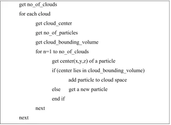
4.5 Design of Shape Modeling Algorithm 65 4.5.1 Model Formulation 66 4.5.2 Pseudo Code of Shaping

Modeling Algorithm 69 4.6 Implementation of Randomized Algorithm

in Cloud Editor 70

4.7 Summary 75

V TESTING AND RESULTS 77

5.1 Introduction 77

5.2 Efficiency of the Randomized Algorithm 78 5.3 Rendering Performance Tests 80

5.4 Summary 89

VI DISCUSSION AND CONCLUSIONS 90

6.1 Introduction 90

6.2 Discussion 90

6.3 Conclusions 91

6.4 Limitations and Future Work 92

REFFERENCES 95

(8)

LIST OF TABLES

TABLE TITLE PAGE

4.1 Format of input data file 62

4.2 A sample of input data file 64

4.3 Data file generated by snapshot of Figure 4.4 72

4.4 Data file generated by snapshot of Figure 4.6 74

5.1 Specifications of Test System – System1 80

(9)

LIST OF FIGURES

FIGURE TITLE PAGE

2.1 Complex clouds modeled by linked ellipsoids 20 2.2 Shading with multiple forward scattering. 28 2.3 Cloud formation around mountains 29 2.4 Cloud rendered by ray tracing 30 2.5 Volumetric Implicit Turbulent Cloud 31 2.6 Cloud constructed from 30 ellipsoids 32 2.7 Hierarchy for cloud modeling techniques 45 4.1 Flow diagram of Shape Modeling Algorithm 60

4.2 Pseudo code for Shape Modeling Algorithm 69

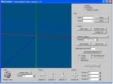
4.3 Snapshot of Cloud Macrostructure Editor 70

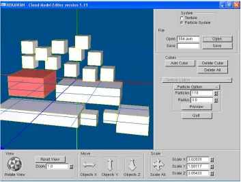
4.4 Using 17 cubes for clouds apparent shape 71

4.5 Cloud modeled with 554 particles 73

4.6 Using 23 cubes for clouds apparent shape 73

4.7 Cloud modeled with 615 particles 75

5.1 Test result for efficiency of the algorithm 78

5.4 Performance Test results for System1 81

(10)

5.9 Comparison of Performance Test for 800×600 resolution 87

5.10 Comparison of Performance Test for 1024×768 resolution 87

(11)

LIST OF ABBREVIATIONS

ABBREVIATION DESCRIPTION

AGP Accelerated Graphics Port

API Application Programming Interface CA Cellular Automation

CML Coupled Map Lattice CSG Constructive Solid Geometry GPU Graphical Processing Unit HMD Head Mounted Display PDE Partial differential Equation VE Virtual Environment

(12)

LIST OF APPENDICES

APPENDIX TITLE PAGE

(13)

CHAPTER I

INTRODUCTION

1.1 Introduction

If clouds were the mere result of the condensation of vapor in the masses of atmosphere which they occupy, if their variations were produced by the movements of the atmosphere alone, then indeed might the study of them be deemed an useless pursuit of shadows, an attempt to describe forms which, being the sport of winds, must be ever varying, and therefore not to be defined. But the case is not so with clouds.

(14)

Clouds are a frequently observed natural phenomenon. They are estimated to cover between 60 and 70 % of the globe at any given time. At most locations on earth some clouds will occur on every single day. Clouds exist in a great variety of forms and on a large range of both temporal and spatial scales. Individual small cumulus clouds for instance cover a few hundred meters in the horizontal and vertical and normally have a lifetime of less than an hour. In contrast the vast, virtually ubiquitous stratocumulus decks covering the eastern parts of the subtropical oceans have a horizontal extent of several hundred kilometers, while being no more than a few hundred meters thick. The processes involved in the formation and dissipation of clouds span an even larger range of scales from micrometers for the condensation of individual droplets to thousands of kilometers for cloud formation in frontal systems associated with mid-latitude baroclinic systems (Christian, 2000).

An analysis of satellite observations shows that about half of the earth's clouds extend above the freezing level and, therefore, are capable of ice production. The clouds, however, do not glaciate instantly as they are exposed to negative temperatures. Mixed phase clouds are commonly observed at temperatures down to

-20°C and below. Nucleation of ice crystals in clouds may occur either by homogeneous freezing of drops or by heterogeneous nucleation on ice nuclei. The former process is believed to be important at temperatures below about -40°C. This process is essential for cirrus formation but its effects may be neglected for most low and middle tropospheric clouds in mid-latitudes (Mikhail, 1997).

(15)

forecast to include a prediction of the occurrence and type of clouds and precipitation. Just as importantly, the desire to estimate the future evolution of our planet's climate requires knowledge about clouds. This is due to their strong interaction with the radiative fluxes whose modification through changes in the atmospheric composition is of considerable concern.

Clouds are a ubiquitous feature of our world. They provide a fascinating dynamic backdrop to the outdoors, creating an endless array of formations and patterns. As with stars, observers often attribute fanciful creatures to the shapes they form, but this game is endless, because unlike constellations, cloud shapes change within minutes. Beyond their visual fascination, clouds are also an integral factor in Earth’s weather systems. Clouds are the vessels from which rain pours, and the shade they provide can cause temperature changes below. The vicissitudes of temperature and humidity that create clouds also result in tempestuous winds and storms. Their stunning beauty, physical and visual complexity, and pertinence to weather have made clouds an important area of study for meteorology, physics, art, and computer graphics (Harris, 2003).

Cloud realism is especially important to flight simulation. Nearly all pilots these days spend time training in flight simulators. To John Wojnaroski, a former USAF fighter pilot and an active developer of the open-source FlightGear Flight Simulator project (FlightGear, 2003), realistic clouds are an important part of flight that is missing from current professional simulators.

One sensation that clouds provide is the sense of motion, both in the simulation and in real life. Not only are clouds important, they are absolutely essential to give the sky substance. Like snowflakes, no two clouds are alike and when you talk to folks involved in soaring you realize that clouds are the fingerprints that tell you what the air is doing.

(16)

clouds would grow and disperse as real clouds do, get blown by the wind, and move in response to forces induced by passing aircraft. Simulated clouds should be realistically illuminated by direct sunlight, internal scattering, and reflections from the sky and the earth below. Previous real-time techniques have not provided users with such experiences.

Clouds have fascinated and vexed computer graphics researchers for many years. The visual appearance of clouds is very complex and extremely varied, yet it is very easy to recognize an "incorrect" cloud model, probably because we see clouds in one form or another every day (Gustav, 1999).

1.2 Motivation

Clouds remain one of the most significant challenges in the area of modeling natural phenomena for computer graphics and it has been a challenge for nearly twenty years. This has made the simulation of various natural phenomena one of the important research fields in computer graphics. Aspects such as sky, clouds, water, fire, trees, smoke, terrains, desert scenes, snow and fog play an important role for creating realistic images of natural scenes. In particular, clouds are indispensable for creating realistic images of natural scenes, outdoor scenes, flight simulators, space flight simulators, visualization of the weather information, creation of realistic clouds from satellite images, simulation of surveys of the earth, earth viewed from outer space, film, art and so on. Some of the motivations factors can be summarized as following:

• Clouds are familiar objects in everyday life, it is desirable to simulate them effectively for the applications, such as entertainment, advertising, and art etc.

(17)

• Realistic cloud simulation would also be an effective tool in the field of

meteorology.

• Indeed, it is reasonable to say that we want to simulate these beautiful natural features simply because they are there.

1.3 Problem Background

There are two important issues for synthesizing photo-realistic images of all natural phenomena including clouds. These are modeling and rendering. Generally, the modeling process includes the creation of shapes of objects, their dynamics (motion/movement) and their physical properties such as surface reflectance. This is however not an easy task for objects such as clouds, smoke and sand dunes (Nishita and Dobashi, 2001). Rendering is the process of generating images by calculating colors for every pixel. The ray-tracing algorithm is often employed for generating images including the sky, clouds, smoke, desert scenes, and the atmospheric effects. Although the ray-tracing algorithm can create extremely realistic images, the computation time is very long.

(18)

Stam and Fiume (1991) have developed a simple method for modeling clouds. In their method, a user specifies density values at several points in three-dimensional space. Then the density distribution of the clouds is obtained by interpolating the specified density values. Although this method can create realistic clouds, it is impractical for creating large-scale clouds viewed from space. Methods for modeling a set of clusters of clouds have also been developed. Ebert et al. (1998) created realistic images of typhoons by the procedural approach. Nishita et al. (1996) have modeled clouds to generate realistic images of the earth viewed from space. In both these methods, however, clouds are simply modeled by applying two-dimensional fractals. The color and shape of clouds change depending on both the viewpoint and the position of the sun. These methods cannot simulate such effects.

The physically based techniques attempt to simulate the meteorological processes that create clouds and the interaction between light and cloudy air (Kajiya and Herzen, 1984; Stam and Fiume, 1991, 1993; Harris et al., 2003).Kajiya and Herzen (1984) used a simple method based on Partial Differential Equations (PDE) to generate cloud data sets for their ray-tracing algorithm. Dobashi et al. (2000) used a simple cellular automata model of cloud formation to animate clouds offline. Miyazaki et al. (2001) extended this to use a coupled map lattice model based on atmospheric fluid dynamics. Overby et al. (2002) described another physical model that, like ours, is based on the stable fluid simulation of Stam (1999). Harris et al. (2003) presented a method most similar to the work by Kajiya and Herzen (1984) and Overby et al. (2002). He implements simulation, dynamics and radiometric entirely on programmable floating-point graphics hardware to get real time simulation. It seems, however, this method is not applicable for large-scale clouds as required by games and flight simulator applications running on desktop machines.

(19)

a slow offline process, where artists manipulate low-complexity avatars as placeholders for the high quality simulation results. With this method, fine tuning the results becomes a very slow, iterative process, where tweaking physical parameters may have no observable consequence or give rise to undesirable side-effects, including loss of precision and numeric instability. Unpredictable results may be introduced from approximations in low-resolution calculations during trial renders. These physics-based interfaces can also be very cumbersome and non-intuitive for artists to express their intention and can limit the animation by the laws of physics.

Clouds consist of small particles and it is very difficult to define their definite shapes. The simulation of their dynamics (movement) is also a difficult task, since their shape changes continuously with time. Therefore, a lot of modeling methods have been developed to address this problem. Using these methods, however, obtaining realistic-looking shapes and motion is very time consuming. For example, the rendering of clouds and smoke requires the integration of the intensity of light scattered by small particles along the viewing ray. On the other hand, the processing speed of graphics hardware has become faster and faster recently. In addition, high performance graphics hardware is available even on low-end PCs. These facts have encouraged researchers to develop hardware-accelerated methods for rendering realistic images (Ofek and Rappoport, 1998; Heidrich and Seidel, 1999; Stam, 1999; Cabral et al., 1999).

After efficiently computing the dynamics and illumination of clouds, there remains the task of generating a cloud image. The translucent nature of clouds means that they cannot be represented as simple geometric “shells”, like the polygonal models commonly used in computer graphics. Instead, a volumetric representation must be used to capture the variations in density within the cloud. Rendering such volumetric models requires much computation at each pixel of the image. This computation can result in excessive rendering times for each frame.

(20)

dimensional density map, which describes the density of the water vapor the object consists of. The density-map is rendered by means of a volume renderer, which takes into account the specific scattering of light-rays, caused by tiny water droplets inside the object. Physical-based simulation, however, demands a high computational cost and is impractical for real time applications. Even on today’s fastest processors, rendering times of about a few minutes per image are common.

Procedural modeling techniques provide simple and efficient methods to simulate natural phenomena and give visually convincing results. Such techniques provide an abstraction of model, encode classes of objects, and allow high-level control and specification of the model. The goal of these modeling techniques is to provide a concise, efficient, flexible, and controllable mechanism for specifying and animating models of complex objects and natural phenomena. Code segments or algorithms are used to abstract and encode the details of the model instead of explicitly storing vast numbers of low-level primitives. The use of algorithms provides great flexibility, and allows amplification of efforts through parametric control - a few parameters to the model yield large amounts of geometric details.

Particle system is one of the procedural techniques. Particle systems are most commonly used to represent natural phenomena such as fire, water, clouds, snow, rain, grass, and trees. A particle-system object is represented by a large collection of very simple geometric particles that change stochastically over time. Particle systems do use a large database of geometric primitives to represent natural objects, but the animation, location, birth, and death of the particles representing the object are controlled algorithmically. The procedural aspect and main power of particle systems allow the specification and control of this extremely large cloud of geometric particles with very few parameters. Besides the geometric particles, a particle system has controllable stochastic particle animation procedures that govern the creation, movement, and death of the particles. These animation procedures often include physically based forces to simulate effects such as gravity, vorticity, conservation of momentum, and energy.

(21)

easily modeled with the particle systems. Particle systems are a simple and efficient method for representing clouds. Cloud model assumes that a particle represents a roughly spherical volume in which a Gaussian distribution governs the density falloff from the center of the particle. Each particle is made up of a center, radius, density, and color. Good approximations of real clouds can be achieved by filling space with particles of varying size and density. Clouds can very easily be built by filling a volume with particles, or by using an editing application that allows placing particles and building clouds interactively. The randomized method is a good way to get a quick field of clouds. Virtual reality applications such as flight simulators have pre-designed levels and require fine control over all details of the scene. Providing an interactive editor allows producing beautiful clouds tailored to the needs.

1.4 Problem Statement

This research focuses on the development of a technique that can be used for synthesizing cloud images in an interactive way. Particles system is used to model these fuzzy objects.

The following research questions are addressed to solve the problem:

a) How efficient is particle system with randomized method for synthesizing cloud images?

b) How can interactive-ness be employed for cloud modeling?

1.5 Objectives of the Study

(22)

cloud shape modeling problem. This research also aims to achieve the following objectives:

a) To investigate, analyze and formulate an appropriate technique for modeling.

b) To define an appropriate mathematical model for the deformation of the physically based cloud motion.

c) To construct a software library for modeling the cloud with the motion analysis.

1.6 Importance of the Study

This study is conducted particularly to construct a randomized based model in solving cloud shape modeling problem. In general, this study introduces a technique consisting of a randomized based algorithm by making use of particles system for modeling cloud shapes and an interactive editor application – cloud macrostructure editor.

The whole research can be divided into two parts. The first part of the research consists on development of a randomized based algorithm using particles system that can fill cloud space by placing particles at random positions to model microstructure of the clouds. The second part deals with the development of an interactive editor application – cloud macrostructure editor, which can be used to model apparent shapes of clouds interactively.

(23)

1.7 Scope of the Study

The scope of the research conducted in this study can be summarized as

follows:

a) In a real system, the number of particles keeps on changing with the passage

of time. Some particles die from the system and at the same time some new

particles are born in the system. For simplicity, the number of particles is

considered as constant in this research i.e., no particle is born and no particle

dies with the passage of time.

b) In reality, each particle may not resemble the other particles and particles

may have different shapes. This research has considered a roughly spherical

volume for each particle for simplicity.

c) Particles in a system are free to move and continuously change their position

as they move along the atmosphere. In this research, each particle has a static

position as this research does not focus on study of cloud dynamics. So

particle do not move in any direction along the atmosphere.

1.8 Thesis Contributions

In this thesis, particles systems are used to model clouds and then synthesize

cloud images by making use of proposed algorithm based on randomized method

that fills the cloud volume with particles randomly. It provides an applicable

platform for the efficient and interactive synthesis of cloud images.

In general, the major contribution described in this thesis can be summarized

as follows:

a) Development of cloud shape modeling algorithm based on randomized

(24)

b) Development of an interactive cloud editing application – cloud macrostructure editor, to model cloud shapes in an interactive way. This approach provides control over number of particles in a particular cloud area and control over size of the particles.

c) Application of cloud macrostructure editor to test interactive-ness of the randomized algorithm for modeling cloud shapes.

1.9 Thesis Organization

This section presents how this thesis is organized. The main structure of the

thesis consists of introduction, literature review, methodology, design, results,

discussion and conclusions in chapters described as below.

Chapter I: Introduction. This chapter introduces the research topic consisting of

various sections i.e. Introduction, Motivation, Problem Background, Problem

Statement, Objectives of the Research, Importance of the Study, Scope of the Study,

Thesis Contributions and Thesis Organization.

Chapter II: Cloud Modeling. This chapter presents current studies in the area of

cloud modeling problem and evaluates the advantages and disadvantages of the

existing solutions.

Chapter III: Particle Systems. This chapter discusses the basics of the particle

system.

Chapter IV: Randomized Particle Algorithm. Definition of the problem addressed

in this research and model formulation are presented in this chapter. Proposed

(25)

Chapter V: Results and Testing. Results of the experiments are summarized and

discussed in this chapter.

Chapter VI: Discussion and Conclusions. This final chapter discusses the strength

and weaknesses of the thesis. This chapter also suggests the future work that can be

done for the extension of the proposed technique. Finally, this chapter concludes the

(26)

CHAPTER II

CLOUD MODELING

2.1 Introduction

Throughout the history of computer graphics, advances have been driven by the quest for visual realism. This quest for visual realism encompassed all aspects of image creation from object definition to object color, illumination and shadowing. For example, early models for representing objects used polygonal meshes. These early polygonal models for representing objects were not used to represent abstract artistic shapes; they were model, of actual objects. Spline patch models were later used for object modeling to more accurately represent cured surfaces in the real world. Early rendering systems rendered faceted shaded, flatly illuminated, alias-prone images. Techniques were then developed by Gouraud and Phong to approximate curved surfaces from polygonal models (Rogers and David, 1985). The illumination models for these objects have also greatly improved from simple Larnbertian models to complex illumination models using radiosity, ray tracing and Cook-Torrance illumination models (Ebert, 1996).

(27)

A survey of previous work on clouds would be incomplete without a description of the variety of methods that have been used in computer graphics to synthesize the images of various natural phenomena including clouds. The rest of this introductory chapter will review advances in creating state-of-the-art images in computer graphics. The use of texture mapping techniques for modeling the surface attributes of objects will be discussed, followed by a discussion on various techniques used for cloud modeling and rendering.

2.2 Texture Mapping Techniques

Texture mapping is a technique for simulating the surface characteristics of an object. This, technique was originally proposed by Catmull in 1974 (Rogers and David, 1985) and is still an important technique for creating realistic images. Texture mapping varies the surface characteristics of an object through the use of mathematical functions, or two-dimensional or three-dimensional tables. This technique has been used to modulate many surface characteristics, including color, roughness, reflection, transparency and even the actual surface geometry (displacement mapping).

Texturing is commonly used in applying a two-dimensional image onto an object to produce a color pattern on the object. Examples of this include creating a label on a wine bottle and the woven fabric color pattern on a sofa.

This technique is also commonly used to simulate bumps, wrinkles, and imperfections on the surface of objects by modifying the normal to the surface of the object. This helps in creating realistic images by reducing the smooth “antiseptic” quality of computer-generated images. Scratches in a table, the winkles on the surface of an orange and the bumps in a stucco wall can all be simulated with two-dimensional texturing of surface normals (bump mapping).

(28)

mapping in that the actual geometry of the surface is modulated (on displaced) instead of just the normal to the surface. Displacement mapping solves two problems that occur with bump mapping, smooth silhouettes and smooth intersections. In bump mapping, the silhouette of the object will not show the effects of' the bump mapping, since the normal vector is just perturbed. The actual geometry of the silhouette (and the entire object) remains unchanged. The intersection of two bump mapped objects will also not show the effects of the bump mapping for the same reason. However, with displacement mapping, the geometry of the object is actually changed, so these problems will not occur.

Displacement mapping and other types of texture mapping are incorporated as follows into the rendering process. Texture mapping normally occurs just before the illumination calculations are performed to determine the final color of the surface element. Texture mapping of surface color, surface normal vector, surface reflection, and other surface illumination parameters is performed just prior to the illumination calculation to determine the final color of this surface element. Texture mapping of surface transparency normally occurs just prior to the combination of this surface element with the surface element behind it. In most rendering systems, displacement mapping needs to be performed before the hidden surface algorithm and actual changes the geometric representation of the object. In most rendering algorithm, texturing is only applied to the visible points on the surface of the object (after the hidden surface calculations). To avoid perspective distortions in the texture, the object space location of the visible point on the surface of the object is usually used in the texture mapping calculation. Different mapping algorithms will be discussed in the following subsections.

2.2.1 Two-Dimensional Texturing

(29)

two-space. This value is t hen used for the particular surface characteristic of the point P on the object. Two-dimensional texturing was originally used in modeling the surface color of objects. Blinn et al. (1976) extended texture mapping to modulate the specular and reflection characteristics of objects. Blinn (1978) further extended texturing to modulate the normal vector of surfaces as a way of simulating bumps and wrinkles on objects. Finally, Cook (1984) suggested using two-dimensional texturing to manipulate all aspects of the illumination of an object, including surface displacement and shadowing.

There are several techniques for mapping the point into this two-dimensional texture space. For a survey of different mapping techniques, see (Heckbert and Paul, 1986). These techniques can be classified into two different classes of mapping techniques. The first class maps each polygon or patch of the object into the entire two-dimensional space. Therefore, using this class of mapping technique repeats the texture on each polygon or patch of the object. Within this class of mappings, two different mapping techniques are commonly used. The first mapping technique is referred to as inverse bilinear interpolation (Heckbert and Paul, 1986). This technique first, uses the inverse perspective transformation to transform the image space location of the point on the surface of the object into object space. Then, the point in object space is mapped into the texture definition space through the use of inverse bilinear interpolation. The second technique uses simple bilinear interpolation in screen space, where the location of the point in screen space is used in the texture mapping, and not the location of point in object space, as in the previous technique. This technique, however, suffers from perspective distortion. A more detailed description of these techniques can he found in (Heckbert and Paul, 1986).

(30)

technique, the user assigns texture space coordinates with each vertex of a polygon (or control point of a patch). Then, during scan conversion, these texture space coordinates are simply linearly interpolated to determine the texture space coordinate for each visible point on the surface of the object.

The mapping of each pint on the surface of a three-dimensional object into the two-dimensional texture space creates many problems in the resultant appearance of the texture applied to the object. The two-dimensional texture may suffer distortions when applied to the three-dimensional object. For example, when a simple spherical projection is used to map a two-dimensional texture onto an object, the texture is normally compressed near the poles and stretched near the equator of the object. Another problem caused by the texture mapping is discontinuities at the seams of the texture applied to the object. A seam is where two separate sides of the texture map meet when the texture is applied to the object. Discontinuities can occur at the seams for two reasons. First, the values in the texture map at the two edges that meet may not be the same. Second, the scale can change abruptly at the seams because of the mapping technique. The surface area that each section of the texture map occupies on opposite sides of the seam may be different because of the mapping. Blurring or averaging of values at the seams can be used to solve this problem (Burt et al., 1983).

A few techniques have also been proposed to solve the distortion problem. The first technique is referred to as two-part texture mapping (Bier and Kenneth, 1986). In this technique, the texture is first projected onto an intermediate dimensional shape. Then the texture is mapped from the intermediate three-dimensional shape onto the final object. The choice of the separate parts of the mapping allows for choosing a combination of techniques that minimize distortion for the particular object.

(31)

mapping to apply the texture to the object. Problems with this technique include the possibility of introducing discontinuities into the texture applied to the image and loss of texture when applied to the object (parts of the texture map may not be applied to the object). This technique is used to reduce distortion and scale changes when the texture map is applied to the object. It still does not solve the problem with seams.

2.2.2 Three-Dimensional Texturing - Solid Texturing

In 1985, Gardner (1985), Peachey and Darwyn (1985) and Perlin (1985) all independently suggested extending two-dimensional texturing to three-dimensional texturing or solid texturing. Solid texturing differs from two-dimensional texturing in that solid texturing maps each point on the surface of an object to a three-dimensional texture space as opposed to a two-three-dimensional texture space. The location of the point in this three-dimensional “solid space” is used in calculating the value for modulating the surface characteristic of' the point on the object.

Solid texturing is incorporated into the viewing algorithm in a manner similar to two-dimensional texture mapping. As in two-dimensional texturing, the three-dimensional screen space location of each visible point on the surface of the object is mapped back to object space. The main difference is that then this three-dimensional object space location is used by the solid texturing functions to determine the value of the corresponding screen location, as opposed to the two-dimensional location used in two-dimensional texturing.

Gardner (1985) uses three-dimensional texturing for simulating clouds. This technique is used as a model for clouds by using Fourier synthesis to control the transparency of hollow ellipsoids. Figure 2.1 shows complex clouds modeled by Gardner (1985) by making use of linked ellipsoids.

(32)

Figure 2.1: Complex clouds modeled by linked ellipsoids (Gardner, 1985)

Peachey and Darwyn (1985) and Perlin (1985) both proposed solid texturing for controlling the color patterns of objects. They both also used solid texturing as a model for simulating objects carved from solid materials. In solid texturing, the texture is determined from evaluating three-dimensional functions based on the location of each point on the surface of an object in the solid texture Space. Therefore, solid texturing is an extremely powerful technique for simulating objects carved from solid materials such as wood, marble, granite, and other stone materials.

Peachey and Darwyn (1985) use both three-dimensional functions and projected two-dimensional images for defining his three-dimensional textures. Peachey has suggested several functions, which can be used to create interesting three-dimensional textures. By randomly placing spheres of random size throughout a solid space, he simulates materials in which bubbles of one material are captured in the solidification of another material. To simulate wood, Peachey uses concentric cylinders of light and dark colors aligned along an arbitrary axis in three-space. Peachey simulates marble through placing starting locations for veins within the solid space. The direction of the veins is then controlled through the use of sinusoidal functions. The diameter of the cross-section of the veins is also controlled by more sinusoidal functions.

(33)

able to create very realistic images of marble, fire, water, and block glass. Details can be found in (Perlin, 1985).

Solid texturing solves some problems of two-dimensional texturing. Since solid texturing uses an affine mapping from the three-dimensional object space to the three-dimensional texture space (normally scale and translation transformations), there is no distortion of the texture when it is to the object. In two-dimensional texturing where a two-dimensional image is mapped onto a complex three-dimensional manifold, distortion and mapping of the texture applied to the object can occur. Solid texturing avoids these problems.

2.3 Simulating Complex Geometry

There have been many approaches to modeling the complex geometry of objects in our environment. Polygonal and patch models were the first models used. Constructive solid geometry (CSG) models were introduced later. More recent models can be categorized as either particle systems or procedural models.

2.3.1 Polygonal and Patch Modeling

(34)

example, the silhouette of the object is still polygonal and so is the line of' intersection of two polygonal objects.

Spline surface patches solve some of the problems with polygonal patch models, since they are an actual curved surface model useful for simulating smooth surfaces in our environment. Surface patch models have been extended to formulations that are easier to control and they have advantages over earlier formulations, such as hierarchical Spline models. Forsey and Bartels (1988) have created a hierarchical spline model that allows for uneven spacing of control points to provide an efficient formalization for objects that have areas of varying degrees of surface details.

Both polygonal and surface patch models are usually created by digitizing a real world model, or using an interactive system to create the model.

2.3.2 Constructive Solid Geometry Models

(35)

Calculating the boundary representation from the CSG models requires extensive computations. Second, some shapes are not easily described as Boolean operations on simple shapes.

2.3.3 Particle Systems

A more recent approach to modeling complex geometric objects is particle systems. Reeves (1983) originated the use of particle systems. Particle systems have mainly been used for modeling natural phenomena, such as smoke, cloud, fire, trees, and water where the intricate detail of the phenomena is represented by a large collection of particles. Particle systems normally involve the use of a large number of small spherical particles. The animation of these particles is controlled through the use of procedures, which simulate the specific natural object, such as fire. The rendering of particle systems normally uses a simple constant shading model and often the color of the particle is determined by its three-dimensional location in space. For example, in Reeves' fire simulation (Reeves, 1983), the color of the particle is determined by its elevation from the base of the fire.

Particle systems have several advantages over patch and polygonal models. Particle systems normally use simple spheres for representing the geometry of the object or phenomenon, instead of complex patch or polygonal models. Therefore, the rendering system only needs to handle simple spherical models. The particle system rendering process also usually uses constant flat shading for the illumination of the particles, which is much simpler and quicker than normal illumination algorithms used for patch and polygonal models.

(36)

2.3.4 Procedural Modeling

Many different, modeling techniques can he termed procedural modeling. Fractal synthesis (Mandelbrot, 1982), Fourier synthesis (Gardener, 1985), hypertextures (Perlin and Hoffert, 1989), L-systems (Prusinkiewicz et al., 1988), volume density functions (Ebert and Parent, 1990), and inverse particle systems can all be considered to be procedural models. Procedural modeling uses algorithms to represent the geometry of objects. Most, physically based modeling techniques are also procedural modeling techniques, for example Kajiya’s cloud modeling technique (Kajiya and Herzen, 1984).

Procedural modeling techniques have many advantages over polygonal and patch modeling techniques. The procedural model is evaluated during the rendering process to determine the geometry of the object / phenomena. Usually, the model is evaluated at the resolution of image rendering. Therefore, the models provide the needed amount of detail without introducing high frequency details, which will result in aliasing artifacts. Secondly, complex shapes can be represented with very little data storage space. For instance, a fractal mountain can be represented with a procedure of less than 50 lines of C language code; whereas, to achieve an equivalently detailed polygona1 model might require 50,000 polygons (Ebert, 1996). Because of this, procedural modeling techniques are often used to represent objects of very high degrees of detail such as natural phenomena.

(37)

2.4 Modeling Natural Phenomena

Natural phenomena are some of the hardest things to model in computer graphics. Modeling phenomena such as mountains, trees, plants, fire, water, clouds, and smoke have inspired much research in computer graphics. Realistic models of these phenomena, however, still elude current computer graphics techniques. The complex intricate geometry and motion of these phenomena make them very difficult to model. Some natural phenomena, such as mountains, trees, and plants have intricate rigid shapes, while others; such as clouds, fire, and water have intricate amorphous shapes. Most models for natural phenomena can he classified as fractals, particle systems, or other types of procedural models.

2.4.1 Modeling Terrain and Vegetation

Most approaches to modeling terrain have used a fractal modeling approach (Miller, 1986). Mandelbort and Musgrave (Musgrave et al., 1989) have done much work on the modeling of terrain using fractals. Recent work has included modeling terrain with fractals and then simulating the natural erosion processes that affect terrain to create a more realistic model (Musgrave et al., 1989).

There has been a wider range of techniques used to model vegetation. Iterated functions systems (Demko et al., 1985), fractals, particle systems (Reeves and Blau, 1985) and L-systems (Prusinkiewicz et al., 1988) have all been used to model plants and trees. Very realistic images of plants have recently been produced through the use of L-systems

2.4.2 Modeling Fire and Water

(38)

controlling the height of the surface of the water (Max, 1981). This model had many problems, including its inability to simulate breaking or curling waves since there can only be one height value for each x-y location. 1986 and 1987 saw a flurry of research in modeling ocean waves (T'so and Barsky, 1987; Fournier and Reeves, 1986; Peachey, 1986). Some of these models provided mom physically based models that simulated breaking waves and even spray from breaking waves created by particle systems (Fournier and Reeves, 1986). More recently, Kass and Miller (1990) have developed a model based on wave equations that even allows for the net transport of water volume. The main drawback with their approach is that they again use a height field, so they cannot simulate cresting or breaking waves.

The modeling of fire has received very little attention compared to the modeling of water. The main approach to modeling fire has been the use of particle systems (Reeves, 1983; Sims, 1990).

2.4.3 Modeling and Animating Gaseous Phenomena

The rendering of scenes containing clouds, fog, atmospheric dispersion effects, and other gaseous phenomena has received much attention in the computer graphics literature. Several papers deal mainly with atmospheric dispersion effects (Willis, 1987; Nishita el al., 1987; Rushmeier and Torrance, 1987), while many cover the illumination of these gaseous phenomena in detail (Blinn, 1982; Kajiya and Herzen, 1984; Max, 1986; Kass and Miller, 1990). Most authors have used a low albedo reflection model, while a few, B1inn (1982), Kajiya and Herzen (1984), and Rushmeier and Torrance (1987), discuss the implementation of a high albedo model.

A low albedo reflectance model assumes that secondary scattering effects are negligible, while a high albedo illumination model calculates the secondary and higher order scattering effects.

(39)

layers of constant densities. This allows for a very limited geometry for the gases. Voss (1983) uses fractals and Max (1986) uses height fields for modeling the geometry of clouds. Kajiya and Herzen (1984) use a physically based model for clouds, which simulates water vapor, heat flow, wing, etc to form a physical model for clouds. However, the resulting images are not very realistic. Gardner (1985) uses hollow ellipsoids to model the geometry of clouds. He controls the transparency of hollow ellipsoids through the use of Fourier synthesis. To form larger cloud formations, he combines many different ellipsoids to form cloud groups. The main problem with his approach is that it is not a true three-dimensional model for the clouds, so accurate cloud shadowing is impossible. Another problem is that once you enter a cloud, you can clearly see that it is a simple hollow object and not a full three-dimensional cloud volume.

Ebert and Parent (1990) use turbulent flow based functions to model the density of a variety of gases. These functions are based on Perlin’s visual simulation of turbulent flow (Perlin, 1985) and are similar to the idea of hypertextures (Perlin and Hoffert, 1989). This model is a true three-dimensional model for the geometry of gases and provides realistic results. This technique seems to provide more realistic results than most previous efforts by providing visually realistic renderings and animations of gaseous phenomena and the shadows they cast. These techniques are based on a visual simulation of turbulent flow, so it is a visual simulation of the turbulent processes that determines the geometry of gaseous phenomena. These techniques can also be extended to use a physically based turbulent flow model and can be very efficient when simplifying assumptions are made. This approach will be discussed in more detail later in this dissertation.

2.5 Modeling Fuzzy Objects

(40)

methods that have been used to model and render clouds: particle systems, metaballs, voxel volumes, procedural noise, and textured solids. Note that these techniques are not mutually exclusive; multiple techniques have been combined with good results.

2.5.1 Particle Systems

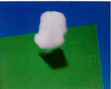
Particle systems model objects as a collection of particles—simple primitives that can be represented by a single 3D position and a small number of attributes such as radius, color, and texture. Reeves (1983) introduced particle systems in as an approach to modeling clouds and other “fuzzy” phenomena, and described approximate methods of shading particle models in (Reeves and Blau, 1985). Particles can be created by hand using a modeling tool, procedurally generated, or created with some combination of the two. Particles can be rendered in a variety of ways. Harris and Lastra (2001) modeled static clouds with particles and rendered each particle as a small texture sprite (or “split” (Westover, 1990)). The details of this technique can be found in (Harris and Lastra, 2001). Figure 2.2 shows clouds modeled by Harria and Lastra (2001).

Figure 2.2: Shading with multiple forward scattering. (Harris and Lastra, 2001)

(41)

2.5.2 Metaballs

Metaballs (or “blobs”) represent volumes as the superposition of potential fields of a set of sources, each of which is defined by a center, radius, and strength (Blinn, 1982a). These volumes can be rendered in a number of ways, including ray tracing and splatting. Alternatively, isosurfaces can be extracted and rendered, but this might not be appropriate for clouds. Nishita et al. (1999) used metaballs to model clouds by first creating a basic cloud shape by hand-placing a few metaballs, and then adding detail via a fractal method of generating new metaballs on the surfaces of existing ones (Nishita et al., 1996). Dobashi et al. (1999) used metaballs to model clouds extracted from satellite images. In Dobashi et al. (2000), clouds simulated on a voxel grid were converted into metaballs for rendering with splatting. The figure 2.3 shows a snapshot of clouds formed around mountains, as modeled by Dobashi et al. (2000).

Figure 2.3: Cloud formation around mountains (Dobashi et al., 2000)

2.5.3 Voxel Volumes

(42)

represented as voxel volumes (Levoy, 1988; Westover, 1990; Wilson et al., 1994; Cabral et al., 1994; Kniss et al., 2002). Voxel grids are typically used when physically-based simulation is involved. Kajiya and Herzen (1984) performed a simple physical cloud simulation and stored the results in a voxel volume which they rendered using ray tracing. Figure 2.4 shows clouds rendered by Kajiya and Herzen (1984).

Figure 2.4: Cloud rendered by ray tracing (Kajiya and Herzen, 1984)

Dobashi, et al. (1998) simulated clouds on a voxel grid using a cellular automata model similar to Nagel and Raschke (1992), converted the grid to metaballs, and rendered them using splatting (Dobashi et al., 2000). Miyazaki et al. (2001) also performed cloud simulation on a grid using a method known as a Coupled Map Lattice (CML), and then rendered the resulting clouds in the same way as Dobashi et al. Overby et al. (2002) solved a set of partial differential equations to generate clouds on a voxel grid and rendered them using SkyWorks rendering engine (Harris and Lastra, 2001).

2.5.4 Procedural Noise

(43)

cloud volumes (Lewis, 1989; Perlin, 1985). Ebert has done much work in modeling “solid spaces” using procedural solid noise, including offline computation of realistic images of smoke, steam, and clouds (Ebert and Parent, 1990; Ebert, 1997; Ebert et al., 2002). Ebert modeled clouds using a union of implicit functions. He then perturbed the solid space defined by the implicit functions using procedural solid noise, and rendered it using a scan line renderer. Schpok et al. (2003) recently extended Ebert’s techniques to take advantage of programmable graphics hardware for fast animation and rendering. Figure 2.5 shows volumetric implicit turbulent cloud modeled by Ebert (1997).

Figure 2.5: Volumetric Implicit Turbulent Cloud (Ebert, 1997)

2.5.5 Textured Solids

(44)

render clouds composed of multiple ellipsoids (Elinas and Sturzlinger, 2001). Figure 2.6 shows clouds modeled by Elinas and Sturzlinger (2001) using 30 ellipsoids.

Figure 2.6: Cloud constructed from 30 ellipsoids (Elinas and Sturzlinger, 2001)

2.6 Cloud Dynamics Simulation

Cloud simulation has been of interest to meteorologists and atmospheric scientists since the advancement in high performance computing, but it has only recently drawn much interest from the computer graphics community. Scientific simulations of clouds and weather are typically very complex, requiring many hours of computation to simulate a relatively short time of cloud development.

(45)

in the rotational motion of the clouds (Steiner, 1973). Three-dimensional cloud simulation has progressed since then.

Simulations from atmospheric physics are too expensive for computer graphics applications other than scientific visualization. Because they are used to understand our atmosphere and weather, many of them include a high level of detail that is not visible in nature, including very specific tracking of water state and droplet size distributions, complex microphysics, and detailed fluid dynamics at a variety of scales. If the goal is simply to create realistic images and animations of clouds, much less detailed visual simulations can be used.

Kajiya and Herzen were the first in computer graphics to demonstrate a visual cloud simulation (Kajiya and Herzen, 1984). They solved a very simple set of partial differential equations to generate cloud data sets for their ray tracing algorithm. The Partial differential Equations (PDE) they solved were the Navier-Stokes equations of incompressible fluid flow; a simple thermodynamic equation to account for advection of temperature and latent heat effects; and a simple water continuity equation. The simulation required about 10 seconds per time step (one second of cloud evolution) to update a 10×10×20 grid on a VAX 11/780. Overby et al. described a similar but slightly more detailed physical model based on PDEs (Overby et al., 2002). They used the stable fluid simulation algorithm of (Stam, 1999) to solve the Navier-Stokes equations. The stability of this method allows much larger time steps, so Overby et al. were able to achieve simulation rates of one iteration per second on a 15 × 50 × 15 grid using an 800MHz Pentium III. Harris has implemented a faster and slightly more realistic cloud simulation using programmable floating point graphics hardware (Harris et al., 2003; Harris, 2003).

(46)

clouds in humid cells, but included no mechanism for evaporation. Dobashi et al. added a stochastic rule for evaporation so that the clouds would appear to grow and dissipate. Their model achieved a simulation time of about 0.5 seconds on a 256 × 256 × 20 volume using a dual 500 MHz Pentium III.

In similar work, Miyazaki et al. used a coupled map lattice rather than a cellular automaton (Miyazaki et al., 2001). This model was an extension of an earlier coupled map lattice model from the physics literature. Coupled map lattices (CML) are an extension of CA with continuous state values at the cells, rather than discrete values. Harris et al. have done work on performing CML simulations on programmable graphics hardware (Harris et al., 2002). The CML of Miyazaki et al. used rules based on atmospheric fluid dynamics, including a rule used to approximate incompressibility and rules for advection, vapor and temperature diffusion, buoyancy, and phase changes. They were able to simulate a 3–5 s time step on a 256 × 256 × 40 lattice in about 10 s on a 1 GHz Pentium III.

2.7 Light Scattering and Cloud Radiometry

Some of the earliest work on simulating light scattering for computer graphics was presented in (Blinn, 1982b). Motivated by the need to render the rings of Saturn, Blinn described an approximate method for computing the appearance of cloudy or dusty surfaces via statistical simulation of the light-matter interaction. Blinn (1982b) made a simplifying assumption in his model—that the primary effect of light scattering is due to reflection from a single particle in the medium, and multiple reflections can be considered negligible. This single scattering assumption has become common in computer graphics, but as Blinn (1982b) and others have noted, it is only valid for media with particles of low single scattering albedo. Blinn (1982b) also simplified the problem by limiting application of his model to plane parallel atmospheres, rather than handling scattering in arbitrary domains.

(47)

of a double integral equation. In practice, researchers either use simplifying assumptions to reduce the complexity of the problem, or perform long offline computations. There are multiple ways to compute light scattering, and many simplifications that can be applied. The previous work in this area can be grouped into five categories: Spherical Harmonics Methods, Finite Element Methods, Discrete Ordinates, Monte Carlo Integration, and Line Integral Methods.

2.7.1 Spherical Harmonics Methods

The spherical harmonics Ylm (θ, φ) are the angular portion of the solution of

Laplace’s equation in spherical coordinates. The spherical harmonics form a complete orthonormal basis. This means that an arbitrary function f(θ, φ) can be represented by an infinite series expansion in terms of spherical harmonics:

∑ ∑∞ = =

=

0 0

)

,

(

)

,

(

l l m m l m l

Y

A

f

θ

φ

θ

φ

(2.1)

The method of determining the coefficients, Alm, of the series is analogous to

determining the coefficients of a Fourier series expansion of a function. If the value of f is known at a number of samples, then a series of linear equations can be formulated and solved for the coefficients. Spherical harmonics methods have been used by (Bhate and Tokuta, 1992; Kajiya and Herzen, 1984; Stam, 1995) to compute multiple scattering.

(48)

scattering of light to the eye was computed, resulting in a cloud image. For multiple scattering, the authors derived a discrete spherical harmonics approximation to the multiple scattering equations, and solved the resulting matrix of partial differential equations using relaxation. This matrix solution replaces the first integration pass of the single scattering algorithm. As mentioned in (Stam, 1995), this method is known as the PN-method in the transport theory literature, where N is the degree of the highest harmonic in the spherical harmonic expansion.

Following Kajiya and Herzen’s lead, two pass algorithms for computing light scattering in volumetric media are now common. Interestingly, (Max, 1994) points out that while Kajiya and Herzen attempted to compute multiple scattering for the case of an isotropic phase function, it is not clear if they succeeded, all of the images in the paper seem to have been computed with the simpler single scattering model.

(49)

2.7.2 Finite Element Methods

The finite element method is another technique for solving integral equations that has been applied to light transport. In the finite element method, an unknown function is approximated by dividing the domain of the function into a number of small pieces, or elements, over which the function can be approximated using simple basis functions (often polynomials). As a result, the unknown function can be represented with a finite number of unknowns and solved numerically.

A common application of finite elements in computer graphics is the radiosity method for computing diffuse reflection among surfaces. In the radiosity method, the surfaces of a scene represent the domain of the radiosity function. An integral equation characterizes the intensity, or radiosity, of light reflected from the surfaces. To solve the radiosity equation, the surfaces are first subdivided into a number of small elements on which the radiosity will be represented by a sum of weighted basis functions. This formulation results in a system of linear equations that can be solved for the weights. The coefficients of this system are integrals over parts of the surfaces. Intuitively, light incident on an arbitrary point in the scene can be reflected to any other point; hence the coefficients are integrals over the scene. In the finite element case, these integrals are evaluated for every pair of elements in the scene, and are called form factors.

(50)

scattering and absorption by the participating medium. Rushmeier and Torrance’s presentation of the zonal method was limited to isotropic scattering media, with no mention of phase functions.

Nishita et al. introduced approximations and a rendering technique for global illumination of clouds, accounting for multiple anisotropic scattering and skylight (Nishita et al., 1996). This method can also be considered a finite element method, because the volume is divided into voxels and radiative transfer between voxels is computed. Nishita et al. made two simplifying observations that reduced the cost of the computation. The first observation was that the phase function of cloud water droplets is highly anisotropic, favoring forward scattering. The result of this is that not all directions contribute strongly to the illumination of a given volume element. Therefore, Nishita et al. computed a “reference pattern” of voxels that contributed significantly to a given point. This pattern is constant at every position in the volume, because the sun can be considered to be infinitely distant. Thus, the same sampling pattern can be used to update the illumination of each voxel. The second observation they made was that only the first few orders of scattering contribute strongly to the illumination of a given voxel. Therefore, Nishita et al. only computed up to the third order of scattering.

2.7.3 Discrete Ordinates

(51)

on the basic method of discrete ordinates by efficiently spreading the shot radiosity over an entire direction bin, rather than along discrete directions. The method achieves a large speedup by handling a whole plane of source elements simultaneously, which reduces the computation time to O(MN log N +M2N) (Harris, 2003).

2.7.4 Monte Carlo Integration

Monte Carlo Integration is a statistical method that uses sequences of random numbers to solve integral equations (Harris, 2003). In complex problems like light transport, where computing all possible light-matter interactions would be impossible, Monte Carlo methods reduce the complexity by randomly sampling the integration domain. With enough samples, chosen intelligently based on importance, an accurate solution can be found with much less computation than a complete model would require. The technique of intelligently choosing samples is called importance sampling, and the specific method depends on the problem being solved. A common application of Monte Carlo methods in computer graphics is Monte Carlo ray tracing. In this technique, whenever a light ray traversing a scene interacts with matter (either a solid surface or a participating medium), statistical methods are used to determine whether the light is absorbed or scattered (for solids, this scattering may be thought of as reflection or refraction). If the light is scattered, the scattered ray direction is also chosen using stochastic methods. Importance sampling is typically used to determine the direction via the evaluation of a probability function.

(52)

ensures that the most significant contributions of scattering are used to determine the intensity. In this way, the technique is similar to the “reference pattern” technique used by (Nishita et al., 1996).

Photon mapping is a variation of pure Monte Carlo ray tracing in which photons (particles of radiant energy) are traced through a scene (Jensen, 1996). Many photons are traced through the scene, starting at the light sources. Whenever a photon lands on a nonspecular surface it is stored in a photon map, a data structure that stores the position, incoming direction, and radiance of each photon hit. The radiance on a surface can be estimated at any point from the photons closest to that point. Photon mapping requires two passes; the first pass builds the photon map, and the second generates an image from the photon map. Image generation is typically performed using ray tracing from the eye. The photon map exhibits the flexibility of Monte Carlo ray tracing methods, but avoids the grainy noise that often plagues them. Jensen and Christensen extended the basic photon map to incorporate the effects of participating media (Jensen and Christensen, 1998). To do so, they introduced a volume photon map to store photons within participating media, and derived a formula for estimating the radiance in the media using this map. Their techniques enable simulation of multiple scattering, volume caustics (focusing of light onto participating media caused by specular reflection or refraction), and color transfer between surfaces and volumes of participating media.

2.7.5 Line Integral Methods

Recently, interest in simulating light scattering has grown among developers of interactive applications. For view-dependent effects and dynamic phenomena, the techniques described in the previous sections are not practical. While those techniques accurately portray the effects of multiple scattering, they require a large amount of computation. For interactive applications, simplifications must be made.

(53)

absorption by the medium is desirable. This requires at least one pass through the volume (along the direction of light propagation) to integrate the intensity of transmitted light. Because methods that make this simplification perform the intensity integration along lines from the light source through the volume may be called line integral methods. Kajiya and Herzen’s original single scattering algorithm is a line integral method. Intuitively, line integral methods are limited to single scattering because they cannot propagate light back to points already traversed.

Dobashi et al. (2000) described a simple line integral technique for computing the illumination of clouds using the standard blending operations provided by computer graphics Application Programming Interface (API) such as OpenGL (Segal and Akeley, 2001). Dobashi et al. (2000) represented clouds as collections of large “particles” represented by textured billboards. To compute illumination, they rendered the particles in order of increasing distance from the sun into an initially white frame buffer. They configured OpenGL blending operations so that each pixel covered by a particle was darkened by an amount proportional to attenuation by the particle. After rendering a particle, they read the color of the pixel at the center of projection of the particle from the frame buffer. They stored this value as the intensity of incident light that reached the particle through the cloud. Traversal of the particles in order of increasing distance from the light source evaluates the line integral of extinction through each pixel. Because pixels are darkened by every particle that overlaps them, this method computes accurate self-shadowing of the cloud. After this first pass, they rendered particles from back to front with respect to the view point, using the intensities computed in the first pass. They configured blending to integrate absorption and single scattering along lines through each pixel of the image, resulting in a realistic image of the clouds. Dobashi

et al. (2000) further enhanced this realism by computing the shadowing of the terrain by the clouds and shafts of light between the clouds.