Space-time block coding with imperfect channel estimation and synchronization

(1)

University of Windsor University of Windsor

Scholarship at UWindsor

Electronic Theses and Dissertations Theses, Dissertations, and Major Papers

2010

Space-time block coding with imperfect channel estimation and

synchronization

Yi Xiao

University of Windsor

Follow this and additional works at: https://scholar.uwindsor.ca/etd

Recommended Citation Recommended Citation

Xiao, Yi, "Space-time block coding with imperfect channel estimation and synchronization" (2010). Electronic Theses and Dissertations. 147.

https://scholar.uwindsor.ca/etd/147

This online database contains the full-text of PhD dissertations and Masters’ theses of University of Windsor students from 1954 forward. These documents are made available for personal study and research purposes only, in accordance with the Canadian Copyright Act and the Creative Commons license—CC BY-NC-ND (Attribution, Non-Commercial, No Derivative Works). Under this license, works must always be attributed to the copyright holder (original author), cannot be used for any commercial purposes, and may not be altered. Any other use would require the permission of the copyright holder. Students may inquire about withdrawing their dissertation and/or thesis from this database. For additional inquiries, please contact the repository administrator via email

(2)

SPACE-TIME BLOCK CODING WITH

IMPERFECT CHANNEL ESTIMATION AND SYNCHRONIZATION

by Yi Xiao

A Thesis

Submitted to the Faculty of Graduate Studies and Research through the Department of Electrical and Computer Engineering

in Partial Fulfillment of the Requirements for the Degree of Master of Application Science at the

University of Windsor

Windsor, Ontario, Canada 2010

(3)

Space-Time Block Coding with Imperfect Channel Estimation and Synchronization by

Yi Xiao

APPROVED BY:

_____________________________________________________ Dr. Robert D. Kent

School of Computer Science, University of Windsor

_____________________________________________________ Dr. Huapeng Wu

Department of Electrical and Computer Engineering, University of Windsor

_____________________________________________________ Dr. Behnam Shahrrava, Advisor

_____________________________________________________ Dr. N. Kar, Chair of Defense

(4)

iii

AUTHOR'S DECLARATION OF ORIGINALITY

I hereby certify that I am the sole author of this thesis and that no part of this thesis has been published or submitted for publication.

I declare that this is a true copy of my thesis, including any final revisions, as approved by my thesis committee and the Graduate Studies office, and that this thesis has not been submitted for a higher degree to any other University or Institution.

(5)

iv

ABSTRACT

Two major challenges of applying Alamouti’s space-time block coding (STBC) [1] to a practical system are the imperfect channel estimation and rough synchronization. Without the full knowledge of channel state information (CSI), the receiver is highly likely to make wrong decisions; on the other hand, without the time alignment of the transmit antennas, the system will suffer from the inter-symbol interference (ISI) [32].

(6)

v

ACKNOWLEDGEMENTS

I want to begin by thanking my advisor, Professor Behnam Shahrrava for his guidance and patience throughout my entire MASc. program of study. It is impossible to finish this thesis without his help. His technical expertise and preciseness in research, together with his warmth and kind personality, has been a model for me to follow. I would also like to express my gratitude to Professor Robert D. Kent, Huapeng Wu and for serving on my graduate committee.

To all my friends, thank you for your friendship, you made my journey in Windsor a much enjoyable and easier one.

(7)

vi

List of Tables

2.1 Transmission Sequence of Four-State STTC. ... 10

(11)

x

List of Figures

1.1 Block Diagram of MIMO System ... 3

2.1 Four-State Space-Time Trellis Diagram. ... 9

2.2 4-PSK Modulation Constellation. ... 9

2.3 Block Diagram of Alamouti’s STBC. ... 14

2.4 The BER Performance of Alamouti’s STBC in Rayleigh Fading Channel. ... 17

3.1 Performance of Alamouti’s STBC under Imperfect Channel Estimation. ... 25

3.2 Cooperative STBC Model with 2 Relay Nodes. ... 27

3.3 Impact of Imperfect Synchronization between 2 Relay Nodes. ... 30

3.4 Performance of Alamouti’s STBC under Imperfect Synchronization. ... 32

5.1 Block Diagram of Alamouti’s STBC System. ... 44

5.2 STBC Transmission with Imperfect Synchronization. ... 63

5.3 Block Diagram of the Proposed Receiver. ... 71

6.1 The BER Performance of Alamouti’s STBC with Perfect Channel Estimation and Synchronization Using L-MMSE Estimator ... 75

6.2 The BER Performance of Alamouti’s STBC with Imperfect Channel Estimation Using Tarokh’s Decision Rule. ... 75

6.3 The BER Performance of STBC under Imperfect Synchronization with and without PIC Detector. ... 77

(12)

xi

6.5 The Impact of Error Propagation (EP) on the BER Performance of PIC Detector. Time Error τ =0.2 , 0.8T T . ... 78

6.6 The BER Performance of Proposed Receiver Compared with Conventional PIC Detector. Time Error β = −5, 0, 5(dB), 2 _0.2

e

σ = . ... 78

(13)

xii

Abbreviations

AS Antenna selection

AWGN Additive white Gaussian noise A&F Amplify-and-forward

BLAST Bell laboratories layered space-time BER Bit error rate

BE-STBC Block-based equalization STBC CSI Channel state information DC Frequency down conversion D&F Decode-and-forward

EP Error propagation FEC Forward error correction ISI Inter-symbol interference LS Least-squares

MSE Mean square error

(14)

xiii MRRC Maximal ratio receiver combining

OFDM Orthogonal frequency-division multiplexing pdf Probability distribution function

PEP Pair-wise error probability PIC Parallel interference cancellation PQO-STBC Power allocated quasi-orthogonal STBC PSK Phase shift keying

QAM Quadrature amplitude modulation QoS Quality of service

(15)

xiv

Notations

a A vector

A A matrix

A Magnitude/ absolute value of A

[ ]

T

⋅ Transpose of a vector or a matrix

[ ]

H

⋅ Hermitian transpose of a vector or a matrix

[ ]

*

⋅ Complex conjugate

( )

−1

A Inverse of matrix A

2

a 2 _H

= a a a

[ ]

E x Statistic average of a random variable x

{ }

var x var

{ }

x =E x⎡ ⎤_{⎣ ⎦}2 −

(

E x

[ ]

)

2

rr

C Covariance matrix of r

sr

C Cross-covariance matrix of sand r

[ ]

p x Probability density function of a random variable x

[ ]

P X Probability of an event X

s

E Average symbol energy

K N

(16)

1

Chapter 1 Introduction

Since 1897, when Guglielmo Marconi first used radio to contact with ships sailing the English channel, new wireless communications methods and services have been evolved remarkably and adopted by people enthusiastically throughout the world. Driven by the transformation of demand from voice telephony service into other services, such as transmission of images, video and data, the telecommunication industry has shifted towards 3G and 4G services. These new services require the wireless systems to have higher data rates, better quality of service (QoS) and coverage, and be deployed in diverse environments. However, unlike wired systems, such as fiber or coaxial cable, whose demands for additional capacity can be fulfilled largely with the addition of new private infrastructure, such as additional optical fiber, cable, routers, and so on, additional wireless capacity cannot be derived from the addition of two major wireless resources: radio bandwidth and transmitter power. Since these two resources are among the most severely limited in the development of modern wireless networks: radio bandwidth because of the very tight situation with regard to useful radio spectrum, and transmitter power because the battery must remain small since the wireless devices must remain simple and portable.

(17)

2

transmitted by diverse ways of electromagnetic wave propagation, such as reflection, diffraction, scattering, and so on. Since most mobile wireless systems operate in urban area, the transmission path between the transmitter and the receiver can vary from simple line-of sight to one that is severely obstructed by buildings and foliage. Due to multipath reflections from various objects, the electromagnetic waves travel along different paths of varying lengths. The interaction between these waves causes multipath fading effect. In additive white Gaussian noise (AWGN) channel, 1-dB improvement in signal to noise ratio (SNR) may reduce the bit error rate (BER) by 90%. In a multipath fading environment, however, 10 dB higher SNR may be needed to achieve the similar amount of reduction of BER.

Given these circumstances, higher data rates can be achieved by the mitigation of multipath fading effect at both the transmitter and the receiver, without additional transmitter power or bandwidth. In recent years, there has been considerable research effort aimed at developing more efficient wireless signaling techniques to combat the multipath fading effect, among them are the multi-input multi-output (MIMO) systems [10], which demonstrate a remarkable increase in wireless capacity due to the application of multiple antennas at both ends of the wireless link.

1.1 The MIMO System

(18)

3 and expanding the bandwidth.

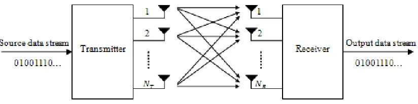
Figure 1.1 shows the block diagram of a MIMO wireless system that has N_T transmit and N_R receive antennas. The source data stream is fed to the transmitter block, after a series of data processing including data compression and channel coding, the data stream is encoded and divided into separate symbol streams, which can be independent, partially redundant or fully redundant. Each symbol stream is then sent to one of the transmit antennas and transmitted over the wireless channel after frequency up conversion and amplification.

At the receiver, the signal received by each receive antenna is a linear combination of the signals transmitted from all N_T transmit antennas plus noise. After amplification and frequency down conversion, the decoder combines the received signals from all N_R

receive antennas into one data stream and detects the transmitted data streams.

(19)

4

1.2 Diversity Techniques

Diversity techniques are widely applied in wireless MIMO systems to combat deep fading in the path. By increasing the diversity order of the transmitted signals, same information will be carried by signals through multiple independent fading channels, and thus the probability that all signals will encounter the same deep fading will be minimized [24]. Three of the conventional diversity techniques are time diversity, frequency diversity and space diversity.

Time diversity techniques involve transmitting signals with the same information in diverse time slots [24]. Since the transmitted signals are independent with each other, the received signals in each time slot will experience independent fading. An example of time diversity techniques in practical wireless systems is the forward error control (FEC) coding in conjunction with time interleaving.

In frequency diversity techniques, signals carrying the same information are transmitted over different carrier frequencies [32]. To guarantee that different frequencies experience different fading, the carrier frequencies must be separated with each other by more than one coherent bandwidth of the channel. The RAKE receiver is generally considered as on form of frequency diversity.

(20)

5

1.3 Space-Time Coding Background

As discussed in previous sections, the MIMO system cooperated with various diversity techniques can provide the wireless communication system higher resistance to multipath fading effect. Another fact is that the capacity of the MIMO channel increases linearly with min

(

NT,NR

)

. In other words, the capacity of the wireless system can be improved

by increasing the spatial diversity order without extra power and bandwidth consumption. This leads to the development of space-time and space-frequency codes (STC & SFC).

By applying a well designed STC or SFC to the MIMO system, the spatial diversity order can be maximized and so does the system capacity. STC is accomplished in space and time domain, while SFC is done in space and frequency domain. In this thesis, we will concentrate on the study of STC.

In 1996, Gerard Foschini proposed the laboratories layered space-time (BLAST) architecture at Lucent Technologies' Bell Laboratories. This is the first STC architecture in the world that exploits the concept of spatial multiplexing and provides high data rate transmission. The problem of this technique, however, is that it only provides some diversity gain at the receiver and does not provide any transmit diversity.

(21)

6

1.4 Research Objective and Contributions

As stated in section 1.3, STBC has proved to be an effective technique to combat multipath fading effect and achieve transmit diversity, due to its high diversity order and low decoding complexity. So far, most research on STBC has assumed that cooperative transmit antennas are perfectly synchronized and the receiver has full knowledge of the channel state information (CSI). Such assumptions, unfortunately, is difficult or even impossible to be satisfied in many practical systems: imperfect synchronization because of the drifting of parameters of electronic components and the lack of common clock oscillator in low-cost cooperative systems, and partial knowledge of CSI because of the channel estimation can never be perfect and fading factors derived from pilot symbols cannot represent the channels for data symbols in fast fading environment [32].

This research is motivated by problems listed above, and the goal of this thesis is to propose a simple and novel receiving scheme for the basic Alamouti’s two-branch STBC system when both perfect channel estimation and synchronization are unavailable.

The main contributions of this thesis are:

z Evaluated the performance of Alamouti’s 2-branch STBC system under imperfect channel estimation and synchronization.

z Established system models for imperfect channel estimation and synchronization.

(22)

7

1.5 Organization of the Thesis

The organization of this thesis is as follows:

In Chapter 2, STC system is discussed in detail with emphasis on the two-branch STBC scheme. A comparison of STBC and maximal-ratio receiver combining (MRRC) is also presented in this chapter.

Chapter 3 presents performance analysis for STBC under imperfect synchronization and channel estimation, and introduces existing techniques addressing STBC under imperfect conditions with emphasis on four state of the art techniques, including the block-based equalization (BE-STBC), the parallel interference cancellation, the antenna selection technique (AS) and the power allocated quasi-orthogonal STBC (PQO-STBC).

In Chapter 4, the minimum mean square error (MMSE) estimator is introduced systematically with emphasis on the linear minimum mean square error (L-MMSE) estimator.

Chapter 5 develops the proposed receiver. System models of imperfect channel estimation and rough synchronization are established first, followed by the deduction of proposed receiver based on these models.

Chapter 6 presents the simulation results, which include the BER performance of the proposed receiver and conventional designs for comparison.

(23)

8

Chapter 2 Space-Time Codes

STC is a coding technique used in Wireless communication systems to combat channel fading effect. Using multiple transmit and receive antennas the technique provides high diversity order and spatial multiplexing gain. Appling STC to a MIMO system maximizes power and bandwidth efficiency, as well as the system capacity. There exist two major classes of STC, the space-time block codes (STBC) and space-time trellis codes (STTC). Both satisfy the Rank Criterion and achieve full diversity order. In this chapter, structures of both STC classes are described with emphasis on Alamouti’s two-branch STBC.

2.1 Space-Time Trellis Codes

(24)

9

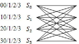
symbol. Two adjacent encoded symbols are then transmitted simultaneously by two transmit antennas. Table 2.1 shows an example of this transmission sequence. The information symbols after 4-PSK modulation shown in Figure 2.2 is 1,3,1,2,0,1,0,0,3,…, then after the initial state, the second state is S₁ because the first symbol is 1. In the first time slot, two symbols 0 and 1 will be transmitted by antenna 0 and 1, respectively. The encoding process keeps on going like this until all of the information symbols are encoded. The bandwidth efficiency of this scheme is 2 bits/sec/Hz.

Figure 2.1: Four-State Space-Time Trellis Diagram.

(25)

10

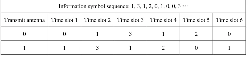
Information symbol sequence: 1, 3, 1, 2, 0, 1, 0, 0, 3 …

Transmit antenna Time slot 1 Time slot 2 Time slot 3 Time slot 4 Time slot 5 Time slot 6

0 0 1 3 1 2 0

1 1 3 1 2 0 1

Table 2.1: Transmission Sequence of Four-State STTC.

The major challenge of implementing STTC in practice is that the decoding complexity of STTC increases exponentially with transmission rate and number of transmit antennas [29]. In this scenario, space-time block coding is more appropriate to use due to its low decoding complexity.

2.2 Space-Time Block Codes

(26)

11

2.2.1 Alamouti’s Scheme

In Alamouti’s STBC model, the encoder encodes a block of two modulated symbols s₀

and s₁ at a time both in space and time domain, which is why it is called space-time block codes. The code matrix for two-branch STBC is specified as

* 0 1 * 1 0

s s

⎡ − ⎤

= ⎢ ⎥

⎣ ⎦

S . (2.1)

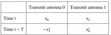
Row 1 and 2 represent transmit antenna 0 and 1, respectively. Column 1 and 2 represent time slot 1 and 2, respectively. The encoding and transmission sequence is shown in Table 2.2. In time slot 1, antenna 0 transmits s₀ and antenna 1 transmits s₁. In time slot 2, antenna 0 transmits *

1

s

− and antenna 1 transmits * 0

s , where

[ ]

⋅* denotes “complex conjugate”. Since two symbols are transmitted in two symbol time slots, Alamouti’s two-branch STBC is the first and only STBC scheme that achieves full data rate.

Transmit antenna 0 Transmit antenna 1

Time t ݏ଴ ݏଵ

Time t + T െݏଵכ ݏ଴כ

Table 2.2: Encoding and Transmission Sequence of Alamouti’s STBC.

(27)

12

through a quasi-static flat fading channel. Since each transmit antenna goes through a different path to reach the receiver, the channel fading coefficients vector may be represented as

[

0, 1

]

T

h h =

h . (2.2)

where

[ ]

⋅T denotes “transpose” and jm

m m

h =α e θ , m=1, 2, is the channel fading gain from transmit antenna m to the receiver. These fading factors are assumed to be independent and have Rayleigh distributed amplitudes. At the receiver, if we assume that both transmitters are perfectly synchronized with the receiver, the received signals may be represented as

*

0 0 1 1 0

0 0

0 1

* *

*

0 1 1 0 1

1 1

1 0

T

T s s h n h s h s n

h s h s n

h n s s + + ⎡ − ⎤ ⎡ ⎤ ⎡ ⎤ ⎡ ⎤ = + =_⎢ _⎥ _{⎢ ⎥ ⎢ ⎥}+ =_⎢ _⎥ − + + ⎣ ⎦ ⎣ ⎦ ⎣ ⎦ ⎣ ⎦

r S h n , (2.3)

where n is the additive white Gaussian noise vector which is composed of CN

(

0,σ_n2

)

distributed noise samples.

The decoder for Alamouti’s two-branch STBC consists of three major parts including channel estimator, linear combiner and maximum likelihood (ML) detector. If the receiver has full knowledge of the CSI, then the channel estimations derived from channel estimator are the same as the real channel factors. The linear combiner is an estimator of the transmitted symbols. It combines the received signals and the channel fading factors with a simple linear combination rule. The combination rule is given by

* *

0 0 0 1 1

* *

1 1 0 0 1

ˆ ˆ

ˆ

s h r h r

⎡ + ⎤

⎡ ⎤

=_{⎢ ⎥} _{= ⎢} _⎥ −

⎣ ⎦ ⎣ ⎦

(28)

13

Substitute (2.3) into (2.4), the estimations of transmitted symbols would be

(

)

(

)

2 2 * *

* *

0 1 0 0 0 1 1 0 0 0 1 1

* * ₂ ₂ _* _*

1 1 0 0 1 ₀ ₁ ₁ ₁ ₀ _{0 1}

ˆ ˆ

ˆ

s h n h n

s h r h r

s h r h r _s _{h n} _{h n}

α α

⎡ + + + ⎤

⎡ + ⎤

⎡ ⎤ _⎢ _⎥

=_{⎢ ⎥}=_⎢ _⎥=

− ⎢ ₊ ₊ ₋ ⎥

⎣ ⎦ ⎣ _{⎦ ⎣} _⎦

s . (2.5)

The estimated symbols then pass to the ML detector where hard decisions are made. The hard decision criteria used in the ML detector is the squared Euclidean distance (SED). The SED between x and y is defined as

( ) (

)

(

)

2 * *

,

d x y = x−y x −y . (2.6)

The decision rule:

choose s_i if and only if

(

₂ ₂

)

2 ₂

(

)

(

₂ ₂

)

2 ₂

(

)

0 1 1 si d s sˆ0, i 0 1 1 sk d s sˆ0, k

α +α − + ≤ α +α − + , ∀ ≠i k (2.7)

is used to decode s₀ and

choose s_i if and only if

(

₂ ₂

)

2 ₂

(

)

(

₂ ₂

)

2 ₂

(

)

0 1 1 si d s sˆ1, i 0 1 1 sk d s sˆ1, k

α +α − + ≤ α +α − + , ∀ ≠i k (2.8)

is used to decode s₁.

(29)

14

simple since symbols s₀ and s₁ can be decoded individually. Figure 2.3 demonstrates the block diagram of Alamouti’s two-branch STBC model.

The Alamouti’s STBC can also accommodate multiple receive antennas. A generalized STBC model with an arbitrary number of transmit and receive antennas is given in next section. The discussion is brief and introductory since it is not the subject of this thesis. To readers who are interested in STBC with multiple transmit and receive antennas, investigations and discussions can be found in detail in [32] and the references therein.

Figure 2.3: Block Diagram of Alamouti’s STBC.

2.2.2 Generalization of STBC System Model

(30)

15

design, extended STBC schemes can achieve partial diversity order and low decoding complexity [32].

A generalized STBC system is considered with N_T transmit antennas and N_R receive antennas. The encoder encodes a block of p information symbols at a time and generates q encoded symbols for each transmit antenna. The system achieves full data rate for p = q and partial rate for p < q. Thus, at an arbitrary symbol time slot t, the symbol transmitted by each transmit antenna may be represented as s t_i

( )

, i=1, 2,_LN_T. An example of extended STBC schemes is the partial rate STBC with 3 transmitting antennas. The code matrix for this scheme is given by

* *

0 1 2

* *

3 1 0 2

* *

2 0 1

0 0 0

s s s

⎡ − ⎤

⎢ ⎥

=_⎢ − _⎥

⎢ ₋ ⎥

⎣ ⎦

S .

The rows represent the symbols transmitted by each antenna. The columns represent different time slots. In this example, p = 3 and q = 4. The data rate is therefore 3/4.

Assume that the channel between each transmit antenna and receive antenna is quasi-static and flat, and time-invariant in one data frame. The channel fading coefficients matrix may be represented as

0,0 0,

,0 ,

R

T T R

N

N N N

h h

⎡ ⎤

⎢ ⎥

= ⎢ ⎥

⎢ ⎥

⎣ ⎦

H

L

M O M

L

, (2.9)

(31)

16

slot t is a linear combination of signals transmitted from all transmit antennas and may be represented as

( )

,

( )

,

1

T

N

j i j i i j

i

r t h s t n

=

∑

+ , (2.10)

where n_{i j}_, is a complex random variable represents the receiver noise and interference in each channel. For additive white Gaussian noise (AWGN) channel, n_{i j}_, has the distribution of

(

)

,

2

0,

i j n

σ

CN .

2.3 Simulation Results for STBC

In this section, we present error performance simulation for Alamouti’s in Rayleigh fading channel. For all simulations, information symbols are BPSK modulated and un-coded by any other channel encoders.

(32)

17

(33)

18

Chapter 3

Performance of STBC with Imperfect

Channel Estimation and Synchronization

In this chapter, we study the performance of STBC when both perfect knowledge of CSI and synchronization are unavailable. This chapter is organized as follows. In Section 3.1, we build the noisy CSI model and perform system analysis. Simulations are also given at the end of this section. Approximate models for received STBC signals combined with inter-symbol interference (ISI) have been built in Section 3.2. The impact of imperfect synchronization has been described and simulated in succession. In Section 3.3, we give background introductions to some state of the art techniques addressing STBC under noisy CSI and imperfect synchronization.

3.1 Effect of Imperfect Channel Estimation

(34)

19

transmitter [1]. In practical MIMO systems, these coefficients must be estimated, which are usually not accurate, thereby leading to the performance degradation [9]. On the other hand, there is an elementary trade-off between the channel estimation accuracy and system capacity. Since estimation of channel fading factors requires overhead training data sequences, or so called pilot symbols. Increasing the number of pilot symbols may improve the accuracy of the channel estimation [16]. However, this will cause the sacrifice in data rate, and thus leading to the system capacity degradation. It is also shown in [12] that as the number of transmit and receive antennas increases the system becomes more dependent on the channel estimation accuracy.

Although perfect channel fading coefficients are impossible to get in practice, the receiver might have partial knowledge of CSI, with this partial knowledge, variance of the channel estimation error can be derived. It has been proved in [29] that the system performance can be improved by introducing this information into the decision rule. In this section, we consider modeling of estimation error of the CSI and investigate BER performance for Alamouti’s STBC with both perfect and estimated channel state information.

3.1.1 System Model of STBC with Imperfect Channel Estimation

(35)

20 ˆ

h= +h e, (3.1)

where e is the channel estimation error. Without loss of generality, we assume that e is a complex Gaussian random variable with zero mean and variance of 2

e

σ . We also assume

that e is independent of h. Hence the variance of estimation of channel fading factor 2 ˆ

h

σ

can be written as

2 ˆ

2 2

h

h e

σ =σ +σ , (3.2)

where 2

h

σ is the variance of the real channel fading factor. The correlation between h

and ˆh can be expressed by 2

e σ as

ˆ ₂

1 1

h h

e

σ

= +

C . (3.3)

Since this model of channel estimation is general and widely accepted, we use it in our work. To evaluate the effect of imperfect channel estimation, let us first examine the pair-wise error probability based on this model [29]. Consider a basic model of STBC with N transmitting and M receiving antennas. The information symbol s i

( )

at symbol time slot i is encoded by the STBC encoder as c i c i₀

( ) ( )

, ₁ _Lc_N₋₁

( )

i . Each code symbol is transmitted simultaneously from a different transmit antenna. Assuming ideal time and frequency synchronization, the base-band signal received by the receive antenna

0,1 1

(36)

21

( )

1

( ) ( )

( )

0 2

N

k s jk j k

j

r i E h i c i n i

−

=

∑

+ , (3.4)

where 2Es is the average energy of the base-band signal. The coefficient hjk

( )

i is the

channel fading factor between transmit antenna j and receive antenna k at time slot i. The additive noise n i_k

( )

is an independent sample of the base-band white Gaussian process with CN

(

0,σ_n2

)

distribution. Let

( )

0

( ) ( )

, 1 1

( )

T N

i = ⎡⎣c i c i c − i ⎤⎦

c _L ,

( )

0

( ) ( )

, 1 1

( )

T j i = ⎣⎡hj i hj i hjM− i ⎤⎦

h _L ,

( )

1

( ) ( )

, 2 1

( )

T N

i = ⎡_⎣ i i ₋ i ⎤_⎦

H h h _Lh ,

( )

0

( ) ( )

, 1 1

( )

T M

i = ⎡_⎣n i n i n ₋ i ⎤_⎦

n _L ,

( )

0

( ) ( )

, 1 1

( )

T M

i = ⎡_⎣r i r i r ₋ i ⎤_⎦

r _L .

The received signals at time slot i by all receive antennas can therefore be written in a matrix form as

( )

i = 2E_s

( ) ( )

i i +

( )

i

r H c n , (3.5)

(37)

22

0,0 0, 1

1,0 1, 1

L

N N L

p p p p − − − − ⎡ ⎤ ⎢ ⎥ = ⎢ ⎥ ⎢ ⎥ ⎣ ⎦ P L

M O M

L

, (3.6)

where rows represent pilot symbols transmitted from different antennas. Columns represent different index in different pilot symbol sequences. In our study, pilot symbol sequences for all transmit antennas are orthogonal to each other.

Let the received pilot symbols and noise be given by

0,0 0, 1

1,0 1, 1

p p L

p N p N L

r r r r − − − − ⎡ ⎤ ⎢ ⎥ = ⎢ ⎥ ⎢ ⎥ ⎣ ⎦ P R L

M O M

L

; (3.7)

0,0 0, 1

1,0 1, 1

p p L

p N p N L

n n n n − − − − ⎡ ⎤ ⎢ ⎥ = ⎢ ⎥ ⎢ ⎥ ⎣ ⎦ P n L

M O M

L

. (3.8)

Using (3.6), (3.7) and (3.8), (3.5) can be rewritten as

2E_s

= +

P P

R HP n . (3.9)

The minimum mean square estimate of H can be obtained from (3.9) as

(

)

1

2 ˆ 1 2 1 / 2 H H s H s E E − = = P P

R P PP

R P P H

(38)

23 Combining (3.9) and (3.10) , we have

2 1 / 2 ˆ H s E + = = + P

H n P P

H H

e (3.11)

where e is the estimation error matrix given by

2 1 / 2 H s E = _P

e n P P (3.12)

Assuming a N ×L code matrix

0,0 0, 1

1,0 1, 1

L

N N L

c c c c − − − − ⎡ ⎤ ⎢ ⎥ = ⎢ ⎥ ⎢ ⎥ ⎣ ⎦ C L

M O M

L

(3.13)

is transmitted. The probability that the ML detector decides in favor of other code matrix

0,0 0, 1

1,0 1, 1

L

N N L

c c c c − − − − ⎡ ⎤ ⎢ ⎥ = ⎢ ⎥ ⎢ ⎥ ⎣ ⎦ C

% L %

% _M _O _M

% L %

(3.14)

based on the imperfect estimation of the channel fading gain is given by [29]

(

)

( )

(

)

2 2 ˆ ₂ ˆ 0 ˆ

| exp ,

4 4 1

s

s E

P d

N N E

⎛ ⎞ ⎜ ⎟ → ≤ _⎜− _⎟ + − ⎜ ⎟ ⎝ ⎠ HH HH

C C H% C C C%

C

, (3.15)

(39)

24

( )

1 1 1

(

)

(

)

2

2 1 1

ˆ ,

0 0 0

ˆ _ˆ

, / 2

M L N

n n

m n h l l

m l n

d h σ

− − −

+ +

= = =

=

∑ ∑ ∑

−

C C% c c . (3.16)

Intuitively, for Alamouti’s STBC, the effect of noisy CSI can be best shown by combining the received signals and estimated channel fading factors with the linear combiner described in (2.5). Assuming the CSI is perfectly known to the receiver, which means hˆ₀ =h₀ and hˆ₁ =h₁, the outputs of the linear combiner are given by

(

2 2

)

* * * *

0 0 0 1 1 0 1 0 0 0 1 1

ˆ h r h r h h s h n h n;

s = + = + + + (3.17)

(

2 2

)

* * * *

1 1 0 0 1 0 1 1 1 0 0 1

ˆ h r h r h h s h

s = − = + + n −h n . (3.18)

For imperfect channel estimation, we use the model in (3.11) and derive following combined signals:

(

)

(

) (

)

* *

0 0 0 1 1

2 2 * * * * * * * *

0 1 0 0 0 1 1 0 0 1 1 0 1 0 0 1 1 0 0 1 1

ˆ ˆ

ˆ r r

h h s e h e h s e h e h s h n h n e n e n

s =h +h

+ +

= + + − + + + + ; (3.19)

(

)

(

) (

)

* *

1 1 0 0 1

2 2 * * * * * * * *

0 1 1 1 0 0 1 0 1 1 0 0 1 0 0 1 1 1 0 0 1

ˆ ˆ

ˆ r r

h h s e h e h s e h e h s h n h n e n e n

s =h −h

+ +

(40)

25

3.1.2 Simulations

In this section, we analyze the performance of a cooperative STBC system with two relay nodes and one receiver under imperfect channel estimation. BPSK modulation is applied and the signal to noise ratio (SNR) is defined as 2 2

( )

SNR=σ σs n dB . We assume that the signals transmitted from two transmit antennas are perfectly synchronized with each other both in time and frequency. We also assume that the channel is quasi-static and Rayleigh fading. The bit error rates (BER’s) of the conventional STBC receiver with imperfect channel estimation under different values of 2

e

σ are shown in Figure 3.1. The performance of perfect channel estimation is also given for comparisons.

(41)

26

3.2 Effect of Imperfect Synchronization

So far, we have assumed that the transmitters are perfectly synchronized in the STBC system, which means signals from different transmit antennas arrive at the receiver at the same time. However, in many practical STBC systems, this assumption is difficult or even impossible to achieve.

One of the many popular applications of STBC in practice is to combine STBC with a distributed wireless system, such as an ad-hoc or a wireless sensor network [10]. This kind of application is commonly known as cooperative transmission since the distributed transmitters in the network will cooperate with each other and apply STBC to increase the system capacity. In such systems, common local clock oscillator among different transmitters is always unavailable [17]. Furthermore, due to the restriction of the cost and size of the transmitters, the parameters of electronic components may also be drifting. Another fact is that the delay synchronization with respect to two or more receive antennas simultaneously is impossible. Therefore, at the receiver, there will be small time misalignments among the signals from different transmit antennas [17].

The synchronization problem in cooperative transmission has been investigated in [17-20, 34, 37-38]. Imperfect synchronization in time will introduce inter-symbol interference (ISI). For a STBC coded system, this interference will jeopardize the required orthogonal structure and thus makes the conventional STBC linear decoding method fail.

(42)

27

3.2.1 System Model of STBC with Imperfect Synchronization

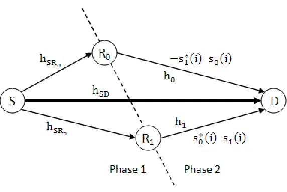
We consider a 4-node cooperative STBC system depicted in Figure 3.2.

Figure 3.2: Cooperative STBC Model with 2 Relay Nodes.

In Phase I, the source node S broadcast its information to potential relay node (R0 and R1)

and the destination node D. The coefficient h_SD denotes the channel fading gain between S and D, while

n

SR

h denotes the channel fading gain between S and relayR_n.

In phase II, S stops transmission, R0 and R1 cooperate with each other and encode the

(43)

28

There are two different transmission schemes for each relay: one is amplify-and-forward (A&F), another is decode-and-forward (D&F) [32]. In the A&F scheme, the relays just amplify the received signals and send them to the destination after STBC processing, while in the D&F scheme, each relay detects the source information data first, and only the relays that can successfully detect the source information will be cooperate with each other and perform STBC encoding. In our case, we use the D&F scheme and assume that all relays can detect the source information successfully, and they will be both enrolled in Phase II transmission.

Denoting the ith modulated symbol generated by the source as

( )

( ) (

)

j ct

s i =Ab i p t−iT e ω , (3.21)

where b i

( )

is the complex symbol transmitted at symbol interval ⎡_⎣iT i,

(

+1

)

T⎤_⎦,

(

)

p t iT− is the base-band pulse shaping filter associated with the ith symbol. The positive scalar A denotes carrier amplitude and ω_c is the carrier frequency. After a packet of two modulated symbols is received and detected by R0 and R1, the two relays

will apply STBC encoding to the symbol packet and send the encoded symbols to the destination. The encoded STBC symbols can be expressed by the matrix:

( )

*

0 1

*

1 0

s i s i

⎡ − ⎤

= ⎢ ⎥

⎣ ⎦

S . (3.22)

(44)

29

( )

( ) (

)

( c n)

_{( )}

p j t

n n n n n

s i =α Ab i p t iT− −τ e ω θ− +n i , (3.23) where α_n is the multipath fading gain of the channel between relay n and the destination.

Term

( )

p

n

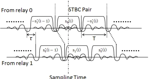
n i is the pass-band noise, while τ_n and θ_n denote time delay and phase shift, respectively. The relative delay between R0 and R1 is therefore given byτ τ τ= −1 0.

The received signals at the data collector are linear combinations of s_n

( )

i . When the time delay and frequency offset between R0 and D are different with those between R1

and D, imperfect synchronization problem occurs. Figure 3.3 (a—c) shows the effect of time errors on sampling process at the receiver.

(45)

30

(b) τ ≤0.5T Imperfect Synchronization

(c) τ >0.5T Imperfect Synchronization

Figure 3.3: Impact of Imperfect Synchronization between 2 Relay Nodes.

(46)

31

different relays have different τ_n and θ_n [23], we demodulate the signal with local carrier _e−j tωc _{and perform sampling at time instances}

0

s

iT +t and

(

i+1

)

T_s +t₀ (for arbitrary t₀). Assuming the channel is quasi-static, the base-band samples therefore can be given by

( )

( ) (

)

(

( )

)

(

( )

)

( )

(

)

(

( )

)

( )

1

' *

0 0 0 1

0

*

1 0 0

[

]

n j

n n n

n k i k

k i k

r i A b i p t e ISI s k ISI s k

ISI s k ISI s k n i θ α τ − +∞ = ≠ =−∞ +∞ ≠ =−∞ = − + + − + + +

∑

(3.24)

( )

( ) (

)

( ) (

)

(

( )

)

( )

(

)

(

( )

)

(

( )

)

( )

0 1 '

1 0 1 0 1 1 0 0 0 0

* *

1 1 0 1

[

] ,

j j

k

k i k k i

r i A b i p t e b i p t e ISI s k

ISI s k ISI s k ISI s k n i

θ θ α τ α τ +∞ =−∞ +∞ ≠ =−∞ ≠ = − − + − + + − + + +

∑

(3.25)

where r_m'

( )

i represents the received signal at symbol time slot

(

i+m T

)

_s and n i_n

( )

is the base-band noise. We use the prime variables to indicate that the received signals contain ISI. Equations (3.24) and (3.25) can be further simplified as

( )

'

0 0 0 1 1 00 01 0

r i =h s i +h s i +I +I +n i ; (3.26)

( )

' * *

1 0 1 1 0 10 11 1

r i = −h s i +h s i +I +I +n i , (3.27)

where jn

n n

h =α e θ denotes the channel between the relay n and the destination D. I_mn

represents the ISI experienced by '

( )

m

(47)

32

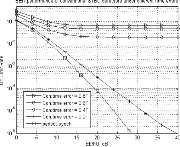
3.2.2 Simulations

In this section, we analyze the performance of a cooperative STBC system with two relay nodes and one receiver under imperfect synchronization. BPSK modulation is applied and the signal to noise ratio (SNR) is defined as 2 2

( )

SNR=σ σs n dB . We assume that the receiver has perfect knowledge of the carrier frequency of each transmitter, as well as the fading coefficient of each channel. We also assume that the channel is quasi-static and Rayleigh fading. The bit error rates (BER’s) of the conventional STBC receiver with imperfect synchronization under different values of τ are shown in Figure 3.4. The performance of conventional STBC under perfect synchronization is also given in the simulation for comparison.

(48)

33

3.3 Previous Works

A summary of the existing techniques addressing STBC under imperfect channel estimation is as follows. The partial knowledge of CSI was discussed and a modified decision rule was proposed by Tarokh in [29]. The effect of imperfect channel estimation on STBC is analyzed in [9], [12], and [15]. Power-allocated quasi-orthogonal STBC is studied in [13]. Antenna selection technique is discussed in [21]. Analytical evaluation of the diversity combining technique under imperfect channel estimation is studied in [36]. All of above works assume that the transmitters and receivers are synchronized both in timing and frequency.

(49)

34

Chapter 4 Linear MMSE Estimator

Estimation theory, which can be found at the heart of many modern electronic signal processing systems, is a branch of statistic that deals with estimating the values of a group of parameters based on observed or measured signals [16]. Based on the type of parameters of interest, approaches to statistic estimation can be divided into two major categories: the estimation of deterministic but unknown constants and the estimation of random variables. We consider the latter case only since all signals in our study are random variables. In order to estimate the parameters of interest, it is first necessary to determine a system model in which the parameters, as well as the points of uncertainty and noise, can be described. After deciding upon a model, an estimator needs to be developed or applied if an existing estimator is valid for the model.

(50)

35

4.1 Minimum Mean Square Error Estimator

In statistics, the mean square error (MSE) of an estimator is one of many ways to quantify the difference between an estimator and the true value of the quantity been estimated [16]. MSE measures the average of the square of the error. The error occurs because of the randomness or because the estimator dose not account for information that could produce a more accurate estimate. The MSE of an estimator sˆ with respect to the estimated parameter s is defined as [16]

(

)

2

ˆ ˆ

( ) [ ]

MSE s =E s s− , (4.1)

where E

[ ]

⋅ is the expectation operator. Since s is a random variable, the expectation operator is with respect to the joint pdf p

( )

r,s , where r is the sequence of observed or

measured signals. Thus (4.1) can be rewritten as

(

) ( )

2

ˆ ˆ

( ) ,

MSE s =

∫∫

s−s p r s d dsr (4.2)

Using Bayes’ theorem, p

( )

r,s can be rewritten as

( )

,

( ) ( )

|

p r s = p s r p r . (4.3)

Substituting (4.3) into (4.2), we have

(

) ( )

2

( )

ˆ ˆ

( ) |

MSE s =

∫ ∫

⎡_⎣ s s− p s r ds p⎤_⎦ r rd . (4.4)

(51)

36

( )

(

)

(

) ( )

( )

2 2 ˆ ˆ

arg min arg min

ˆ

arg min |

MSE s E s s

s s p s ds p d

⎡ ⎤

= _⎣ − _⎦

⎡ ⎤

=

∫ ∫

_⎣ − r _⎦ r r

To minimize (4.4), we fix r and derive the partial derivative of the integral in brackets with respect to s as

(

) ( )

(

) ( )

(

) ( )

( )

2 2 ˆ | ˆ | ˆ 2 | ˆ

2 | 2 |

s s

s s p s ds s s p s ds

s s p s ds

sp s ds s p s ds

∂ ₋ ₌ ∂ ₋ ∂ ∂ = − − = − +

∫

r r r

r r (4.5)

Set (4.5) to zero results in

( )

[ ]

ˆ |

| s sp s ds

E s = =

∫

r

r (4.6)

Therefore, (4.6) is the MMSE estimator that minimizes E⎡_⎣

(

s−sˆ

)

2⎤_⎦.

(52)

37

4.2 Linear MMSE Estimator

Since the evaluation of mean requires integration, the estimator shown in (4.6) cannot be used in practice. For practical MMSE estimators, we need to be able to express them in a closed form. One of many methods to determine a closed form for a MMSE estimator is to seek the technique minimizing MSE within a particular class, such as the class of linear estimators. The linear MMSE (L-MMSE) estimator is the estimator achieving minimum MSE among all estimators of the form a X +b [16]. In this section, we concentrate on the class of linear estimators and derive the general closed form for the linear L-MMSE estimator.

We begin our discussion by assuming a parameter s is to be estimated based on single received signal r. The parameter s is models as the realization of a random variable. Later on, the solution is extended to multiple received signals. A linear estimation sˆ of a

transmitted symbol s using the received signal r is

( )

ˆ

s r =ar+b, (4.7)

where sˆ and r are random variables. Choosing the weighting coefficients a and b to minimize the Mean Square Error (MSE) based on a measurement of r:

2

ˆ ˆ

( ) [( ) | ]

MSE s =E s−s r . (4.8)

(53)

38

2

[( ) ] 2 [( ) | ]

2 [ | ] 2 [ | ] 2 [ ] 2 [ ] 2 [ ] 2

E s ar b r E s ar b r b

E s r E ar r E b

E s aE r b

∂ ₋ ₋ _{= −} ₋ ₋

∂

= − + +

= − + + (4.9)

Please be noted that for continuous random signals, acknowledgement of single deterministic measurement will not change the mean of the signals. This theorem can be proved by the following equation:

[

|

]

r r R|

( )

[ ]

E r r R αf α αd E r

+∞ = −∞

= =

_∫

= ,

where R is a single deterministic measurement of r.

Setting (4.9) to zero produces

[ ]

b=E s −aE r . (4.10)

Substituting (4.10) into (4.8), the MSE can be rewritten as

2 2

2 2 2

ˆ

( ) [ [ ] [ ] ] [( [ ]) ( [ ]) ]

[ [ ] ] 2 [ [ ] [ ]] [ [ ] ] MSE s E s ar E s aE r

E s E s a r E r

E s E s aE s E s r E r a E r E r

= − − +

= − − −

= − − − − + − . (4.11)

If the means of s and r are zero, then

( )

2

ˆ _ss 2 _sr _rr

MSE s =C − aC +a C , (4.12)

(54)

39

( )

ˆ

2 rr 2 sr MSE s

a a

∂

= −

∂ C C ,

which when set to zero results in

1

rr sr

a=C C− . (4.13)

Substitute (4.10) and (4.13) into (4.7) yields

1 1

1

ˆ( )

[ ] [ ]

[ ] ( [ ])

rr sr rr sr

rr sr

s r ar b

r E s E r

E s r E r

− −

−

= +

= + −

C C C C

C C (4.14)

This is the L-MMSE estimator for single random variable based on single received signal. If the means for s and r are zero, then

( )

1

ˆ _rr _sr

s r =C C− r. (4.15)

The minimum MSE is then given by substituting (4.13) into (4.12):

1 2

2 1 2 2 2

2 1

ˆ

( ) [( ) ]

[ ] [2 ] [ ]

rr sr

rr sr rr sr

ss sr rr

MSE s E s r

E s E s r E r

− − − − = − = − + = − C C

C C C C

C C C (4.16)

Now we extend the solution to multiple received signals. The L-MMSE estimator for a random variable based on multiple received signals does not entail anything new but only a need of vector calculations.

(55)

40

( )

ˆ T

s r =a r+b,

wherea=

[

a a₀, ₁…aN−₁

]

T. N is the number of received signals. By applying the same

procedure shown above, the solution of L-MMSE estimator for a random variable based on multiple received signals can be derived as

-1

s

= _rr _r

a C C ,

[ ]

T

[ ]

b=E s −a E r ,

( )

[ ]

1

(

[ ]

)

ˆ _s

s r =E s +C C_r _rr− r−E r ,

where Crr is the N ×N covariance matrix of r, and Csr is the 1×N cross-covariance

vector having the property that T sr = rs

C C .

If the means for s and all elements in r are zero, then

( )

1

ˆ _s

(56)

41

Chapter 5 Proposed Receiver for STBC with

Imperfect Channel Estimation and

Synchronization

(57)

42

This chapter is organized as follows. Section 5.1 gives background information of this chapter and the previous works in this area. Section 5.2 describes system models and assumptions used in this chapter. The derivation of the proposed receiver is given in Section 5.3. In Section 5.4 we compare the proposed receiver with conventional STBC detector, and investigate the relationship between the L-MMSE estimator and Alamouti’s conventional linear combiner. Section 5.5 studies some advantages and disadvantages of the proposed receiver and concludes the chapter.

5.1 Background and Previous Works

Diversity techniques have been widely utilized in wireless communication systems to improve the system capacity and to combat channel fading [10]. Space-Time block coding (STBC) combines space and time diversity techniques and applies two transmit antennas and one receive antenna to increase the system resistance to multipath fading effect [32]. As stated earlier in Chapter 2, STBC is attractive to researchers because it provides high diversity order with low decoding complexity. Such outstanding features, however, is only achievable under perfect synchronization and channel estimation. In most of practical STBC applications such as the cooperative transmission, the multiple transmitters can never be precisely synchronized with each other. In addition, the receiver never has the perfect knowledge of CSI, since the channel fading factors are random variables. In such cases, the conventional receiver is no longer able to remove the cross-terms due to the mismatch in time and CSI, and thus the entire STBC system fails.

(58)

43

in papers such as [15] and references therein. Beside of existing works addressing STBC for the joint problems, more works have been for other coded systems such as Turbo codes. For example, joint synchronization and channel estimation problem has been addressed by Sun and Valenti in [27] for Turbo codes; the utilizing of channel estimation error variance in the decision rule appears in Frenger’s paper also for Turbo coded systems [7],[8]. Similar approaches can be taken here with different system models.

5.2 System Models and Assumptions

(59)

44

demodulator and source decoder to recover the source information [32].

Figure 5.1: Block Diagram of Alamouti’s STBC System.

As stated in Chapter 2, the code matrix for Alamouti’s two-branch STBC is specified as

* 0 1 * 1 0

s s

⎡ − ⎤

= ⎢ ⎥

⎣ ⎦

S .

We assume that the wireless channel is flat fading and quasi-static, so that the channel fading factors are constant over a symbol frame and vary from one frame to another. Since each transmit antenna goes through a different path to reach the receiver, the channel fading coefficients vector may be represented as

[

0, 1

]

T

h h =

h .

(60)

45

Gaussian random variables with Rayleigh distributed amplitudes. The received signals with perfect synchronization may be represented as

*

0 0 1 1 0

0 0

0 1

* *

*

0 1 1 0 1

1 1

1 0

T

T s s h n h s h s n

h s h s n

h n s s + + ⎡ − ⎤ ⎡ ⎤ ⎡ ⎤ ⎡ ⎤ = + =_⎢ _⎥ _{⎢ ⎥ ⎢ ⎥}+ =_⎢ _⎥ − + + ⎣ ⎦ ⎣ ⎦ ⎣ ⎦ ⎣ ⎦

r S h n . (5.1)

The linear combiner combines the received signals and the channel fading factors estimated by the channel estimator with a simple linear combination rule given by

* *

0 0 0 1 1

* *

1 1 0 0 1

ˆ ˆ

ˆ

s h r h r s h r h r s=⎡ ⎤_{⎢ ⎥}= ⎢⎡ + ⎤_⎥

−

⎣ ⎦ ⎣ ⎦. (5.2)

Substitute (5.1) into (5.2), the estimations of transmitted symbols under perfect synchronization and channel estimation would be

(

)

(

)

2 2 * *

* *

0 1 0 0 0 1 1 0 0 0 1 1

* * ₂ ₂ _* _*

1 1 0 0 1 ₀ ₁ ₁ ₁ ₀ _{0 1}

ˆ ˆ

ˆ

s h n h n

h r h r

h r h r _s _h

s

h s

s _n _n

α α α α ⎡ + + + ⎤ ⎡ + ⎤ ⎡ ⎤ _⎢ _⎥ =_{⎢ ⎥}=_⎢ _⎥= − ⎢ ₊ ₊ ₋ ⎥

⎣ ⎦ ⎣ _{⎦ ⎣} _⎦. (5.3)

Now, let us model the estimated channel fading coefficients and the estimation error caused by imperfect channel estimation. As described in Chapter 3, the estimated channel factor ˆh can be expressed by

ˆ

h= +h e. (5.4)

(61)

46

transmit antenna. Assuming ideal timing and frequency synchronization, the base-band signal received by the receive antenna can be represented as

( )

1

( ) ( ) ( )

0

2 _s _j _j

j

r i E h i c i n i

=

∑

+ , (5.5)

where 2E_s is the average energy of the base-band signal. h_j

( )

i is the channel fading factor between transmit antenna j and receive antenna at time slot i. n i

( )

is the independent base-band white Gaussian noise with CN

(

0,σn2

)

distribution. Let

( )

0

( ) ( )

, 1

T

i = ⎡_⎣c i c i ⎤_⎦

c , (5.6)

( )

0

( ) ( )

, 1

T

i = ⎡_⎣h i h i ⎤_⎦

h . (5.7)

The received signals at time slot i can thus be written as

( )

2 T

( ) ( )

( )

s

r i = E h i c i +n i . (5.8)

To estimate the channel vector h

( )

i , we transmit a sequence of L pilot symbols with each transmit antenna, which forms a 2×L pilot symbol matrix given by

0,0 0, 1 1,0 1, 1

L L

p p

− −

⎡ ⎤

= ⎢ ⎥

⎣ ⎦

P L

L , (5.9)

(62)

47

0 L1

p p

r r ₋

⎡ ⎤

= ⎣ ⎦

P

r _L , (5.10)

0 L1

p p

n n ₋

⎡ ⎤

= ⎣ ⎦

P

n _L , (5.11)

Using (5.9), (5.10) and (5.11), equation (5.8) can be rewritten as

( )

2E_s T i

= +

P P

r h P n . (5.12)

The minimum mean square estimate of h can be obtained from (5.20) as

(

)

1

2 ˆ 1 2 1 / 2 H H s H s E E − = = P P

r P PP

r P P h

(5.13)

Combining (5.12) and (5.13), we have

2 1 / 2 ˆ , H s E = + = + P

h n P P

h e h

(5.14)

where e is the estimation error matrix given by

2 1 / 2 H s E = _P

e n P P . (5.15)

Next, we model the received signal and ISI under imperfect synchronization. As shown in Chapter 3, the base-band received signals can be given by

( )

'

0 0 0 1 1 00 01 0

Space-time block coding with imperfect channel estimation and synchronization

Scholarship at UWindsor

Scholarship at UWindsor

Space-time block coding with imperfect channel estimation and

Space-time block coding with imperfect channel estimation and

synchronization

synchronization

SPACE-TIME BLOCK CODING WITH

IMPERFECT CHANNEL ESTIMATION AND SYNCHRONIZATION

AUTHOR'S DECLARATION OF ORIGINALITY

ABSTRACT

ACKNOWLEDGEMENTS

Contents

Author's Declaration of Originality ... iii

Abstract... iv

Acknowledgements ... v

List of Tables ... ix

List of Figures ... x

Abbreviations ... xii

Notations ... xiv

1. Introduction

...

1

2. Space-Time

Codes

...

8

3. Performance of STBC with Imperfect Channel Estimation and

Synchronization ... 18

4. Linear

MMSE Estimator ... 34

5. Proposed Receiver for STBC with Imperfect Channel Estimation

and Synchronization ... 41

7. Conclusions

and Future Works ... 80

Bibliography ... 83

List of Tables

List of Figures

Abbreviations

Notations

[ ]

[ ]

[ ]

( )

[ ]

{ }

{ }

(

[ ]

)

[ ]

[ ]

Chapter 1

Introduction

1.1 The MIMO System

1.2 Diversity Techniques

1.3 Space-Time Coding Background

(

)

1.4 Research Objective and Contributions

1.5 Organization of the Thesis

Chapter 2

Space-Time Codes

2.1 Space-Time Trellis Codes

2.2 Space-Time Block Codes

2.2.1 Alamouti’s Scheme

[ ]

[

]

[ ]

(

)

(

)

(

)

( ) (

)

(

)