Feasibility Analysis of Molecule Sensor for Detection and Quantification.

ABSTRACT

OCHI-OKORIE, CHIDIEBERE EBENEZER. Feasibility Analysis of Molecule Sensor for Detection and Quantification. (Under the direction of Dr. H. Troy Nagle).

The purpose of this investigation is to assess the feasibility of a molecule-sensor design for

detecting and quantifying charge-neutral compounds in particular. Neutral molecules can be

induced to translate by their exposure to a non-uniform electric field. Secondly, when a

voltage is applied across saline electrolyte, the solution responds to vibration by generating a

potential difference. The present molecule-sensor design is an attempt to combine these two

phenomena whereby electric-field induced molecular vibration is detected by the energized

electrolyte. In current experiments, the resulting sensor output deviated from theoretical

expectations. Hence, the feasibility of this sensor arrangement is still in question. Areas for

Feasibility Analysis of Molecule Sensor for Detection and Quantification

by

Chidiebere Ebenezer Ochi-Okorie

A thesis submitted to the Graduate Faculty of North Carolina State University

in partial fulfillment of the requirements for the degree of

Master of Science

Electrical Engineering

Raleigh, North Carolina

2012

APPROVED BY:

__________________ __________________

Dr. H. Troy Nagle (Chair_{) Dr. Gregory McCarty}

__________________

BIOGRAPHY

ACKNOWLEDGMENTS

TABLE OF CONTENTS

LIST OF TABLES ... v

LIST OF FIGURES ... vi

Introduction ... 1

First Phenomenon: Electric-Field Induced Neutral-Molecule Motion ... 1

Second Phenomenon: Motion-Sensitive Saline ... 6

Combining the Two Phenomena ... 10

Maximizing MMS Sensitivity... 14

Analysis Concepts ... 17

Relative Quantity of Analytes in Electrolyte Solution ... 17

Attenuation of Molecular Swing at High Frequencies ... 17

Standard Sample Approach ... 20

Nested Sweeps of Electric Field and Frequency to Discover Attenuation Ranges ... 24

Experiments ... 25

Discussion ... 29

Future Studies ... 30

REFERENCES ... 32

APPENDICES ... 33

APPENDIX A – System Design Overview ... 34

APPENDIX B – Circuit Schematics ... 35

APPENDIX C – Component Reference ... 42

APPENDIX D – Software Code ... 43

LIST OF TABLES

Table 1 Overview of Molecule-Sensor System Design ...34

Table 2 Lookup Reference for Specialized Components...42

Table 3 Routine: initialize ...43

Table 4 Routine: main ...44

Table 5 Sub-routine: freq_off() ...44

Table 6 Function: freq_out() ...45

Table 7 Function: getbd() ...45

Table 8 Function: newDArray() ...46

Table 9 Function: readPoint() ...47

Table 10 Function: readStable() ...47

Table 11 Sub-routine: saveData() ...48

Table 12 Sub-routine: set_hv_level() ...48

Table 13 Sub-routine: setFState() ...48

LIST OF FIGURES

Fig 1 E-field generator consisting of three metal “plates,” A, B, & C. ...2

Fig 2 E-field generator consisting of three metal “plates,” A, B, and C ...3

Fig 3 E-field generator as in figure 2, except with reversed polarity on plate B ...3

Fig 4 Simplified electric-field simulation to illustrate the first state ...5

Fig 5 Simplified electric-field simulation to illustrate the second state ...5

Fig 6 Electrolyte-resistor voltage divider (ERVD) ...6

Fig 7 Start-up of ERVD showing ERVD output-voltage vs. time ...7

Fig 8 ERVD at equilibrium ...8

Fig 9 Perturbation of ERVD by stirring ...8

Fig 10 ERVD experiment similar to the experiment in figures 7-9 ...10

Fig 11 Molecule motion sensor (MMS), consisting of e-field generator and ERVD ...11

Fig 12 Molecule motion sensor (MMS), consisting of e-field generator and ERVD ...11

Fig 13 Schematic symbol for an MMS ...13

Fig 14 Schematic showing two MMS units employed in reference configuration ...13

Fig 15 Exemplary simulated plot of vout vs. RL when rs ≠ rr ...15

Fig 16 Hypothetical result of frequency sweep in an MMS pair ...18

Fig 17 Two conceptual output signals, V1(f) and V2(f) ...19

Fig 18 A linear quotient function ...21

Fig 19 Quotient function resulting from comparison of chemically dissimilar samples ..22

Fig 20 Varying quotient function ...23

Fig 22 Receptacle comprised of sample and reference cells ...26

Fig 23 Saline vs. Saline spectrum ...27

Fig 24 1% Isopropyl Alcohol (IA) vs. Saline Spectrum ...27

Fig 25 1% Glucose vs. Saline Spectrum ...28

Fig 26 1% Glycerol vs. Saline Spectrum ...28

Fig 27 Quotient function of two spectra of 1% glycerol vs. saline ...29

Fig 28 Circuit mediating generation of state-switching e-field...35

Fig 29 Circuit mediating generation of state-switching e-field...36

Fig 30 Circuit mediating generation of state-switching e-field...37

Fig 31 ERVD circuit with signal amplifiers, noise filter, and ERVD power source ...38

Fig 32 Circuit supplying offset voltage to Amp1 ...39

Fig 33 Summary of relevant inputs and outputs of the custom circuit ...40

Fig 34 Simulation of the first state of the electric field, including the electrodes ...50

Fig 35 Simulation of the second state of the electric field, including the electrodes ...50

Introduction

The aim of this study was to examine the feasibility of a conceived chemical sensor. Such a

device will serve the purpose of analyzing liquid samples to determine the presence and

concentration of (charge-neutral) compounds in the samples. It is beyond the scope of this

work to examine all the properties of such a sensor, as they are numerous and require further

investigation.

The operation of the sensor is based on two experimentally observed phenomena. The first is a

method for manipulating primarily neutral molecules by using electric fields, causing the

molecules to move in response to the field. The second phenomenon is the observation that

saline is sensitive to vibration when it conducts an electric current. Thus it was one hypothesis

that both phenomena may be combined to create a molecular sensor comprising a method to

induce motion of molecules and a method to detect this motion. Another hypothesis was that

molecules of different types will have different mobility under the same conditions, and so may

be distinguished.

Below, each of the two key phenomena is examined in turn. Then what follows is a description

of a model in which these phenomena are applied in conjunction to implement a molecule

sensor. Subsequently, experiments that test this model and its associated hypotheses are

described.

First Phenomenon: Electric-Field Induced Neutral-Molecule Motion

Rotation of neutral molecules about their polar axis to align with an electric field is a basic

concept in dielectric spectroscopy techniques. However, it may come as a surprise that neutral

molecules will move (traverse a distance) under the influence of a suitable electric field, similar

to the behavior of ions. This behavior was predicted from the observation that since neutral

molecules rotate in a uniform electric field, it would make sense that they translate in a

non-uniform field. This prediction comes by noting that rotation may be explained by equal and

opposite forces acting on the positive and negative partial charges (dipole) of a neutral

neutral molecule would move in the direction where the electric field was strongest. This

concept has empirical support. In a 2004 paper, Tsori et al reported the use of non-uniform

electric fields to substantially separate neutral compounds of different types, where the cause of

separation is explained in terms of molecule polarity [1]. A more polar compound displaces a

less polar compound in the region of strongest electric field in a field gradient.

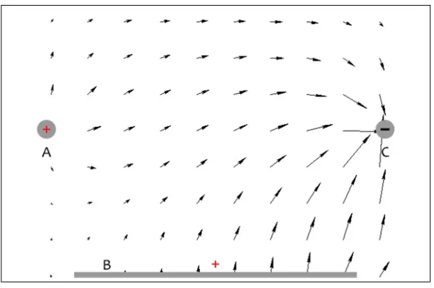
Figure 1 shows the design for a set of metallic rods and plate that will serve the purpose of

generating a non-uniform electric field (e-field). We will use the term “plates” or “e-field

generator” to collectively refer to the two rods and rectangular plate in figure 1. In the current

design, the plates have a length of about 5 millimeters and rods A and C, which are spaced apart

by ~2 millimeters, are both raised above plate B by 1 millimeter.

Fig 1

E-field generator consisting of three metal “plates,” A, B, & C. The plates are ~5 [mm] long. Distance between plates A & C is ~2 [mm]. Plates A & C are raised ~1 [mm] above plate B.

Another perspective of the depiction in figure 1 appears in figure 2 with an addition: between

the plates is a container that holds a mixture of electrolyte and at least one type of neutral

compound to be detected. At any given time, the electric field produced by the e-field generator

is activated in one of two states. The first state is what is shown in figure 2 and the second

appears in figure 3. Switching back and forth between the two states moves neutral molecules

that are contained within the field in a back and forth manner, as illustrated. An exemplary

figures is highly exaggerated. Provided below is further elaboration on the principles of

operation of the e-field generator.

Fig 2

E-field generator consisting of three metal “plates,” A, B, and C. Not drawn to scale. A sample container is positioned inside the generator. One of the plates is connected to the positive terminal of a voltage source and the other two plates are connected to the negative terminal of the voltage source. Configuring the connections this way results in one of two states of the non-uniform electric field.

Fig 3

E-field generator as in figure 2, except with reversed polarity on plate B. This reversal results in the second of two states of the non-uniform electric-field. Not drawn to scale.

The neutral molecule depicted in figures 2 and 3 has partial charge separation (δ+ _{and δ}-_{) or in}

other words, the molecule has a dipole. This dipole may be intrinsic or induced by the electric

blue and the solution is enclosed by an insulator (black outline) so that electric-current flow is

not possible from the plates into the solution.

A total of three plates comprise the e-field generator, of which two are rod-shaped and the third

is planar. The plates are respectively labeled A, B, and C in figures 1-3. The charge-polarity on

plates A and C are kept constant. That is, plate A remains positively charged and plate C remains

negatively charged when the electric field changes state. On plate B, however, polarity is

reversed between states. This reversal is in fact what creates the two e-field states. In the first

state (figure 2), plate B is negatively charged. In the second state (figure 3), it is positively

charged.

We now examine the two states of the electric field and their effects. In the first state, plate A

has greater charge density than plate C. Therefore, the electric field in the vicinity of plate A is

stronger than in the vicinity of plate C and the neutral analytes thereby migrate toward plate A,

as shown in figure 2. For the second state in figure 3, analytes migrate in the other direction

toward plate C where the electric is stronger. Simplified simulations of the electric for the first

Fig 4

Simplified electric-field simulation to illustrate the first state of the e-field generator. As the vectors show, the electric field is strongest at plate A. Simulation was performed with QuickFieldTM electrostatics software.

Second Phenomenon: Motion-Sensitive Saline

The first phenomenon described above was a method to induce motion of neutral molecules by

applying a non-uniform electric field. This section presents a second phenomenon: a

motion-sensitive electrochemical device that may be useful for detecting molecular motion. A simple

behavioral model for this device is provided based on both empirical observations and

literature research. This model will describe only some of the properties of the system. Other

unexplored properties of this motion-sensitive system are numerous and the objective of this

study is not to examine them exhaustively, but to apply some of the known properties in order

to assess the feasibility of a new molecular-sensor concept.

An example of a motion-sensitive device appears in figure 6, and is termed an

electrolyte-resistor voltage divider (ERVD). The ERVD consists of a DC voltage source, an electrolyte

solution (saline in this case) with two immersed electrodes, and a load resistor (RL). The

electrodes are made of copper or platinum in experiments presented below. The ERVD provides

an output voltage (Vout), as labeled in figure 6. This output voltage varies with mechanical

activity in the saline solution. Mechanical activity, that is, perturbation of the solution,

temporarily changes the effective resistance of the solution, thus modulating the output voltage.

The output voltage returns to its steady-state value when the disturbed solution is allowed to

settle.

The following discussion is an exploration of empirical attributes of an ERVD. From these

attributes, we develop a qualitative model for the system and then use this model to make a

refined prediction of system response to stimulation.

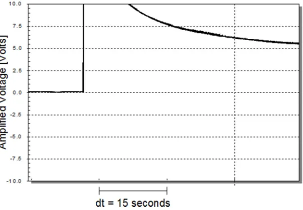
Figure 7 presents an exemplary output-voltage profile for an ERVD at the moment it is powered

on (when the voltage source is turned on). Output voltage jumps abruptly from zero to some

high value when the input DC voltage source is turned on. Over time (several minutes,

depending on configuration), this output voltage settles to an equilibrium value. Settling will

occur more quickly if the input voltage from the DC source is initially set to a high value, then

reduced to the operating value. Figure 8 shows the output voltage when the system has settled.

This equilibrium output voltage remains stable for the duration over which it is observed (more

than one hour).

Fig 8

ERVD at equilibrium. Screenshot shows ERVD output-voltage vs. time. Output-voltage is amplified 1000X. The ERVD Output-voltage source (Vsrc) is set to 0.1 [V] and RL is 1 [KΩ]. The electrolyte is saline and electrodes are made of copper. A 15-second interval is marked on the horizontal axis. Data acquisition rate is 100 [Hz]. Output-voltage

remained relatively stable for duration observed (more than 1 hour).

Figure 9 demonstrates what occurs when the saline solution is perturbed by vibrating the

solution container or by stirring the solution, for example. The output voltage increases, then

declines back to its equilibrium level as the solution comes to rest.

In light of the observations in figures 7-9 and based on fundamental concepts from

electrophoresis, a simple model for the ERVD can be developed that is suitable for the purposes

of this investigation.

To explain why the output voltage of an ERVD starts out and then settles to an equilibrium

value following power up, we consider that the saline solution contains ions that migrate in

response to voltage applied on the immersed electrodes. According to Wright [3, p. 276-277]

and other electrochemistry literature, Na+ _{and Cl}- _{are the main ions that flow in a saline solution}

when it is conducting electricity. In gel electrophoresis, a system that is similar in operation to a

saline conductor, ions can be visually observed to move under the influence of an applied

voltage, coming to a stop when they reach the electrode to which they have affinity. However,

the experimental results in figure 8 demonstrate that not all ions in solution migrate to the

electrodes. An appreciable current (~4 μA) continues to flow after the initial surge, indicating that ions remain in significant amounts throughout the solution.

Figures 7 and 8 thereby suggest that equilibrium is attained between the quantity of ions

stationed at the electrodes and the quantity of ions in the rest of the solution. When the ERVD is

initially powered, few ions are at the electrodes. Thus, ions begin to migrate to the electrodes,

causing the output-voltage surge seen in figure 7. As ions accumulate at the electrodes, the

concentration of ions at the electrodes hypothetically begins to approach a level that would not

be sustainable; consequently, the flow of ions to the electrodes levels off, corresponding to the

observed leveling of the ERVD output-voltage. Ion accumulation at the electrodes may be

described by a charge double-layer model [5] where the negatively- or positively-charged

electrode is complemented by ions of opposite charge from the electrolyte.

In figure 9, perturbing the solution appears to remove some of the accumulated ions at the

electrodes (disruption of double-layer), thereby causing them to flow back to the electrodes.

This return-flow generates additional current temporarily to restore the presumed charge

From this model, we can predict that the motion-sensitive property of an ERVD is localized to

its electrodes rather than the entire solution. This hypothesis was tested and the result appears

in figure 10. When an electrode is stroked with a non-conducting rod, as if to brush off ions

from the electrode, a sharp peak is observed. This stroking is performed twice to produce the

result in figure 10. In contrast, stirring the entire solution in this experiment produces a similar

result to that shown for the experiment in figure 9 – a broad peak is observed. These results are

consistent with the model of electrode-localized sensitivity. Perturbation at the electrodes

produces sharp, strong peaks; and perturbation away from the electrodes produces weaker,

broader peaks. If the perturbation occurs far enough from the electrodes, then no response is

observed.

Fig 10

ERVD experiment similar to the experiment in figures 7-9. Screenshot shows ERVD output-voltage vs. time with output-voltage amplified 1000X. The ERVD voltage source (Vsrc) is set to 0.1 [V] and RL is 1 [KΩ]. The electrolyte is saline and electrodes are made of copper. A 15-second interval is marked on the horizontal axis. Data acquisition rate is 100 [Hz]. One electrode of the ERVD is stroked twice with a non-conducting rod, producing a sharp peak for each stroke.

Combining the Two Phenomena

We have now described both a method to induce neutral-molecule motion and secondly a

whether these two phenomena can be combined effectively to create a sensor that will

quantitatively detect and identify neutral molecules. The proposed approach for this

combination is to prepare a mixture of electrolyte solution (ex. saline) that contains a small

amount of neutral analytes. This mixture is then analyzed in what we may designate a

“molecule motion sensor” (MMS), illustrated in figures 11 and 12. Below, we explore the

hypothetical operation of the MMS.

Fig 11

Molecule motion sensor (MMS), consisting of e-field generator and ERVD. The e-field is in the first of two states. Only the electrodes of the ERVD appear in the figure (load resistor and voltage source not shown). Not drawn to scale.

The MMS in figures 11 and 12 is comprised of an e-field generator and an ERVD. Not all

components of the ERVD are illustrated in the figures. As shown, ions accumulate at the

electrodes of the ERVD; and as described previously, the e-field generator creates a

non-uniform electric field with two possible states. Switching back and forth between these states

translates neutral molecules back and forth in the container. Figure 11 shows one state of the

electric field. Figure 12 shows the second state. Ionic molecules, on the other hand, do not

respond to the change in electric-field state in this simplified model. Ionic molecules ordinarily

remain stationary because charge polarity does not change at certain regions of the container,

for example in proximity to plates A and C. In other words, it is predicted that any free ion will

migrate toward a region that has a fixed charge polarity that is opposite to that of the ion and it

will remain there. However, the movement of neutral molecules in the container will tend to

perturb ions at the electrode, displacing them temporarily, as illustrated. The output voltage of

the ERVD would reflect this perturbation.

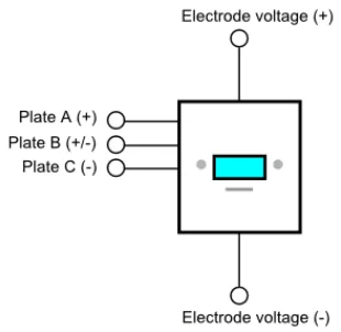
To further elaborate on the operation of the MMS, a schematic representation of the MMS is

presented in figure 13. The MMS has five electrical connections. The “Plate A (+)” terminal

connects plate A (ex. figure 12) to the positive node of a voltage source; the “Plate C (-)”

terminal connects plate C to the negative node of the same voltage source; and the

“Plate B (+/-)” terminal connects plate B to a signal that switches between the positive and

negative nodes of the voltage source. This switching occurs at an adjustable frequency. Finally,

the “electrode voltage (+)” and “electrode voltage (-)” terminals respectively connect the two

electrodes of the ERVD with the rest of the ERVD circuit. The ERVD circuit and the e-field

generator are connected to separate voltage sources, thereby preventing undesired

Fig 13

Schematic symbol for an MMS.

A pair of MMS devices may be employed for molecular analysis where one device contains the

sample to be analyzed (“sample cell”) and the other device serves as a reference (“reference

cell”). This configuration appears in figure 14. The output voltage (vout) for the pair is the

difference between the output voltages of the individual devices. This reference configuration is

chosen to mitigate artifacts that are not related to the nature of the analytes, and in essence

cancels out noise signal.

Maximizing MMS Sensitivity

In this section, we explore potential approaches for maximizing the sensitivity of the MMS

sensor pair in figure 14. Put another way, we will determine the conditions that will produce

the largest output voltage when minimum amounts of chemical are analyzed in the MMS. To do

so, we derive an expression for the output signal and inspect it for levers that can be adjusted to

maximize sensitivity. In figure 14, the output voltage is given by

=

−

, (1)

where Vsrc is the voltage of the power source as shown, RL is the value of the two identical load

resistors, rs is the effective resistance of the sample cell solution, and rr is the effective

resistance of the reference cell solution. Here, we have modeled the impedance of the

electrolyte solutions as a variable resistor, similar to small-signal analysis of transistors at an

operating point. For other applications, including scenarios where higher frequency signals are

employed, more complex models may be useful [6].

When the sample and reference cells are at rest, vout is ideally zero, resulting from the fact that rs

is ideally equal to rr under this condition. When both cells are probed with the two-state electric

field, the sample-cell electrodes will hypothetically be perturbed by the moving neutral analytes

in solution, whereas the reference-cell solution remains at rest because it contains only

electrolyte. As a result, rs decreases whereas rr does not change, thereby producing a positive

output voltage. As apparent in equation 1, the magnitude of the output voltage may be boosted

by using a larger value for Vsrc. This method is one possible way to increase the sensitivity of the

MMS. In practice, Vsrc cannot be made arbitrarily large. In the types of experiments that have

been conducted so far, Vsrc must be kept low enough to avoid currents in the milliamp range or

higher. Such large currents result in vigorous bubbling (gas release) in the saline solution,

creating undesired perturbation and altering the solution electrochemistry. This phenomenon

may well be a result of exceeding the electrochemical window of the water solvent [7]. In the

experimental setup employed below, the bubbling and sudden increase in current commences

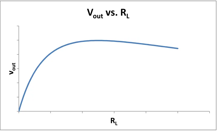
A second lever for maximizing sensitivity is to optimize the value of RL. Since RL appears in both

numerator and denominator of equation 1, predicting its effect on sensitivity is not as

straightforward as in the case of Vsrc. We thereby proceed by exploring how the output signal,

vout, changes with RL in order to find a value for RL that will generate the largest output signal.

Figure 15 is an exemplary plot of vout vs. RL when the sample cell is perturbed so that rs ≠ rr. The

values of rs and rr are fixed (held constant) in this simulated plot.

Fig 15

Exemplary simulated plot of vout vs. RL when rs ≠ rr.

From the plot in figure 15, we see that the function vout has a maximum. To calculate the value of

RL where this maximum occurs, we observe that the slope of the function vout is zero at the

maximum. Therefore, we can set the derivative (slope function) of vout to zero and solve for RL.

The derivative of vout with respect to RL is

=

( )

−

( )

. (2)

Setting this result to zero, we obtain

v

ou

t

R

_L

( )

−

( )

= 0

. (3)

Rearranging, we get

( )

=

( )

.

(4)

Solving equation 4 for RL, we obtain

=

∙

. (5)

From equation 5, we can see that the optimal value for RL is the geometric average of the

sample-cell and reference-cell resistances. Though, rr may be a fixed value, rs changes when the

sample solution is perturbed, resulting in a value of RL that varies in equation 5. Since a fixed

resistor will be used to implement RL in the circuit, we wish to calculate a single optimum value

for RL. We do so by optimizing RL for detecting weak perturbations, rather than any level of

perturbation. While this new value of RL may not be optimum for strong perturbations in the

sample cell, it will be good enough because the detection threshold of the sensor has been

minimized. To calculate this new value of RL, we take the limit of RL as rs approaches rr, the

condition for weak perturbation:

lim

→

= lim

→

∙

=

. (6)

We conclude that the optimal value for RL that will maximize the output signal is rr when there

is only weak perturbation. In other words, we adjust the value of RL in the circuit until half the

supply voltage falls across the RL resistors (RL = rr = rs at equilibrium). Intuitively, it makes

sense that the function vout will have its maximum at RL = rr: examining equation 1, if RL is too

small or approaching zero (RL << rr), then the output will also approach zero. If on the other

hand RL is too large (RL >> rr), then the output will again go to zero. Thus, the maximum for vout

Analysis Concepts

We now examine concepts that underlie the process of identifying and quantifying molecules in

a sample using an MMS as the analysis tool. These concepts are: the relative quantity of analytes

in the electrolyte solution of an MMS and the attenuation of molecular swing at high

frequencies. After describing these concepts, we will proceed to demonstrate how they come

into play in detecting molecules and measuring their concentration.

Relative Quantity of Analytes in Electrolyte Solution

Referring to figure 14, the sample cell of an MMS contains a mixture of electrolyte solution and

neutral compounds (“analytes” or “sample”). The reference cell contains only electrolyte

solution. Therefore the output signal of the MMS ideally represents the difference in

composition between the two cells. In order to minimize secondary effects such as changes to

the conductivity of the electrolyte solution, the relative quantity of analytes in the sample cell is

kept small, for example 1% or less. Using small quantities of sample may prevent significant

variation in the properties of the electrolyte solution from one experiment to the next when

different types of samples are analyzed. Additionally, small quantities of sample minimize

intermolecular interactions between analyte molecules so that each molecule behaves

independently of others at various concentrations. This independence promotes a linear

correspondence of analyte concentration with output signal.

Attenuation of Molecular Swing at High Frequencies

As shown in Figures 11 and 12, an electrode is positioned at each end of the container. If the

electrodes are made of platinum, one is far more sensitive than the other. The sensitive

electrode generates a significant positive voltage at the output when perturbed; whereas the

relatively insensitive electrode slightly reduces the output voltage when there is a disturbance

(negative contribution to the output). Neutral molecules translate from one end of the container

to the opposite end when the electric-field changes state, thereby perturbing the solution. This

back and forth change in state occurs at an adjustable frequency. At low frequency, perturbation

is not significant and therefore there is little output. At mid-range frequency, a large positive

output signal is detected. If the frequency is high enough, the molecules will not have sufficient

migration is initiated at the other electrode. As frequency continues to increase, the distance

traversed by the molecules per cycle will also decrease. This reduction in swing will

hypothetically result in diminished perturbation of ions at the sensitive ERVD electrode; thus,

output voltage falls. Figure 16 illustrates a hypothetical frequency sweep of the MMS sensor.

Fig 16

Hypothetical result of frequency sweep in an MMS pair comprised of a sample and a reference cell.

Referring to figure 16, frequency is swept from low to high value rather than from high to low

value. This approach eliminates the settling time that would otherwise be required for the

electrolyte solution if transitioning from higher to lower frequencies.

In figure 16, the sensor output reaches a maximum then begins to decrease. The range of

frequencies where the output reverses direction and begins to decrease may be described as an

“attenuation range.” Assuming that the analyzed sample in figure 16 contains only one type of

molecule, then the observed attenuation range may be characteristic of that compound. That is,

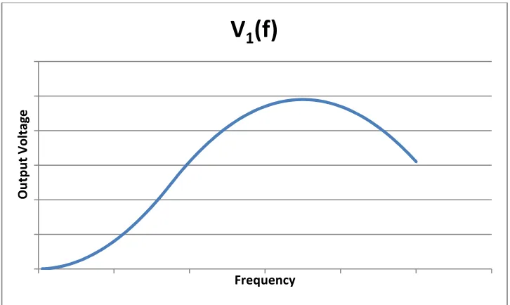
different types of molecules may attenuate at unique frequency ranges. Figure 17 provides

hypothetical examples of spectra for two different types of molecules (“molecule 1” and

O u tp u t V o lt a g e Frequency

“molecule 2”). Each of the two spectra attenuates at a different set of frequencies: V2(f), the

spectrum of molecule 2, begins to decline when the output for molecule 1, V1(f), is still

increasing.

Fig 17

Two conceptual output signals, V1(f) and V2(f). V2(f) initially has a greater magnitude than V1(f) but attenuates earlier than V1(f).

The attenuation range of a molecule is presumed to be related to its ability to quickly respond

to the state-switching electric field. Molecules that can move quickly will resist attenuation,

resulting in an output that only declines at high frequencies. Slow-moving molecules are not

able to respond as quickly to the state change and therefore may not traverse the extent of the

container to reach the sensitive electrode. They therefore attenuate early at low frequencies.

The agility of a molecule in the electric field depends on its properties including mass, shape,

dielectric constant or dipole magnitude, and extent of intermolecular interaction with the

surrounding medium (drag). Heavy and wide molecules with a weak dipole will tend to move

slowly, whereas small molecules with a strong dipole would move quickly.

Standard Sample Approach

Based on the concepts described above, what we expect in the MMS is a sensor whose output is

linear with respect to concentration (not illustrated) but has a nonlinear frequency response

(ex. figure 16). Presented in this section is a method to extrapolate molecule concentration and

identity by processing raw signals such as those modeled in figures 16 and 17. This method

would be particularly useful in the situation where the sample to be analyzed contains more

than one type of chemical, resulting in a complex raw signal in which a distinct signature for

each molecule is difficult to ascertain. We may refer to this method as the “standard sample

approach” (SSA).

The essence of the SSA is to employ the spectrum of a known chemical(s) at a known

concentration to decipher the spectrum of an unknown sample. The known chemical serves as a

comparative standard and hence is the “standard sample.” Suppose the spectrum of the known

sample is given by the function K(f) and that of the unknown sample is given by U(f). We may

determine the identity and concentration of molecules in the unknown sample by deriving a

quotient function Q(f) given by

Q(f) =

%(&)_'(&). (7)

Essentially, we have divided the spectrum of the unknown sample point for point by the

spectrum of the known sample. If for example, Q(f) = 1 at all frequencies, this result would

indicate that the known and unknown samples are probably identical: they contain the same

chemical(s) at the same concentration(s). In another example, if Q(f) = 0.8 across all

frequencies, we can conclude that both samples are proportionally composed of the same

chemical(s), but the concentration of the unknown sample is 80% that of the known sample.

Figures 16 and 18 aid in illustrating this concept. V1(f) appears in figure 16 and in figure 18, K(f)

Fig 18

A linear quotient function resulting from comparison of chemically similar samples. The unknown and known samples differ only in analyte concentration.

In general, a test sample that proportionally contains the same chemicals as the standard

sample but at a different concentration may have a spectrum U(f) given by

U(f) = c · K(f), (8)

where c is the concentration of the test sample relative to the standard sample. In this case, Q(f)

= c. The absolute concentration of the test sample in terms of a specific unit may be obtained by

multiplying c by some conversion factor α, where α is a constant.

In another scenario where the standard sample and unknown sample have dissimilar chemical

constituents, suppose that K(f) is equal to V1(f) in figure 16 and U(f) = V2(f) in the same figure.

Assume V1(f) and V2(f) are spectra for two different types of molecules, molecule 1 and

molecule 2. The two compounds have different attenuation ranges. The quotient function is

given by

Q(f) =

%(&)_'(&)

=

,(&)

,-(&). (9)

0 0.2 0.4 0.6 0.8 1 O u tp u t R a ti o , Q (f ) Frequency

A plot of Q(f) appears in figure 19 below.

Fig 19

Quotient function resulting from comparison of chemically dissimilar samples. The unknown sample attenuates earlier than the standard sample.

As the plot of Q(f) in figure 19 is not a straight line, we can conclude that the standard sample is

chemically dissimilar to the unknown sample. The relative concentration of the unknown

sample (molecule 2) can still be obtained. Molecule 2 attenuates before molecule 1, hence the

quotient function declines in value. We can obtain the relative concentration of molecule 2

before this decline occurs by taking the value of Q(f) at a low frequency. In the case of figure 19,

c = 1.5. The absolute concentration of molecule 2 may be expressed as β·c, where β is a constant

that depends both on the unit of concentration employed and on the behavior of molecule 2 in

the sensor. The identity of molecule 2 may be determined by observing its attenuation pattern

and frequency range in Q(f).

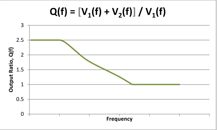
Figure 20 presents another scenario. Here, the quotient function is similar to that in figure 19,

except that it has a higher initial value and attenuates to a value of 1, instead of 0 as in figure 19.

0 0.5 1 1.5 2 O u tp u t R a ti o , Q (f ) Frequency

Fig 20

Varying quotient function resulting from comparison of a solution containing two types of molecules and a solution containing only one of the compounds.

We may interpret Q(f) in figure 20 to represent a sample that is a mixture of molecule 1 and

molecule 2. At low frequencies, both compounds contribute to the output. At higher

frequencies, molecule 2 attenuates and no longer contributes to the output. In this case,

Q(f) =

,-(&) ,(&)

,-(&)

= 1 +

,(&)

,-(&). (10)

When V2(f) diminishes to zero, Q(f) = 1, as figure 20 illustrates. The relative concentration of

molecule 1 is calculated by taking the value of Q(f) after attenuation of molecule 2; in this case,

Q(f) = 1. Similarly, the relative concentration of molecule 2 may be calculated by subtracting the

concentration of molecule 1 from the total concentration: 2.5 – 1 = 1.5. Thus, the relative

concentration of molecule 2 is 1.5. The same technique may be applied to analyze any unknown

sample with spectrum U(f), provided that each type of molecule in the sample has a distinct

attenuation range. Where attenuation ranges overlap, other techniques such as observing

changes in slope and the frequencies where the changes occur may be employed to both

identify the molecules and determine their concentration. Figure 21 is a plot of a quotient

function for a hypothetical sample that contains three analytes in addition to a standard sample.

0 0.5 1 1.5 2 2.5 3 O u tp u t R a ti o , Q (f ) Frequency

Attenuation ranges for each type of molecule is marked in the figure, with molecule types 1 and

2 having overlapping ranges in part of the spectrum.

Fig 21

Quotient function where unknown sample contains three types of analytes in addition to chemical(s) in the standard sample.

Nested Sweeps of Electric Field and Frequency to Discover Attenuation Ranges

The strength of the electric field between the plates of the e-field generator has a direct impact

on the speed of analytes as they migrate from one wall of the solution container to the opposite

wall. If molecules are moving so quickly that attenuation is not observed within the frequency

arrange available for a sweep, the electric-field strength may be lowered in order to slow down

the molecules. A systematic approach for discovering attenuation ranges of analytes would be

to perform nested sweeps: the electric-field strength is set to an initial level and then a

frequency sweep is performed. The electric-field strength is then increased and another

frequency sweep is performed. This process may be repeated as necessary. Fast-moving

molecules would hypothetically be detected at low field strengths whereas under the same

conditions, slow-moving molecules will produce weak signals and may not be detected. In

molecules will exhibit detectable swing attenuation. For a given analyte, each step increase in

the electric-field strength may produce at most one attenuation range.

Experiments

This section presents experimental results from testing the above hypotheses. We proceed by

briefly describing the methods of the experiments and then follow with results. In the next

section, we discuss conclusions drawn from the results.

In each experiment, a sample containing analyte is placed in the sample cell of an MMS pair; and

a sample containing only saline is placed in the reference cell. The analyte in the sample cell

constitutes 1% of the sample solution by mass. This sample solution is prepared by mixing 0.1

[g] of analyte with 9.9 [g] of saline solution. The stock saline is prepared by adding distilled

water to 50 [g] of salt (NaCl) for a total solution volume of 250 [mL]. Experiments are

conducted at room temperature. RL for both sample and reference cells is set to 250 [KΩ]. Vsrc is

set to 4.15 [V] so that rs and rr, which vary with Vsrc, are ≅ 250 [KΩ] at equilibrium. The voltage

between Plate A and Plate C is 2400 [V]; and Plate B switches between 2400 [V] and 0 [V],

thereby creating the time-varying electric field. The switching frequency of the field starts at

100 [Hz] and increments by 100 [Hz] for the next data point, with the frequency sweep ending

at 5 [KHz]. In the plots, Δ vout (“delta vout”) on the y-axis is the change in vout rather the actual

value of vout.

Figure 22 is a photo of the sample and reference cells, which are separated by an impermeable

wall. The cells are made of WaterShed XC 11122 material and manufactured by FineLine

Prototyping, Inc using 0.002” resolution stereolithography. Both cells are recessed at the

bottom. The sensing electrodes are housed in these 1 [mm]-deep recesses and are 99.95%

platinum metal. Appendix E covers cell configuration.

In experiments, both cells are filled with 1 [mL] of solution and then the ERVD circuit is

powered on. After approximately 1 minute of settling, 700 [μL] of solution is removed from each cell and a lid is placed over the recess in the cells. The lid is made of the same material as

the cells. Once the sensor output settles again, data acquisition commences. From empirical

detector sensitivity several fold, possibly by increasing ion accumulation at the electrodes. The

excess volume is then removed prior to data acquisition. Removal of this excess volume after

settling does not noticeably alter sensitivity.

Fig 23

Saline vs. Saline spectrum. Both the sample and the reference cells of the sensor contain only saline solution in this control experiment. The point sampled at frequency 3600 [Hz] is not shown in the plot as it is an extreme, random outlier most likely caused by generated bubbles that burst.

Fig 24

1% Isopropyl Alcohol (IA) vs. Saline Spectrum. Data from analysis of 1% isopropyl alcohol in the sample cell and saline in the reference cell. The point sampled at frequency 3700 [Hz] is not shown in the plot as it is an extreme, random outlier most likely caused by a generated bubble that burst.

-160 -140 -120 -100 -80 -60 -40 -20 0

0 1000 2000 3000 4000 5000 6000

Δ Vo u t [μ V ] Frequency [Hz]

Saline vs. Saline Spectrum

-180 -160 -140 -120 -100 -80 -60 -40 -20 0

0 1000 2000 3000 4000 5000 6000

Δ Vo u t [μ V ] Frequency [Hz]

Fig 25

1% Glucose vs. Saline Spectrum. Data from analysis of 1% glucose in the sample cell and saline in the reference cell. The points sampled at frequencies 1700 [Hz] and 4600 [Hz] are not shown in the plot as they are extreme, random outliers most likely caused by generated bubbles that burst.

Fig 26

1% Glycerol vs. Saline Spectrum. Data from analysis of 1% glycerol in the sample cell and saline in the reference cell.

-200 -150 -100 -50 0 50

0 1000 2000 3000 4000 5000 6000

Δ Vo u t [μ V ] Frequency [Hz]

1% Glucose vs. Saline Spectrum

-300 -250 -200 -150 -100 -50 0

0 1000 2000 3000 4000 5000 6000

Δ Vo u t [μ V ] Frequency [Hz]

Fig 27

Quotient function of two spectra of 1% glycerol vs. saline. The sample cell contains 1% glycerol and the reference cell contains saline. The same sample set is analyzed twice in the sensor in order to perform a sensor consistency check.

Discussion

In some of the data presented, one or two data points were not included in the plot as they

are outliers. These outliers are not considered relevant because they are most likely caused by

bubbles that burst in the sample or reference cell, resulting in undesired perturbation. The

bubbles arise from gases that form at the electrodes.

Perhaps the most pertinent observation in reviewing the data in figures 23-26 above is that the

change in output voltage (delta vout) is negative rather than positive. This result squarely

contradicts expectations and suggests a systematic artifact. As the sample cell of the sensor

contains analyte and the reference cell does not, we would expect a positive output voltage.

Further scrutiny of the sensor performance and additional experimentation is required to

either confirm or invalidate the above results.

In much of the data (except the glucose analysis), the output follows a trend of becoming

increasingly more negative. However, as this trend also holds in the control experiment of

0 0.5 1 1.5 2 2.5 3

0 1000 2000 3000 4000 5000 6000

O u tp u t R a ti o , Q (f ) Frequency [Hz]

figure 23, it is more than likely only an artifact as opposed to related to the nature of the

analytes. The contents of the sample and reference cells are identical in the control experiment:

they both hold saline only.

In light of the unexpected results, it was important to determine at the minimum whether the

sensor readings were consistent. One approach was to analyze a particular sample twice and

compare the data from both readings point by point. The plot in figure 27 above is an example

of this comparison: we obtain the quotient function for two spectra from a 1% glycerol vs.

saline experiment. We would expect this quotient function to have a value of 1 across all

frequencies. We nearly obtain this result in figure 27. This outcome largely holds for other

experiments. We can thus conclude that despite the negative output of the sensor, it performs

fairly consistently.

If the relatively weak artifact-signals are ignored, then in effect the sensor has zero output; that

is, the applied electric field does not induce detectable molecule motion. This result may stem

from a number of factors. One important factor is the electric-field strength. The applied

transient electric field may not be sufficiently strong to induce molecular motion, considering

the types of compounds that were assayed. Past experiments leading up to this study and those

by Tsori et al [1], have either exclusively analyzed nonpolar molecules or a combination of

nonpolar and polar molecules. In contrast, the experiments presented here exclusively analyze

polar molecules (water, glucose, glycerol, isopropyl alcohol). As a result of their polar nature,

these compounds are expected to less readily separate under the influence of an electric field.

A lack of significant output signal from the sensor precludes analysis of attenuation ranges or

determination of concentration. In summary, the detector function (ERVD) of the sensor is

operational; however, the effectiveness of the e-field perturbation scheme requires further

investigation.

Future Studies

One experimental approach to scrutinize the above results while minimizing the possibility of

artifacts is to design a simpler prototype where the electric field pattern is altered mechanically,

electric fields without generating potentially interfering signals. The objective of this simplified

experiment would only be to determine whether a transient electric field has an unmistakable

impact on an ERVD output. More elaborate experiments can follow if the result is positive.

A large number of factors come into play in the MMS. For example, a variety of electrolytes may

be employed in an MMS and may each produce unique results to allow unambiguous

identification of more compounds. The mechanism of current flow in select electrolyte solutions

may be examined further. The size and shape of the ERVD electrodes possibly are important

variables that affect ion accumulation and thus sensitivity. It may also be useful to determine

various analytical relationships, for example, the effect of electric-field strength on the

attenuation range of an analyte and the impact of changes in temperature. Miniaturization of

the MMS system from millimeter to micrometer scale is another consideration. These factors

may be explored in future studies. Improved methods for precisely perturbing the ERVD

REFERENCES

[1] Tsori Y, Tournilhac F, Leibler L. Demixing in Simple Fluids Induced by Electric Field

Gradients. Nature 2004; 430: 544-547

[2] Tsori Y, Leibler L. Phase-Separation in Ion-Containing Mixtures in Electric Fields. PNAS

2007; 104 (18): 7348-7350

[3] Wright, Margaret Robson. 2007. An Introduction to Aqueous Electrolyte Solutions. John

Wiley & Sons Ltd, England.

[4] Kremer F, Schönhals A. 2003. Broadband Dielectric Spectroscopy. Springer-Verlag,

Berlin, Germany.

[5] Koryta J, Dvorak J, and Kavan L. 1993. Principles of Electrochemistry. 2nd _{ed. p. 198-244.}

Wiley Publishers, Chichester, England.

[6] Webster J. 1997. Medical Instrumentation: Application and Design. 3rd _{ed. p. 183-200.}

John Wiley & Sons Ltd, Hoboken, New Jersey.

[7] Bockris J, and Reddy A. 1998. Modern Electrochemistry I: Ionics. 2nd _{ed. p. 720. Plenum}

APPENDIX A – System Design Overview

The electronics for the molecule-sensor prototype consist of a computer (PC), a data acquisition

device (DAQ) controlled by software on the PC, and a custom-designed circuit (CC). The data

acquisition device is a LabJack U3 (labjack.com). Descriptions of the main functions of each

component are in table 1 below.

Table 1

Overview of Molecule-Sensor System Design

PC DAQ Custom Circuit (CC) • Determine next switching

frequency in frequency sweep

• Signal DAQ to generate digital clock signal for selected frequency • Send signal to tare CC

output, if necessary • Sample data point at the

new frequency • Repeat above at next

frequency



• Handle

communication between PC and CC (AD and DA conversions) • Generate

square-wave switching signal (clock) at frequency specified by PC • Generate analog

offset voltages for CC amplifier circuit



• Use clock signal from DAQ to switch electric-field across sample

• Power ERVD

• Amplify signal from sensing electrodes

• Filter high frequency noise • Pass signal to DAQ for AD

conversion

APPENDIX B – Circuit Schematics

Schematics for the sensor custom circuit (CC) appear below. The circuit has two main divisions.

One division mediates generation of the state-switching electric field and the second division

detects and amplifies output signal from the ERVD pair. The two divisions are electrically

isolated to minimize interference. Additional data for selected components appear in

Appendix C.

Figures 28-30 show overlapping snapshots of the first division of the circuit. The following is a

description of this division of the circuit and the functions of its key components.

Fig 28

Circuit mediating generation of state-switching e-field. Zoom for detail. Schematic is continued in figures 29 and 30.

In one clock cycle, M1 charges the Plate B node to a high voltage (up to 2.4 KV). In another clock

cyle, M2 discharges the Plate B node. Both M1 and M2 are NMOSFET. Ordinarily, M1 would be

available. To isolate other parts of the circuit from high voltage, the gates of M1 and M2 are

charged via photocouplers (photo-electric switches) designated Phc3 and Phc4 in figure 29.

Fig 29

Circuit mediating generation of state-switching e-field. Zoom for detail. Schematic is a continuation of figure 28 above and culminates in figure 30 below.

As M1 is NMOS rather than PMOS, it is necessary to reference the Plate B node when applying a

gate-source voltage. Since the Plate B node carries a high voltage, the power source for M1

requires isolation. This power source is implemented with a local capacitor (C3) in order to

avoid loading the Plate B node with stray capacitance from wiring, which would severely reduce

switching frequency. When C3 is depleted, it is recharged via a DPDT relay (Rel1) that connects

C3 to a 12 [V] DC power source. The relay disconnects both leads of C3 from the DC supply

when charging is complete in order to prevent loading the Plate B node with stray capacitance.

Phc5 is a photocoupler that controls Rel1. Phc5 receives a digital signal from the DAQ device to

ZD1 is a zener diode connected to the gate and source of M1 and prevents damage to M1 from

stray high voltage discharge. R23 and R24 keep M1 and M2, respectively, completely off when

not activated by preventing buildup of trace gate-source voltages.

The switching photocouplers Phc3 and Phc4 each contain two separate photo-electric switches

for a total of four switches. The decade counter, IC1 (figure 28), generates four digital signals

(Q0-Q3) that control these switches, respectively. Only one switch in activated in a given cycle.

For each transistor, one switch charges Cgs (the gate-source capacitance) and a second switch

discharges it. With this switching mechanism, no overlap exists between the on-times of M1 and

M2, thus avoiding a short-circuit current. R1 and R3 (figure 29) work as a voltage divider that

provides an output that is one-thousandth the voltage at Plate B. This lower voltage makes it

possible to monitor the high voltage on Plate B.

Fig 30

Circuit mediating generation of state-switching e-field. Zoom for detail. Schematic is a continuation of figures 28 and 29 above.

The component HVP5P (figure 30) is a high-voltage power supply and can deliver up to 1 [mA]

of current. Its positive output connects to the Plate A node of the MMS (figure 13) and its

adjustable and is set in this circuit by one of four selectable potentiometers (CT1 – CT4). Phc1

and Phc2 are photocouplers that select which potentiometer is active. SW0-SW4 are digital

select lines from the DAQ device that activate the corresponding photocoupler unit in Phc1 or

Phc2. C4 stabilizes the output of HVP5P.

Figures 31 and 32 are schematics for the second division of the sensor circuit. This part of the

circuit powers the ERVD pair and amplifies the output signal. In figure 31, the components

labeled PL2 and PL3 respectively connect the two electrodes of the sample cell and the two

electrodes of the reference cell to the circuit. Connected to both PL2 and PL3 are variable

resistors (CT6 – CT9) for setting the value of RL in both branches. Using two variable resistors in

each branch allows for coarse and fine adjustment of RL. Switches SW5a and SW5b disconnect

the variable resistors from the circuit when their values are to be measured and set.

Fig 31

ERVD circuit with signal amplifiers, noise filter, and ERVD power source. Zoom for detail.

Amp1 is an instrumentation amplifier that amplifies the difference between the outputs of the

ERVD pair by a factor of 100. The reference pin of Amp1 (pin 5) allows the output of the

the output of the amplifier. Taring is performed when the signal from the ERVD pair exceeds

the range of the amplifiers. Applying an offset voltage brings the signal back into range,

provided that the signal does not exceed the available offset. Both the offset voltage and the

amplifier output are recorded. During data analysis, the offset is subtracted from the modified

sensor output in order to regain the true signal.

The Amp2 IC houses two separate op-amps, Amp2a and Amp2b. Amp2a amplifies the signal

from Amp1 by another factor of 100 for a total gain of 10,000. R15 and R16 set the gain of

Amp2a and C2 turns the amplifier into a low-pass filter to eliminate high frequency noise.

Sources of noise include background RF and the state-switching electric field in the first

division of the circuit. Amp2b is simply a voltage buffer for monitoring the output of Amp1

without degrading the signal.

Amp3, like Amp2, is actually two separate op-amps on one IC (Amp3a and Amp3b). Amp3a

serves as a variable voltage source for the ERVD pair. Its output voltage is set by the

potentiometer labeled CT5. Capacitor C1 suppresses noise that may otherwise arise in the

op-amp output, thus creating a stable DC voltage supply. Amp3b is a voltage buffer for monitoring

the output of the reference cell. Its input is connected to the node labeled “R Set 2,” the output of

the reference cell.

Fig 32

Circuit supplying offset voltage to Amp1. Zoom for detail.

Figure 32 is a schematic of the circuit that creates the offset voltage that is fed into Amp1 in

figure 31. The nodes DAC0 and DAC1 are the outputs (with respect to ground) of two variable

and the other is fed into its negative input. With this configuration, both positive and negative

offset voltages can be created, depending on the settings of these voltage sources. R17 – R20

comprise voltage dividers that scale the DAC0 and DAC1 voltages down to manageable levels

and also increase voltage-step resolution for finer control of the offset voltage.

Fig 33

Summary of relevant inputs and outputs of the custom circuit. Zoom for detail.

Figure 33 organizes the most relevant inputs and output signals of the entire circuit. The first

four inputs (“+12V Amp” through “-12V Amp”) are pins for two DC power supplies for the

amplifiers. The “Earth” pin grounds the high-voltage circuit that creates the two-state electric

field. “12V HV+” and “12V HV-“ are power-supply input pins for the high-voltage source, HVP5P.

DAC0 and DAC1 are connections for software-controlled voltage sources on the DAQ device.

They are referenced to the node “DAQ Gnd.” SW0 – SW3 are digital signal lines from the DAQ

device, only one of which is activated at a time; they control the output voltage of the

high-voltage source, HVP5P, selecting from up to four pre-set high-voltages. “DAQ 5V” and “DAQ Gnd” are

the supply rails from the DAQ devices. “DAQ 5V” delivers 5 [V] with respect to “DAQ Gnd.” Clock

is the digital frequency signal from the DAQ device and drives the state-switching of the electric

field. The “Relay” digital signal turns relay Rel1 on or off.

For the outputs, “Amp Out” is the amplified, noise-filtered signal from the ERVD pair. “Pre Amp

Out” outputs the signal from the first amplification stage for monitoring purposes. “Ref C Out”

outputs the signal from the reference cell for monitoring. Q3 is for monitoring the state of the

electric field. “HV Pulse Mon” outputs a scaled-down facsimile of the pulsed high-voltage that

e-field generator circuit and is typically connected to an oscilloscope. “HVMonitor” allows

monitoring of the high-voltage DC output of HV5P via a lower, more manageable voltage. Plates

A-C connect to the MMS circuit board, which houses the sample and reference cells (figure 22).

Electrode plugs PL2 and PL3 (shown in figure 31) also connect to the MMS circuit board,

APPENDIX C – Component Reference

Table 2

Lookup Reference for Specialized Components

Circuit Designation Description Manufacturer Part Number/Name

IC1 Decade counter NXP Semiconductors HEF4017B

Phc1- Phc4 Photocoupler (switch) Vishay Semiconductors ILD1

Phc5 Photocoupler (switch) Toshiba TLP626

M1, M2 4KV NMOSFET IXYS Corporation IXTV03N400S

HVP5P DC 5KV voltage source Pico Electronics HVP5P

Rel1 Mechanical relay TE Connectivity D3222

Amp1 Instrumentation amp Analog Devices AD620B

Amp4 Instrumentation amp Analog Devices AD620A

APPENDIX D – Software Code

Software that runs on a computer controls the DAQ. The DAQ may be programmed via this

software. Below are the routines (code) that comprise the program for the current sensor

implementation. The name of the routine or function appears above each printout. Zoom to

enlarge images.

Table 4

Routine: main

Table 6

Function: freq_out()

Table 7 continued

Table 9

Function: readPoint()

Table 11

Sub-routine: saveData()

Table 12

Sub-routine: set_hv_level()

APPENDIX E – Cell Configuration

Fig 34

Simulation of the first state of the electric field, including the electrodes. The effects of the solution and the small potential applied to the electrodes by Vsrc are not included in the simulation. The simulation was performed with QuickFieldTM electrostatics software.