Behind the Scene of Side Channel Attacks

(1)

Behind the Scene of Side Channel Attacks

— Extended Version —

Victor Lomn´e, Emmanuel Prouff, and Thomas Roche

ANSSI

51, Bd de la Tour-Maubourg, 75700 Paris 07 SP, France

{firstname.lastname}@ssi.gouv.fr

Abstract. Since the introduction of side channel attacks in the nineties,

a large amount of work has been devoted to their effectiveness and ef-ficiency improvements. On the one side, general results and conclusions are drawn in theoretical frameworks, but the latter ones are often set in a too ideal context to capture the full complexity of an attack performed in real conditions. On the other side, practical improvements are pro-posed for specific contexts but the big picture is often put aside, which makes them difficult to adapt to different contexts. This paper tries to bridge the gap between both worlds. We specifically investigate which kind of issues is faced by a security evaluator when performing a state of the art attack. This analysis leads us to focus on the very common situation where the exact time of the sensitive processing is drown in a large number of leakage points. In this context we propose new ideas to improve the effectiveness and/or efficiency of the three considered attacks. In the particular case of stochastic attacks, we show that the existing literature, essentially developed under the assumption that the exact sensitive time is known, cannot be directly applied when the latter assumption is relaxed. To deal with this issue, we propose an improve-ment which makes stochastic attack a real alternative to the classical correlation power analysis. Our study is illustrated by various attack experiments performed on several copies of three micro-controllers with different CMOS technologies (respectively 350, 130 and 90 nanometers).

1 Introduction

(2)

and formal statements (sometimes at the cost of too simple models), many of the practical analyses only focus on a particular attack specificity and often put the big picture aside. The latter analyses are indeed usually dedicated to one specific attack running against a specific target device, which makes them hard to generalize. This paper tries to be at the intersection of both worlds: we study practice-driven issues while keeping a generic approach w.r.t. attacks mechanisms and targeted platforms. This approach and our final purpose are close to those in the works of Standaertet al.[38] and Renauld et al.[33].

The starting observation of our study is that side channel traces are never reduced to one point in practice, even when they rely on the manipulation of a single variable. In contrary, those traces are often composed of a large number of points (typically several thousands). In spite of the evidence of this observation, it is rarely taken into account when analysing the effectiveness of a side chan-nel attack. Such an analysis is indeed frequently done under the assumption, sometimes implicit, that a small number of points of interest (POI) has already been extracted from the traces either by pattern matching [22], or by dimension reduction [1, 6, 7, 37] or thanks to a previous successful attack [10, 33]. However, the two first categories of techniques are not yet perfect and, after reduction, the traces are often still composed of several points in practice. And, what is more important, the risk of information loss during the reduction process leads most of attack practitioners to not apply them. The third technique (performing a first attack to identify the POI) allows for interesting analyses, but it does not correspond to areal attack context. Moreover, the best POI for one attack type may not be so good for another one. Eventually, we come to a situation where attacks are analysed in a (uni-dimensional) context which does not fit with the (multi-dimensional) reality faced by the attack practitioners.

We argue in this paper that the state-of-the-art uni-dimensional analyses cannot be straightforwardly adapted to multi-dimensional contexts, which raises new interesting issues. The selection of the most likely candidate among the re-sults of several instantaneous attacks is one of them. Indeed when the leakage traces are composed of several points, a side channel attack against the targeted sensitive variable must be performed for each point (a.k.a time index) in the traces. Then, the adversary must apply a strategy to select the most likely can-didate among the different instantaneous attacks results. A classical method is to select the one with the highest score (e.g.the highest correlation coefficient in a Correlation Power Analysis – CPA– [8]). Nevertheless we argue that this strategy can be ineffective for some attack categories, including the case of the Linear Regression Analysis (LRA) [11,35,36]. For the latter one, we propose a new strategy to select the most likely candidate and we demonstrate its effectiveness in practice.

(3)

with this goal in mind. A common structure in their algorithmic description is exhibited and then used to propose a new general modus operandi which en-ables to significantly reduce the computation time when the number of traces is non-negligible.

Finally, to make sure that our analysis is consistent with the reality, we completed our investigations by several experiments performed on three micro-controllers based on different CMOS technologies (350,130and90nanometers process). We report here on these experiments results. We moreover use them to confirm and complete the interesting behaviours observed in [33]: (1) the leakage seems to diverge from the classical Hamming weight model as the CMOS technology tends to the nanometer scale, which makes LRAa promising tool for side channel evaluations of nano-scale devices and (2)TAis effective in practice, even when the templates are built on one copy of the device and the attack is done on another copy.

The paper is organized as follows. In Section 2, we introduce the theoretical background for our study and we present the outlines of our proposal. Then, three sections are dedicated to the application of our ideas to theLRA,CPAandTA re-spectively.

2 SCA: Practical Issues

In this section, we introduce some basics and we get into the specifics of the problematic focused in this paper.

2.1 Notations

Throughout this paper, random variables are denoted by large letters. A real-ization of a random variable, said X, is denoted by the corresponding lower-case letter, said x. A sample of several observations of X is denoted by (xi)i.

It will sometimes be viewed as a vector defined over the definition set of X. The notation (xi)i ←- X denotes the instantiation of the set of observations

(xi)i fromX. Themean ofX is denoted E[X], its standard deviation byσ[X]

and its variance by var[X]. The latter equals E(X−E[X])2. The

covari-ance of two random variables X and Y is denoted by cov(X, Y) and satisfies cov(X, Y) =E[(X−E[X])(Y −E[Y])]. When we will need to specify the

vari-able on which statistics are computed, we will write the varivari-able in subscript (e.g. EX[Y] instead ofE[Y]).

(4)

2.2 General Attacks Framework

In this paper, the attacks framework is described by considering that the adver-sary targets the manipulation of a single sensitive variableZ, but the study and results directly extend to contexts where several variables are targeted in par-allel. The variableZ is supposed to functionally depend on a public variableX and a secret sub-partksuch thatZ =F(X, k) whereF is a (n+n, m)-function (which impliesX, k∈Fn2 andZ∈Fm2 ). The bit-lengthsnandmdepend on the cryptographic algorithm and the device architecture1.

The attacks are described under the assumption that the adversary ownsN side channel traces −→`0, ...,

− →

`N−1, each of them containing information about Z. Namely, the ith _{leakage trace} −→_`

i ←

-− →

L corresponds to the processing of a public value xi ←- X and contains information on the value zi ←- Z such

that zi = F(xi, k). The dimension of the traces (i.e. the number of different

instantaneous leakage points) is denoted byd. By definition, we haved= dim. −→L. When little information is known about the implementation and the device (which is usually the case in practice), the exact manipulation time ofzi cannot

be precisely determineda priori. Also, precision in the observation often comes at the cost of a high sampling rate2_{. As a consequence, the dimension of the traces is} usually high (from several thousand of points up to millions) and the attack must be repeated on all of their coordinates independently (as e.g.in CPA and LRA) or must consider huge traces chunks globally (as e.g.forTA). Although bearing differences, the three latter attacks follow a common process flow (see Algorithm 1 below). Starting from this generic description, this paper studies, in Sections 3, 4 and 5 respectively, theeffectiveness and efficiency of theCPA,LRAandTA at-tacks. The core ideas of those analyses are presented in the two next sub-sections.

1. Pre-processing on the observations−→`i.

,→extract statistics from the traces.

2. Pre-processing on the predictionsF(xi,kˆ) for all ˆk.

,→extract statistics from the predictions based on a model and/or

an estimation of the leakage statistics conditioned by the values of the manipulated data.

3. Processing on the predictions and observations.

,→compute a distinguishing valuefor each key hypothesis and each

instantaneous leakage time of each observation.

4. Return a key candidate.

,→select the key candidate with the maximum distinguishing value

over all the instantaneous leakages times.

Algorithm 1: Generic Attack Flow

1 _{An example of function}_F_{is the function that applies a so-called}_sbox_{transformation}

to the bitwise addition betweenkandX.

2

(5)

2.3 Effectiveness Discussions

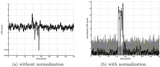
A part of our study is dedicated to thedistinguisher value definition and, more precisely its relevance when considering side channel traces with a large number of points. This study was motivated by the observation that the classicalLRA dis-tinguisher value for one leakage time is not comparable as such to that computed for another leakage time. Figure 1(a) illustrates this claim for anLRAtargeting the device B described in Section 2.5: when directly applying the protocol given in [11, 36], the correct key candidate does not maximize the distinguisher value globally but only in a local area, which makes the attack unsuccessful unless this area is known by the adversary (which is not assumed here). This observation led us to study the handling of distinguishing values inSCAattacks. We for in-stance show that by normalizing the LRAdistinguishing values, the correct key candidate becomes clearly distinguishable even when considering the full vector of instantaneous attack results (as depicted on Figure 1(b)).

0 50 100 150 200 250 300 350 400 0.9999

0.9999 1 1 1 1 1 1 1 1

time points

LRA score

(a) without normalization

0 50 100 150 200 250 300 350 400

0 2 4 6 8 10 12 14 16

time points

normalized LRA score

(b) with normalization

Fig. 1. InstantaneousLRA scores computed over 10000 traces (scores for the correct

key in black)

More generally, our study relies on a well studied problem which is the com-parison of the results of two different instantaneous attacks [11, 21, 38, 39, 41,43]. For theLRA, it will lead to a modification of the candidate selection rule.

2.4 Algorithmic Complexity Improvements Proposals

(6)

imple-mentations can easily reach several days of processing and this is not compatible with standard evaluation processes3_.

We show in Sections 3, 4 and 5 that the three considered attacks may be re-written in a partitioningfashion that can be exploited to significantly decrease the algorithmic complexity. Roughly speaking, the basic idea is to lower the im-pact of the heavy computations (i.e.Algorithm 1, Step 3) so that its complexity does no longer depend on the traces number N but on the dimension n of the targeted data. To that purpose, we propose to modify the attack first step so that it processes separately the traces with respect to their input valuexi. As a

result, the algorithmic complexity of the attacks Step 3 is divided by ₂Nn making

the algorithmic improvement interesting whenN 2n (which is often the case in practice). The improved generic attack flow is summed up in Algorithm 2.

1. Partitioning of theN observations−→`iaccording to the valuesxi. ,→extract statistics for each of the 2n _partitions.

2. Pre-processing on the predictionsF(xi,ˆk) for all ˆk.

,→extract statistical data from the key hypothesis and plaintext based on the function F and a model and/or an estimation of the leakage statistics.

3. Processing on the predictions and traces statistics.

,→compute a distinguishing valuefor each key hypothesis and instantaneous leakage based on the pre-processed statistics.

4. Return a key candidate.

,→select the key candidate with the best distinguishing valueover all the instantaneous leakages

Algorithm 2:Improved Generic Attack Flow

Almost every SCA may be rewritten as a combination of tests on statistics estimated on leakage partitions. Some of them (e.g.theDPA[18] or the multi-bit

DPA[24]) were actually originally written as such, whereas the other ones were developed in a partitioning way after their introduction (see e.g. [19] for the

CPA, [10] for the LRAand [38] for the MIA). To the best of our knowledge, this property has however never been exploited to improve the attacks efficiency.

2.5 Experimental Setup

For each studied SCA, practical experiments were performed on three Micro-Controller Units (MCUs for short) with different CMOS technologies (350, 130 and 90 nanometers processes). The observed processing was that of an AES128 encryption handling one byte at a time. Each attack was performed against 4

3 _{In Common Criteria evaluations applied on hardware security devices, all}

(7)

sbox outputs of the first round. Furthermore, to measure the variability of our experiments, we used three different copies for each MCU (called copy 1, 2 and 3 in the sequel). This choice enabled us to perform theTAprofiling step on one copy and to use the results to attack other ones. Also, it gives more credit to our experimental results as the templates consistency was checked on three different versions of the same MCU.

The side channel observations were obtained by measuring the electromag-netic (EM) radiations emitted by the device. To this aim, several sensors were used, all made of several coils of copper (the diameters of the coils were respec-tively of 1mm, 500µm and 250µm for the 350, 130 and 90nm MCUs), and were plugged into a low-noise amplifier. To sample measurements, a digital oscillo-scope was used with a sampling rate of 1G samples per second for the 350nm MCU and 10G samples per second for the others, whereas the MCUs were run-ning at few dozen of MHz.

We insist on the fact that the temporal acquisition window was set to record the first round of the AES only. This synchronization has been done thanks to

simple electromagnetic analysis[30]. As the MCU clocks were not stable, we had

to resynchronize the measurements. This process is out of the scope of this work, but we emphasize that it is always needed in a practical context and it impacts the measurements noise.

We sum-up the specificities of the three experimental campaigns hereafter: – Device A (3 copies): 90nm CMOS technology with MCU based on a 8-bit

8051 architecture. EM traces composed of 12800 points each after resynchro-nization. Highest Signal to Noise Ratio (SNR) over the full traces equals to 0.09.

– Device B(3 copies): 130nm CMOS technology with MCU based on a 8-bit 8051 architecture. EM traces composed of 16800 points each after resynchro-nization. Highest SNR equals to 0.6.

– Device C(3 copies): 350nm CMOS technology with MCU based on a 8-bit AVR architecture. EM traces composed of 51600 points each after resyn-chronization. Highest SNR equals to 0.3.

3 Practical Evaluation of Linear Regression Attacks

(8)

Section 2.3 is thus put aside. Moreover, the question of the efficient processing of the attack, when applied against high dimensional leakage traces, is not tackled. The rest of this section aims at dealing with two issues.

3.1 Attack Description

InLRA, the adversary chooses a so-called basisof functions4₍

mp)16p6swith the

only condition that m1 is a constant function (usually m1 = 1). Then, for each xi and each sub-key hypothesis ˆk, the prediction ˆzi = F(xi,ˆk) is calculated.

The basis functionsmp are then applied to the ˆzi independently, leading to the

construction of a (N ×s)-matrix Mˆ_k = (. mp(F(xi,ˆk))i,p. The comparison of

this matrix with the set of d-dimensional leakages (−→`i)i6N ←

-− →

L is done by processing a linear regression of each coordinate of−→`iin the basis formed by the

row elements ofMˆ_k. Namely, a real-valued (s×d)-matrixBˆ_kwith column vectors −

→

β1,· · ·,−→βdis estimated in order to minimize the error when approximating

− →

`>_i by (m1(F(xi,ˆk)),· · · ,ms(F(xi,ˆk)))× Bˆ_k. The matrix Bˆ_k is defined such that:

Bˆ_k= M>ˆ_k × Mˆk

−1 × M>ˆ_k

| {z }

Pˆk

×L , (1)

whereLdenotes the (N×d)-matrix with the−→`>_i as row vectors. In the following, the uth column vector ofL (composed of the uth coordinate of all the −→`i) is

denoted by −→L[u]. Moreover, the (s×N)-matrix M>

ˆ

k × Mˆk

−1 × M>

ˆ

k, which

does not depend on the leakage values, is denoted by Pˆ_k.

To quantify the estimation error, thegoodness of fit model is used and the

correlation coefficient of determination R2 _{is computed for each} _u_{. The latter}

is defined by R2 _{= 1}₋_SSR_/_{SST, where SSR and SST respectively denote}

the residual sum of squares (deduced from Bˆ_k) and the total sum of squares5

(deduced fromL). We give in Algorithm 3 the pseudo-code corresponding to a classical LRA attack processing.

3.2 On the LRA Effectiveness

Let us focus on the best candidate selection step in a classicalLRA. Each sub-key hypothesis ˆkis first associated with a score which is the greatest instantaneous

coefficient of determinationwhen testing it for all temporal coordinates u. It is

denoted by maxuR[ˆk][u] in Alg. 3. The second phase of the selection consists

in the processing of the maximum argmaxˆ_k(maxuR[ˆk][u]). The purpose of the

latter step is to identify the candidate that maximises the greatest instantaneous coefficient. Implicitly, such a classical approach by total maximisation of the

distinguisher value assumes that the most likely candidate corresponds to the

4

The basis choice and its impact are not a trivial matter, see [10] for a detailed study.

5

(9)

Algorithm 3: LRA- Linear Regression Analysis

Input : a set ofd-dimensional leakages (→−`i)i6Nand the corresponding plaintexts

(xi)i6N, a set of model functions (mp)p6s

Output: A candidate sub-key ˆk

/* Processing of the leakage Total Sum of Squares (−−→SST) */

1 fori= 0toN−1do

2 µ→−

L =µ→−L+

− →

`i

3 σ→−

L=σ→−L+

− →

`2_i

4 −−→SST =σ−→

L−1/N·µ

2

− → L

/* Processing of the2n _{predictions matrices} _M

ˆ

k andPˆk */

5 forˆk= 0to2n₋₁_do

/* Construct the matrixMˆk andPˆk */

6 forp= 1tosdo

7 fori= 0toN−1do

8 Mˆk[i][p]←mp[F(xi,ˆk)]

9 Pˆk= (M

>

ˆ

k × Mˆk)

−1_{× M}>

ˆ k

/* Test hyp.ˆk for all leakage coordinates */

11 foru= 0tod−1do

/*Instantaneous attack (at time u) */

12 →−β =Pˆk×

− →

L[u]

/* Compute an estimator−→E of −→L[u] = (−→`0[u],· · ·,

− →

`N−1[u])> */

13 →−E=Mkˆ×

− →

β

/*Compute the estimation error (i.e. the SSR) */

14 SSR = 0

15 fori= 0toN−1do

16 SSR = SSR + →−E[u]−−→`i[u]2

/* Compute the coefficient of determination */

17 R[ˆk][u] = 1−SSR/−−→SST[u]

/* Most likely candidate selections */

18 candidate = argmaxˆk(maxuR[ˆk][u])

(10)

greatest value taken by the distinguisher not only over all sub-key hypotheses but also over all the leakage times. This assumption relies on another one, often done in the embedded security community, which states that the value of a distinguisher computed between wrong hypotheses (i.e.computed for a wrong sub-key value or a wrong time) and the leakage values tends toward its minimum value (often 0) when the sample size N increases (see e.g. [21]). However, as already noticed in several papers (e.g.by Messerges in [24], Brieret al.in [8] or by Whitnal et al. in [45]), both assumptions are often not verified in practice, where the adversary must for instance deal with the ghost peaks phenomenon. The situation is even worst for the LRA attacks since the vector of coefficients −

→

β (and thus the set of predictions) depends not only on ˆk but also on the attack time 6 u. The strength of the LRA, namely its ability to adapt to the instantaneous leakage, is also its weakness as it makes it difficult to compare the different instantaneous attacks results.

To illustrate the issue raised in the previous paragraph, we experimented a LRAagainst an AES sbox processing running on Device B (see Section 2.5). The full leakage traces were composed of 16800 points. We performed the attack on the full trace length and, for each time coordinate, we recorded the scores of all the 256 key-candidates after N = 1000 observations. For clarity reasons, we present in Figure 2 the results only for a temporal window of size 250 points where the targeted variable was known to occur. In the top of the figure, the rank of the correct key is plotted and it can yet be observed that it is 0 for few times. In the second trace of Figure 2, the instantaneous maximum scores comprised in [0.9982,0.999] are plotted7: it may be checked that the maximum among those scores corresponds to a time (t= 238) when the correct key is not ranked first. This explains why the total maximisation approach fails in returning the correct key candidate in this case.

To build a better rule than the total maximisation test, we respectively plot-ted in the third and fourth traces of Figure 2 the mean (plain green trace) and the variance (plain red trace) of the instantaneous scores (i.e. the values µ(u) = 2−8P

ˆ

kR[ˆk][u] and σ(u) = 2

−8P ˆ

k(R[ˆk][u]−µ(u))

2 _with _u _denoting the time coordinate in abscissa). For each time, we also plotted in black dashed line, the maximum score max(u) = maxˆ_k(R[ˆk][u]). It may be observed that the correct key is ranked first at the time u when the distance max(u)−µ(u) is large andσ(u) is small. The third (red) trace and the fourth (gray) trace aim at supporting this claim. Eventually, they suggest us the following pre-processing before comparing the instantaneous attack results: for each leakage coordinate, center the maximum of the coefficients of determination and divide it by their standard deviation. The resulting scoring is plotted in the fifth (magenta) trace, where it can been checked that the maximum is indeed achieved for the correct key.

6 _{As recalled in Section 4, it is not the case for the}_CPA_{as the predictions}_m₍_F₍_x,_ˆ_k₎₎

are the same for each instantaneous attack

7

(11)

50 100 150 200 250 0

100

200

rank

50 100 150 200 250

0.9982 0.9984 0.9986 0.99880.999

max & mean

0 50 100 150 200 250

0 2 4x 10

−9

variance

0 50 100 150 200 250

0 2 4x 10

−4

max−mean

0 50 100 150 200 250

0 5 10x 10

5

time points

(max−mean)/var

Fig. 2.LRAon Device B (over 1000 traces): Scores Statistics

As a conclusion, and in the light of our analysis, we propose to replace the candidate selection step of theLRAby the following ones8_:

18 foru= 0tod−1do

19 attackRes[u] ={argmaxkˆ R[ˆk][u]

,maxˆk R[ˆk][u]

−E_ˆ

k

R[ˆk][u]

σ_ˆ

k

R[ˆk][u] }

20 candidate = arg1max2 attackRes

In Section 3.4, our scores pre-processing technique is applied to attack sam-ples of Device A and Device C in order to test whether our observations, about (1) the ineffectiveness of the classical LRA and (2) the soundness of the new pre-processing, stay valid for other devices than Device B.

3.3 On the LRA Efficiency

The construction of the prediction matrices in Alg. 3 implies, for each ˆk, the processing of 3 products of matrices with one dimension equal to s (number of basis functions) and the second dimension equal to N (number of leakage traces). The processing of the instantaneous attacks also requires two such matrix products for each pair (ˆk, u) withu₆d. This makes the application of a linear regression attack as depicted in Alg. 3 difficult to perform (and even impossible)

8 _{where arg1max2 is a function returning the first coordinate of the maximum of an}

(12)

when the numberN of leakage traces and/or the number dof attack times are large. Fortunately this complexity can be significantly reduced. It can indeed be easily shown (see [10]) that the processing of the vectors −→β is unchanged if performed for the set ofaveraged leakages(_#_{_i_:_x1

i=x}

P

i,xi=x

− →

`i)x∈Fn2 instead of

(−→`i)i. Actually, this amounts to change the definition of the matricesMˆ_kandL

in (1) such thatMˆ_k= (. mp(F(x,kˆ))x∈Fn2,p6sandLis a (2

n_×d_{)-matrix whose}_xth

row vector−→L>_[_x_{] equals} 1 #{xi=x}

P

i,xi=x

− →

`i. This improvement essentially lets

the first 9 steps of Alg. 3 unchanged except the loop 7-8 which is now computed over x∈_Fn

2 instead of overi ∈[0;N −1]. Then, before Step 10, the following processing is done to compute the elements of the matrixL:

for i= 0toN−1do

−→ L>_[_x

i] =

−→ L>_[_x

i] +

− →

`i

count[xi] = count[xi] + 1

forx= 0to2n−1do

−→

L>_[_x_{] =}−→_L>_[_x_]_/_count[_x_]

Eventually, Steps 10-17 are replaced by the following ones where we recall that −→L[u] denotes theuth column vector ofL.

for ˆk= 0to2n−1do

/* Test hypothesisˆk for all leakage coordinates */

foru= 0tod−1do

/* Instantaneous attack (at timeu) */

− →

β =Pˆk×

− →

L[u]

/* Compute an estimator−→E of −→L[u] = (L[0][u],· · ·,L[2n−1][u])> */

− →

E=Mkˆ×

− →

β

/* Compute the estimation error (i.e.the residual sum of squares) */

SSR = 0

forx= 0to2n₋₁_do

SSR = SSR + →−E[x]− L[x][u]2

/* Compute the coefficient of determination */

R[ˆk][u] = 1−SSR/−−→SST[u]

The efficiency improvements proposed here for the LRAattack allows for a significant time/memory gain. First, it replaces the (N×s)-matrix products at Step 13 by (2n_×_s_{)-matrix products. More globally, the complexity is reduced}

from O(s×d×N) to O(s×d×2n_{). A detailed counting of the elementary}

(13)

the matrix products Mˆk× Pˆk can also be pre-processed. This enables to save

one matrices product per loop iteration (over ˆkandu).

3.4 Experiments

We experimented the classical and improved LRA against against three copies of Devices A, B and C (see Section 2.5). The attacks target four bytes of the AES state after the first SubBytes operation and they are applied on the full side channel traces. Each attack has been performed 10 times against each of the three copies. The average rank over the four correct sub-keys is plotted in Figure 3 for each device. We recall that the rank of a sub-key kis here defined as the position of maxuR[k][u] in the vector (maxuR[ˆk][u])_kˆafter sorting (see Section 2.2 for a discussion about this choice). The experiments reported in Figure 3(a)-(c) are done with alinear basis(i.e.the functionsmi were chosen such thatm0is constant equal to 1 andmi, withi68, returns theith bit of its inputs). It may

be observed that the classical attack always failed whereas the improved one succeeded with less than 2500 observations (and even less than 800 for Device B). After noticing that the attack was less efficient on Device A (90nm) than that on Device B (130nm), we chose to perform a new attack campaign against the former, but this time with a quadratic basis (i.e. the functions corresponding to the product of two input bits were added to the linear basis). Results are given in Appendix C (Fig. 9) and it can be noticed that we did not witness any effectiveness improvement.

500 1000 1500 2000 2500 3000 3500 4000 0

20 40 60 80 100 120 140 160

number of traces

average rank of the correct key

LRA normalized LRA

(a)LRA on Device A

100 200 300 400 500 600 700 800 900 1000 0

20 40 60 80 100 120 140 160

number of traces

LRA normalized LRA

(b)LRAon Device B

100 200 300 400 500 600 700 800 900 1000 0

20 40 60 80 100 120 140 160

number of traces

LRA normalized LRA

(c)LRAon Device C

Fig. 3.LRAcampaign – Rank evolutionversusnumber of observations

(14)

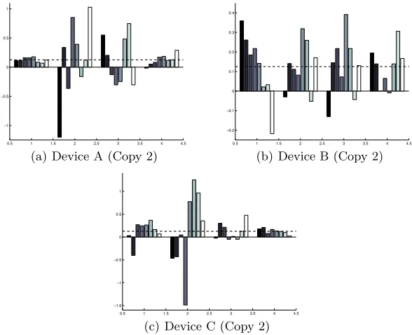
comparison, we also plotted in blue dashed line the value corresponding to the normalized weight (i.e. 1₈) of a bit in a Hamming Weight model. For Devices A and C, it may be noticed that the first and fourth sbox output manipulations leak closely to the Hamming weight model (normalized weights are more or less balanced). This is not the case of the weights of the second and third sbox outputs, which are very unbalanced. For Device B, one can observe that at least two bits leak significantly less than the others.

0.5 1 1.5 2 2.5 3 3.5 4 4.5

−1 −0.5 0 0.5 1

(a) Device A (Copy 2)

0.5 1 1.5 2 2.5 3 3.5 4 4.5

−0.2 −0.1 0 0.1 0.2 0.3 0.4

(b) Device B (Copy 2)

0.5 1 1.5 2 2.5 3 3.5 4 4.5

−1.5 −1 −0.5 0 0.5 1

(c) Device C (Copy 2)

Fig. 4.LRAweights for each of the 3 devices

4 Practical Evaluation of Correlation Power Analysis

Correlation Power Analysis was proposed by Brieret al.[8] in 2004. The idea is to use Pearson’s correlation coefficient as a distinguisher instead of the difference of means test originally proposed by Kocher et al. [18]. CPAis certainly nowa-days the most popular side channel technique as it proved itself (combined with classical leakage models like the Hamming weight and Hamming distance) very efficient on an overwhelming majority of hardware architectures9. The naturally good effectiveness of CPAwas already mentioned in Brieret al.paper as the use

9

(15)

of CPAallows to reduce the presence ofghost peaks compared to classical DPA. Subsequent works on CPA effectiveness essentially consisted in applying signal filtering techniques or pre-processing on the leakage traces (seee.g.[6, 26] for re-cent works on this subject). We do not propose amelioration here on this topic. About the attack efficiency, very few works dealt with this problem at the algo-rithmic level. In fact, published works on this subject have essentially addressed the issue of processing theCPAon multicore CPU or graphic processor unit (see

e.g.[4]). We show in this section that re-writing theCPAas in a partitioning way allows for a significant efficiency gain. This re-writing has already been proposed in [19] but, to the best of our knowledge, it has never been used for efficiency improvement purpose10.

In a correlation power analysis attack, the adversary computes, for each plaintext xiand each sub-key hypothesis ˆk, an hypotheses tuple ˆzisuch that ˆzi=F(xi,ˆk).

Then, he chooses a so-calledmodel function m(·) fromFm2 intoRand applies it to each hypothesis which leads to the construction of a new set of so-called

predictions (hi)i6N ←

-− →

H = m(F(X,kˆ)). This latter set of hypotheses is then compared to the set of leakages (−→`i)i6N ←

-− →

L to assess on the likelihood of ˆ

k as a candidate for one of the sub-keys k. The core principle of a CPA is to make the comparison by estimating the linear correlation between −→H and each coordinate of−→L independently. We give in Alg. 4 the pseudo-code corresponding to theCPAattack discussed previously. A brief description of it may also be found in Appendix B.

4.2 On the CPA Effectiveness

Based on the discussion conducted in Section 3.2 and the success of the experi-mental validation of the new selection strategy, this may seem natural to try it in theCPAcontext. However, the fact that the same constant modelm(·) is used for each instantaneous attack (which was not the case for theLRA) implies that two correlation coefficients corresponding to two different coordinates of the vectors −

→

`iare directly comparable (since they are quantifying the linear correlation

be-tween the leakages and a common model). Therefore the most likely hypothesis corresponds to the greatest value of the correlation coefficient/score when the set of hypotheses (ˆzi)iis tested with respect to each coordinateuof the vectors

− →

`i. We actually checked that the normalizing strategy applied in Section 3.2

indeed does not enable to improve theCPAefficiency.

10

(16)

Algorithm 4: CPA- Correlation Power Analysis

Input : a set ofd-dimensional leakages (−→`i)i6N and the corresponding

plaintexts (xi)i6N, a model functionm(·)

/* Leakage mean and variance processing */

1 fori= 0to N−1do

2 µ−→

L =µ−→L+

− →

`i

3 σ−→

L =σ−→L +

− →

`2i

4 µ−→

L = 1/N·µ→−L

5 var−→

L = 1/N·σ→−L −µ−→L

2

/* Hypotheses mean and variance processing */

6 forkˆ= 0to2n₋₁_do

7 fori= 0to N−1do

8 z←m(F(xi,kˆ))

9 µˆk=µkˆ+z

10 σ_kˆ=σˆ_k+z2

11 µˆ_k=µ_kˆ/N

12 varkˆ=σˆk/N−µkˆ

2

/* Correlations processing */

13 forkˆ= 0to2n₋₁_do

/* Test hypothesis ˆk for all leakage coordinates */

14 foru= 0 tod−1do

/* Instantaneous attack (at time u) */

15 cov = 0

16 fori= 0to N−1do

17 cov = cov +m(F(xi,kˆ))×

− →

`i[u]

18 cor[ˆk][u] = (1/N×cov−µkˆ×µ→−L[u])/ q

varˆk×var−→L[u]

19 candidate = argmaxkˆ(maxucor[ˆk][u])

(17)

4.3 On the CPA Efficiency

The law of total expectation implies:

cov(X, Y) =EE X−E[X] Y −E[Y]|X ,

where the conditional means are viewed as random variables that functionally depend onX. Due to the linearity of the mean, this latter equation is also equiv-alent to cov(X, Y) = E(X−E[X])E(Y −E[Y])|X. When applied in the

context of the correlation coefficients computation in Algorithm 4, this equa-tion leads to a significant efficiency improvement. Prior to Steps 13-18 in Alg. 4 (instantaneous attacks), we propose to insert the following pre-processing in order (1) to partition the leakage traces−→`i according to the corresponding

in-put valuesxi and (2) to compute the mean for each partition. We denoted by

A−→

L the matrix whose x

th _{column vector equals the mean of the elements in} {−→`i;xi=x}.

/* Conditional Leakage Averaging for each possible x */

EraseA−→

L

fori= 0 toN−1do

A→−

L[xi] =A→−L[xi] +

− →

`i

count[xi] = count[xi] + 1

forx= 0 to2ndo

A→−

L[x] =A−→L[x]/count[x]

Eventually, Steps 18-28 in Alg. 4 are replaced by the following ones where, for each of the 2n _{instantaneous attacks, the proposed efficiency improvement}

essentially allows for the replacement ofN−1 additions and multiplications by 2n ones. Taking the leakage conditional averaging step into account, this gives a replacement of d×2n×(2N + 6) elementary operations11 by 2N + 2n plus d×2n×(2n + 6). A detailed counting of the elementary operations for each attack is given in Appendix A.

4.4 Experiments

We experimented the classical and normalized CPAagainst the same targets as those used in Section 3.4. For both attacks, we used the classical Hamming weight function for m(·). Similarly as in Section 3.4, average ranks have been computed. They are plotted in Figure 5 for each device. It may first be noticed that theCPAis very efficient against Devices B and C as it respectively succeeds, on average, in less than 400 and 300 traces. The same attack against Device A

11

(18)

/* Correlations processing */

forˆk= 0to2n−1do

/* Test hypothesis ˆk for all leakage coordinates */

foru= 0 tod−1do

/* Instantaneous attack (at time u) */

cov = 0

forx= 0 to2n₋₁_do

cov = cov +m(F(x,ˆk))× A−→ L[x][u]

cor[ˆk][u] = (1/N×cov−µˆk×µ→−L[u])/ q

varˆk×var−→L[u]

is much less efficient (it requires around 9000 traces to succeed). This is a conse-quence of the low measurements SNR and the fact that the leaking information is not always well captured by the Hamming weight model (see Fig. 4(a)). Also, and as expected from our analysis in Section 4.2, the normalizedCPAis, on aver-age, not better than the classicalCPA. The relative ineffectiveness of the former with respect to the CPAseems to be all the more important than the SNR is small. Confirming this in other contexts could be of interest for further research. Eventually, theCPAon device A is less efficient than theLRAattack on the same device.

In the following two figures, we detail the evolution of the ranks of the four different targeted sub-keys in function of the numberNof observations. For each of them we only consider the rank at the time coordinate where theCPAfinally succeeds.

Figure 6(a) must be studied together with theLRAexperiments reported in Figure 4(a). It may indeed by observed that theCPAattack is particularly efficient against the manipulations that leak close to the Hamming weight (bytes 0 and 3) and lose efficiency for the two other bytes (1 and 2). Surprisingly (at a first glance), this phenomenon cannot be observed for Figures 6(b) and 4(c). Actually, this is a consequence of the fact that CPA and the LRAdo not always succeed for the same time coordinate. The unbalancedness observation made for 4(c) is therefore not relevant to interpret the results in 6(b). This is a consequence of the fact that theCPAsub-keys ranking evolution and the leakage characterisation correspond to different leakage times (in other words, the best leakage time for theLRAand theCPAdo not equal for Device C).

5 Practical Evaluation of Template Attacks

(19)

mea-1000 2000 3000 4000 5000 6000 7000 8000 9000 10000 0

20 40 60 80 100 120 140 160

number of traces

CPA normalized CPA

(a)CPA on Device A

100 200 300 400 500 600 700 800 900 1000

0 20 40 60 80 100 120 140 160

number of traces

CPA normalized CPA

(b)CPAon Device B

100 200 300 400 500 600 700 800 900 1000 0

20 40 60 80 100 120 140 160

number of traces

CPA normalized CPA

(c)CPAon Device C

(20)

1000 2000 3000 4000 5000 6000 7000 8000 9000 10000 0

20 40 60 80 100 120 140 160

number of traces

mean of the rank of the correct key

byte 0 byte 1 byte 2 byte 3

(a)CPA on Device A

100 200 300 400 500 600 700 800 900 1000

0 20 40 60 80 100 120 140 160

number of traces

mean of the rank of the correct key

byte 0 byte 1 byte 2 byte 3

(b) CPAon Device C

Fig. 6.CPAcampaign – Rank evolutionversusnumber of observations for the four sbox

outputs

surements (to go from time domain to frequency domain) and then by applying dimension reduction techniques (e.g.PCA). The latter idea is also followed in [1] and [3]. In all those papers, the improvement of the template attacks efficiency is not studied at the algorithmic level. Moreover, the reported template attack experiments involve the same device for the profiling and matching phases of the attacks, which strongly reduces the practical significance of the argumen-tations. Indeed, as the profiling phase requires a full access to the device (and in particular the ability to chose the secret parameter), the latter experiments do not fit with the large majority of real attack/evaluation contexts where the adversary has no (or very few) control on the target device. In a more realis-tic attacker model the profiling phase is conducted on a different device. For such a model, we have the following well known question about the efficiency of template attack: how sound/relevant is a profiling done on a device A when attacking another device B ?12_{The first work, and to the best of our knowledge,} the single one reporting on template attacks in such context is due to Renauld

et al.[33]. On the latter article, the two devices used for the experiments are test

chips implementing an AES s-box and made in 65-nanometer CMOS technology. The results presented in the rest of this section improve the state-of-the-art recalled previously on two points. First, the efficiency improvement is done at the algorithmic level. It can hence be combined with the previous improvements which essentially correspond to measurements traces pre-processing. Secondly, the reported experiments concern a full AES implementation running on 3 differ-ent samples of 3 differdiffer-ent technologies. This allowed us to complete the analyses done in [33] and to draw, for the first time, conclusions about the template attack efficiency for realisitic scenarios.

12

(21)

A template attack (TAfor short) assumes that a preliminary profiling step has been performed on an open copy of the targeted device. During this phase, the adversary has measured N0 _{leakage traces}−→_`

i

0

for which he knows exactly the values taken by the corresponding sensitive value Z (which also implies that he knows the corresponding sub-keyk). Those leakages have then been used to compute estimationsfz(·) of theprobability density functionof (

− →

L |Z=z) for all possible z (which imposesN0 2m_{). The pdf estimations} _f

z(·) will play in

a template attack, a similar role as the model functions in aCPAorLRA.

Once the adversary has the set of pdf estimations (fz(·))z∈Fm2 in hand, a TAagainst the set of traces (−→`i)i6N (for which the secrets are unknown) follows

essentially the same outlines as theCPAor theLRA: the hypothesis ˆkis tested by first computing the predictions ˆzi=F(xi,kˆ) and then by calculating the product

Q

i6Nfˆzi(

− →

`i). Usually, the pdf of the variables (

− →

L |Z =z) is estimated by a multivariate normal law, which implies thatfz can be developed s.t.:

fz(

− →

`i) =

1 (2π)d_det _Σ

z

exp −1 2

− →

`i− −→µz

>

Σ_z−1 −→`i− −→µz

, (2)

whereΣzdenotes the (d×d)-matrix of covariances of

− →

L |Z=zand where the (d)-dimensional vector−→µzdenotes its mean.

To minimize approximation errors induced by the processing of the product of exponential values, one usually prefers, in practice, a log-maximum likelihood processing to the classical maximum likelihood13. Together with (2), this leads to the following computation to test the hypothesis ˆk:

ML[ˆk] =−X

i6N

− →

`i− −→µˆzi

> Σ_z−_ˆ1

i

− →

`i− −→µzˆi

−X

i6N

log((2π)d+1det Σˆzi)

. (3)

We give in Alg. 5 the pseudo-code corresponding to theTAattack discussed previously.

13

(22)

Algorithm 5: TA- Template Attacks

Input : a set ofd-dimensional leakages (→−`i)i6Nand the corresponding plaintexts

(xi)i6N, a set of pdf estimations (−→µz, Σz)z∈Fm₂

/* Pre-Processing of the2m log-determinantslog(2πd+1Σz) and inverse-matricesΣ−_z1

*/

1 forz= 0to2m−1do 2 logDet_z= log(2πd+1Σz)

3 invCovz=Σ−z1

/* Instantaneous TA attacks Processing */

4 forˆk= 0to2n−1do

/* Test hyp.ˆk */

5 ML[ˆk] = 0

6 fori= 0toN−1do

7 ˆz=F(xi,ˆk)

8 ML[ˆk] =ML[ˆk]− −→`i− −→µzˆ>×invCovzˆ×

− →

`i− −→µzˆ−logDetˆz

9 candidate = argmaxˆk(maxML[ˆk])

10 returncandidate

5.2 On the TA Effectiveness

The idea developed in previous sections to improve the selection of the best can-didate among the results of several instantaneous attacks is not relevant here. Indeed, for both the profiling and attack phases, a template attack exploits, by nature, all the leakage coordinates of the −→`i simultaneously. There is

con-sequently no need to compare the results of several (different) instantaneous attacks.

5.3 On the TA Efficiency

Applying the same idea as for the CPA and the LRA, we propose hereafter an alternative writing ofML[ˆk] that leads to a much faster attack processing. For such a purpose, we focus on the term −→`i− −→µzˆi

> Σ_z−_ˆ1

i

− →

`i− −→µzˆi

in (3). After denoting byLi each (d×d)-matrix (

− →

`i[u]

− →

`i[u0])u,u0, we get the

fol-lowing rewriting of the latter term:

X

u,u0

Li[u][u0]×Σz−ˆi1[u][u

0_]

− −→µ>zˆi× Σ

−1 ˆ

zi +Σ

−1 ˆ

zi

>

×−→`i+−→µ>zˆi×Σ

−1 ˆ

zi × −

→_µ ˆ

zi .

After recalling that ˆzi equals F(xi,kˆ) and after denoting F(x,ˆk) by ˆz and

#{i, xi =x}byNx, we deduce that the sumP_i

− →

`i− −→µzˆi

> Σ−_ˆ_z1

i

− →

`i− −→µzˆi

(23)

X

x∈Fn2



 X

u,u0

X

i,xi=x

Li[u][u0]×Σ_z−_ˆ1[u][u0]

−−→µ>_z_ˆ × Σ_z_ˆ−1+Σ_z−_ˆ1>× X

i,xi=x

− →

`i

+Nx× −→µ>z ×Σ

−1

z × −→µz



 .

As a consequence, if the 2n possible sums P

i,xi=xLi and

P

i,xi=x

− →

`i have

been precomputed, then the complexity of evaluating (3) for each ˆk goes from O(N d2) toO(2nd2). Algorithm 6 describes the improvedTAattack.

Algorithm 6: TA- Template Attacks (Improved Version)

Input : a set ofNleakages (−→`i)iand the corresponding plaintexts (xi)i, a set of pdf

estimations (−→µz, Σz)z∈Fm₂

Output: A candidate subkey ˆk

/* Pre-Processing of the predictions data */

1 forz= 0to2m−1do 2 logDet_z= log(2πd+1_Σ

z); invCovz=Σz−1; meanCovz=

− →_µ>

z ×invCovz× −→µz; sumMeanCovz=−→µ>z ×(Σ

−1

z +Σ

−1 z

>

)

/* Pre-Processing of the leakage data14 `x=P_i,xi=x

− →

`i,Lx=P_i,xi=xLi and

N[x] = #{i;xi=x}. */

3 fori= 0toN−1do

4 x=xi;N[x] =N[x] + 1;Lx=Lx+

− →

`i

− →

`>_i;`x=`x+

− →

`i

/* Instantaneous TA attacks Processing */

/* Test hyp.ˆk */

6 ML[ˆk] = 0

7 forx= 0to2n₋₁_do

8 ˆz=Fj(x,ˆk)

9 foru= 0tod−1do

10 foru0= 0tod−1do

11 ML[ˆk] =ML[ˆk]− Lx[u][u0]×invCovˆz[u][u0]

12 ML[ˆk] =ML[ˆk] + sumMeanCovz×`x−N[x]×(meanCovzˆ+ logDetzˆ)

13 candidate = argmaxˆk(maxML[ˆk])

14 returncandidate

5.4 Experiments

(24)

1 → copy 1”), the profiling and the attacks are performed on the same device copy. In the second and third scenarios (respectively referred to as ”copy 1 → copy 2” and ”copy 1→copy 3”), the profiling made for copy 1 is used to attack the second and third copies. For each of these 9 attacks frameworks, we plot in Figure 7 the average rank of the correct sub-key (in color) with respect to both the number of traces used for the profiling (in ordinate) and the number of traces used for the attack (in abscissa). The rank averaging has been done over 10 attacks.

In the first scenario, a profiling done on 15000 (resp. 47000) traces on Device B (resp. Device C) allows for a very efficient attack phase (the correct sub-key ranked first with less than ten traces). Moreover, it may be observed that a profiling on 8000 traces for Devices B and C is sufficient to have a successful attack in less than 23 (resp. 90) traces for device B (resp. C). For Device A, the

TAattack in Scenario 1 is one order of magnitude less efficient (roughly speaking the values are multiplied per ten w.r.t. the traces for devices B and C).

Attacks on Devices B (resp. C) perform quite similarly in Scenarios 2 and 3. For Device A, a profiling performed on copy 1 for 18000 traces is sufficient to successfully attack copies 2 and 3 with less than 10 traces. Moreover, a profiling on 8000 traces enables successful attacks for less than 30 traces. For Device C, it may be observed that, even for a profiling performed on 50000 traces, the attacks on copies 2 and 3 require at least 80 traces to succeed. However, a profiling on 9000 traces is sufficient to have the TA succeeding in less than 130 traces.

As expected, we may observe a significant variability for the attack results in Scenarios 2 and 3 for Device A: templates done on copy 1 are almost as efficient to attack copy 2 than they were to attack copy 1 itself. They are however much less informative on the copy 3 behaviour since the profiling on copy 1 must be performed on at least 130000 traces to see the attack working on copy 3 with less than 700 traces. This observation is in-line with those done in [32] about the high variability of nano-scale technologies (we recall that Device A is made in a 90nm CMOS technology).

In Appendix C, we report on similar experiments results when only the leak-age means (and not the covariance matrices) are involved in the templates. This approach indeed seems to be a natural alternative to the attacks described here since the traces contain instantaneous leakages. Our results actually confirm this feeling and it can even be noticed that it leads to improve theTAefficiency for Scenario 3 on Device A15_{. Another general remark on these simplified templates} is that they perform much better than the full ones when the number of traces used for the profiling is small (around 4000).

6 conclusion

In this paper, we have studied the effectiveness and efficiency of the CPA, the

LRA and the TAattacks when performed in a context where the exact time of

15

(25)

100 200 300 400 500 600 700 800 900 1000 0.2 0.4 0.6 0.8 1 1.2 1.4 1.6 1.8 2x 10

5

number of traces used for the attack phase

number of traces used for the profiling phase

0 20 40 60 80 100 120 140 160

(a) Dev. A: copy 1→copy 1

100 200 300 400 500 600 700 800 900 1000

0.2 0.4 0.6 0.8 1 1.2 1.4 1.6 1.8 2x 10

5

0 20 40 60 80 100 120

(b) Dev. A: copy 1→copy 2

100 200 300 400 500 600 700 800 900 1000

0.2 0.4 0.6 0.8 1 1.2 1.4 1.6 1.8 2x 10

5

20 40 60 80 100 120 140

(c) Dev. A: copy 1→copy 3

10 20 30 40 50 60 70 80 90 100

0.5 1 1.5 2 2.5 3x 10

4

number of traces used for the profiling phase 20 40 60 80 100 120 140

(d) Dev. B: copy 1→copy 1

10 20 30 40 50 60 70 80 90 100

0.5 1 1.5 2 2.5 3x 10

4

0 20 40 60 80 100 120

(e) Dev. B: copy 1→copy 2

10 20 30 40 50 60 70 80 90 100

0.5 1 1.5 2 2.5 3x 10

4

10 20 30 40 50 60 70 80 90 100 110 120

(f) Dev. B: copy 1→copy 3

20 40 60 80 100 120 140 160 180 200

1 1.5 2 2.5 3 3.5 4 4.5 5x 10

4

0 10 20 30 40 50 60 70

(g) Dev. C: copy 1→copy 1

20 40 60 80 100 120 140 160 180 200

1 1.5 2 2.5 3 3.5 4 4.5 5x 10

4

number of traces used for the profiling phase 10 20 30 40 50 60 70 80 90 100

(h) Dev. C: copy 1→copy 2

20 40 60 80 100 120 140 160 180 200

1 1.5 2 2.5 3 3.5 4 4.5 5x 10

4

number of traces used for the profiling phase 10 20 30 40 50 60 70 80

(i) Dev. C: copy 1→copy 3

Fig. 7.TAcampaigns – Rank evolutionvs. nb. of traces for the attack phase (x-axis)

(26)

the sensitive computations is not known. In this situation, and even after the application of pattern matching or resynchronization techniques, the exploited leakage traces may be composed of several thousands of points and the same attack must be processed for each of those points. We noticed that the study of the side channel attacks effectiveness and efficiency in this multivariate con-text is an over-estimated problem. Most of the time, it is indeed assumed that the adversary succeeded in significantly reducing the traces size (e.g.by priorly processing a SNR, or a test attack, or even a dimension reduction). However, as argued in this paper, those techniques are either unrealistic or may lead to a significant loss of useful information (a dimension reduction technique like the PCA may be sound for one attack –e.g.theCPA– and not for another one –e.g.

theMIAor theLRA–). As a consequence, there was no work discussing about the rule to apply in order to select a candidate among all of those returned by a same attack performed against several time coordinates. To the best of our knowledge,

thede facto rule was hence to simply choose the key candidate maximising all

the attacks scores. In this paper, we have shown that this rule does not work for aLRAattack and we have conducted a statistical analysis to deduce a new selec-tion rule that renders it effective in practice, even when the traces are composed of huge number of points. By following the same approach for the multivariate

CPA, we have observed that the classical total maximisationselection rule was indeed very effective in practice and that the normalization did not led to any improvement. In this paper, we have also tackled out the efficiency problem for the multivariateCPA, LRAandTAattacks. For each of them, we have followed a similar approach which led us to significantly reduce their complexity when the number of traces and their dimension are high. Eventually, all our results and analyses have been illustrated by several attack experiments on three different copies of three different technologies. In particular, the latter experiments have enabled us to confirm the practicability of template attacks when the profiling phase and the attack are performed on different copies of the same device.

References

1. C. Archambeau, E. Peeters, F.-X. Standaert, and J.-J. Quisquater. Template At-tacks in Principal Subspaces. In Goubin and Matsui [14], pages 1–14.

2. J. Balasch, B. Gierlichs, R. Verdult, L. Batina, and I. Verbauwhede. Power Analysis of Atmel CryptoMemory - Recovering Keys from Secure EEPROMs. In O. Dunkel-man, editor,CT-RSA, volume 7178 ofLecture Notes in Computer Science, pages 19–34. Springer, 2012.

3. M. B¨ar, H. Drexler, and J. Pulkus. Improved Template Attacks. In Construc-tive Side-Channel Analysis and Secure Design - First International Workshop, COSADE 2010, Darmstadt, Germany, Feb. 4-5, 2010. Proceedings, 2010.

(27)

6. L. Batina, J. Hogenboom, and J. G. J. van Woudenberg. Getting More from PCA: First Results of Using Principal Component Analysis for Extensive Power Analysis. In O. Dunkelman, editor, CT-RSA, volume 7178 of Lecture Notes in Computer Science, pages 383–397. Springer, 2012.

7. L. Bohy, M. Neve, D. Samyde, and J.-J. Quisquater. Principal and Independent Component Analysis for Crypto-systems With Hardware Unmasked Units. In

Proceedings of E-Smart, 2003.

8. E. Brier, C. Clavier, and F. Olivier. Correlation Power Analysis with a Leakage Model. In M. Joye and J.-J. Quisquater, editors,Cryptographic Hardware and Em-bedded Systems – CHES 2004, volume 3156 ofLecture Notes in Computer Science, pages 16–29. Springer, 2004.

9. S. Chari, J. Rao, and P. Rohatgi. Template Attacks. In B. Kaliski Jr.,cC. Kocc, and C. Paar, editors, Cryptographic Hardware and Embedded Systems – CHES 2002, volume 2523 ofLecture Notes in Computer Science, pages 13–29. Springer, 2002.

10. G. Dabosville, J. Doget, and E. Prouff. A New Second Order Side Channel Attack Based on Linear Regression. IEEE Transactions on Computers, 2012. To appear. 11. J. Doget, E. Prouff, M. Rivain, and F.-X. Standaert. Univariate Side Channel Attacks and Leakage Modeling. Journal of Cryptographic Engineering, 1(2):123– 144, 2011.

12. B. Gierlichs, L. Batina, P. Tuyls, and B. Preneel. Mutual Information Analysis. In Oswald and Rohatgi [27], pages 426–442.

13. B. Gierlichs, K. Lemke-Rust, and C. Paar. Templates vs. Stochastic Methods. In Goubin and Matsui [14], pages 15–29.

14. L. Goubin and M. Matsui, editors.Cryptographic Hardware and Embedded Systems – CHES 2006, volume 4249 ofLecture Notes in Computer Science. Springer, 2006. 15. A. Heuser, W. Schindler, and M. St¨ottinger. Revealing Side-Channel Issues of Complex Circuits by Enhanced Leakage Models. In W. Rosenstiel and L. Thiele, editors,DATE, pages 1179–1184. IEEE, 2012.

16. M. Kasper, W. Schindler, and M. Stoettinger. A Stochastic Method for Secu-rity Evaluation of Cryptographic FPGA Implementations. In IEE International Conference on Field-Programmable Technology (FPT’10). IEEE Press, Dec. 2010. 17. I. Kizhvatov. Side Channel Analysis of AVR XMEGA Crypto Engine. In D. N.

Serpanos and W. Wolf, editors,WESS. ACM, 2009.

18. P. Kocher, J. Jaffe, and B. Jun. Differential Power Analysis. In M. Wiener, editor,

Advances in Cryptology – CRYPTO ’99, volume 1666 ofLecture Notes in Computer Science, pages 388–397. Springer, 1999.

19. T.-H. Le, J. Cl´edi`ere, C. Canovas, B. Robisson, C. Servire, and J.-L. Lacoume. A Proposition for Correlation Power Analysis Enhancement. In Goubin and Matsui [14], pages 174–186.

20. S. J. Lee, S. C. Seo, D.-G. Han, S. Hong, and S. Lee. Acceleration of Differential Power Analysis through the Parallel Use of GPU and CPU. IEICE Transactions, 93-A(9):1688–1692, 2010.

21. S. Mangard. Hardware Countermeasures against DPA – A Statistical Analysis of Their Effectiveness. In T. Okamoto, editor,Topics in Cryptology – CT-RSA 2004, volume 2964 ofLecture Notes in Computer Science, pages 222–235. Springer, 2004. 22. S. Mangard, E. Oswald, and T. Popp. Power Analysis Attacks – Revealing the

Secrets of Smartcards. Springer, 2007.

(28)

24. T. Messerges. Using Second-order Power Analysis to Attack DPA Resistant soft-ware. In cC. Kocc and C. Paar, editors,Cryptographic Hardware and Embedded Systems – CHES 2000, volume 1965 ofLecture Notes in Computer Science, pages 238–251. Springer, 2000.

25. D. Oswald and C. Paar. Breaking Mifare DESFire MF3ICD40: Power Analysis and Templates in the Real World. In Preneel and Takagi [28], pages 207–222. 26. D. Oswald and C. Paar. Improving Side-Channel Analysis with Optimal Linear

Transforms. In S. Mangard, editor, CARDIS, volume 7771 of Lecture Notes in Computer Science, pages 219–233. Springer, 2012.

27. E. Oswald and P. Rohatgi, editors.Cryptographic Hardware and Embedded Systems - CHES 2008, 10th International Workshop, Washington, D.C., USA, August 10-13, 2008. Proceedings, volume 5154 ofLecture Notes in Computer Science. Springer, 2008.

28. B. Preneel and T. Takagi, editors. Cryptographic Hardware and Embedded Sys-tems, 13th International Workshop – CHES 2011, volume 6917 ofLecture Notes in Computer Science. Springer, 2011.

29. W. Press. Numerical Recipes in Fortran 77: The Art of Scientific Computing. Fortran Numerical Recipes. Cambridge University Press, 1992.

30. J.-J. Quisquater and D. Samyde. ElectroMagnetic Analysis (EMA): Measures and Countermeasures for Smart Cards. In I. Attali and T. Jensen, editors, Smart Card Programming and Security – E-smart 2001, volume 2140 ofLecture Notes in Computer Science, pages 200–210. Springer, 2001.

31. C. Rechberger and E. Oswald. Practical Template Attacks. In C. H. Lim and M. Yung, editors,WISA 2004, volume 3325 ofLecture Notes in Computer Science, pages 443–457. Springer, 2004.

32. M. Renauld, D. Kamel, F.-X. Standaert, and D. Flandre. Information Theoretic and Security Analysis of a 65-Nanometer DDSLL AES S-Box. In Preneel and Takagi [28], pages 223–239.

33. M. Renauld, F.-X. Standaert, N. Veyrat-Charvillon, D. Kamel, and D. Flandre. A Formal Study of Power Variability Issues and Side-Channel Attacks for Nanoscale Devices. In K. G. Paterson, editor,EUROCRYPT, volume 6632 ofLecture Notes in Computer Science, pages 109–128. Springer, 2011.

34. V. Rijmen and E. Prouff, editors. Smart Card Research and Advanced Applica-tions, 10th International Conference – CARDIS 2011, Lecture Notes in Computer Science. Springer, 2011.

35. W. Schindler. Advanced Stochastic Methods in Side Channel Analysis on Block Ciphers in the Presence of Masking. Journal of Mathematical Cryptology, 2:291– 310, 2008.

36. W. Schindler, K. Lemke, and C. Paar. A Stochastic Model for Differential Side Channel Cryptanalysis. In J. Rao and B. Sunar, editors,Cryptographic Hardware and Embedded Systems – CHES 2005, volume 3659 ofLecture Notes in Computer Science. Springer, 2005.

37. F.-X. Standaert and C. Archambeau. Using Subspace-Based Template Attacks to Compare and Combine Power and Electromagnetic Information Leakages. In Oswald and Rohatgi [27], pages 411–425.

(29)

39. F.-X. Standaert, F. Koeune, and W. Schindler. How to Compare Profiled Side-Channel Attacks? In M. Abdalla, D. Pointcheval, P.-A. Fouque, and D. Vergnaud, editors,ACNS, volume 5536 ofLecture Notes in Computer Science, pages 485–498, 2009.

40. F.-X. Standaert, T. G. Malkin, and M. Yung. A Unified Framework For The Analysis of Side-Channel Attacks. InEUROCRYPT, volume 5479 ofLecture Notes In computer Science, pages 443–461. Springer, 2009.

41. F.-X. Standaert, N. Veyrat-Charvillon, E. Oswald, B. Gierlichs, M. Medwed, M. Kasper, and S. Mangard. The World is not Enough: Another Look on Second-Order DPA. In M. Abe, editor, ASIACRYPT, volume 6477 ofLecture Notes in Computer Science, pages 112–129. Springer, 2010.

42. T´el´ecom ParisTech. DPA Contest v1 and v2. http://www.dpacontest.org/, re-trieved on aug. 1, 2012.

43. C. Whitnall and E. Oswald. A Comprehensive Evaluation of Mutual Information Analysis Using a Fair Evaluation Framework. In P. Rogaway, editor, CRYPTO, volume 6841 ofLecture Notes in Computer Science, pages 316–334. Springer, 2011. 44. C. Whitnall and E. Oswald. A Fair Evaluation Framework for Comparing

Side-Channel Distinguishers. J. Cryptographic Engineering, 1(2):145–160, 2011. 45. C. Whitnall, E. Oswald, and L. Mather. An Exploration of the

Kolmogorov-Smirnov Test as Competitor to Mutual Information Analysis. In Rijmen and Prouff [34], pages 316–334.

A

Detailed Complexities of the

LRA

and

CPA

attacks

Method Operations Complexity16 _{Memory Complexity}

classicalLRA 2ndN(2sd+ 2s+ 3) d+ 2n∗N∗s+ 2n∗N∗s+N∗d

LRAwith improvementN(d+ 1) + 2n_d₍₂n₍_sd_{+ 2}_s_{+ 3) + 3)} _d_{+ 2}2n_∗_s_{+ 2}2n_∗_s_{+ 2}n_∗_d

Number of operations w.r.t. the number of tracesN, the dimensiondof the traces and the sizesof the regression basis.

Method Operations Complexity16 _{Memory Complexity}

classicalCPA d×2n_×₍₂_N_{+ 6)} ₂n+1_{+ 2}_d CPAwith improvement 2N+ 2n×(1 +d×(2n+ 6)) 2n(d+ 4))

Number of operations w.r.t. the number of tracesNand the dimensiondof the traces.

B

Brief Description of Algorithm 4

Steps 1-5 process the (sampling) mean and the (sampling) variance of each co-ordinates of the leakage vectors. It results in two vectorsµ−→

L andσ−→L with same

dimension as−→L. Steps 6-12 process the (sampling) mean and the (sampling) vari-ance of the hypotheses sample (m(F(xi,ˆk)))ifor each key candidate ˆk. WhenN

grows, those latter mean and variance quickly tend towardE

h

(m(F(X,ˆk))iand var[(m(F(X,ˆk))], which can be directly deduced fromm(·) andF (e.g.ifF is an

16

(30)

sbox andm(·) is the Hamming weight function, we haveE

h

(m(F(X,ˆk))i=m/2 and var[(m(F(X,kˆ))] = m/4 assuming X is uniform). Eventually, Steps 13-18 process, for each key candidate ˆk, the correlation between (m(F(xi,kˆ)))i and

each sample (−→`i[u])iwhereudenotes theuthcoordinate of the leakage vectors.