Choosing and generating parameters for low
level pairing implementation on BN curves
S. Duquesne, N. El Mrabet, S. Haloui, F. Rondepierre
December 21, 2015
Abstract
Many hardware and software pairing implementations can be found in the literature and some pairing friendly parameters are given. How-ever, depending on the situation, it could be useful to generate other nice parameters (e.g. resistance to subgroup attacks, larger security levels, database of pairing friendly curves). The main purpose of this paper is to describe explicitly and exhaustively what should be done to generate the best possible parameters and to make the best choices depending on the implementation context (in terms of pairing algorithm, ways to build the tower eld,Fp12 arithmetic, groups involved and their generators, system
of coordinates).
We focus on low level implementations, assuming that Fp additions have a signicant cost compared to other Fp operations. However, the results obtained are still valid in the case whereFp additions can be ne-glected. We also explain why the best choice for the polynomials dening the tower eldFp12 is only depending on the value of the BN parameter
u modulo small integers like 12as a nice application of old elementary
arithmetic results. Moreover, we use this opportunity to give some new improvements on Fp12 arithmetic (in a pairing context) in terms of Fp -addition allowing to save around10%of them depending on the context.
1 Introduction
This paper deals only with the case of BN curves because they are undoubtedly the best choice at the128-bit security level, which is the most used today and in the near future, but also because they have many nice properties (e.g. maximal degree twists) that make them interesting even for higher security levels.
The main purpose of this paper is to describe explicitly and exhaustively what should be done to generate the best possible parameters and to make the best choices depending on the implementation context. We focus on low level im-plementation (mainly hardware but also assembly language), assuming thatFp
additions have a signicant cost compared to otherFpoperations, whereas they
are usually neglected in the literature. However, the results obtained are still valid in the case whereFpadditions can be neglected. Most of the content of this
paper already lies in the literature or in existing implementations but, even if it is not our initial purpose, we also give some new ideas to minimize the number ofFp additions during the pairing computation. We also explain why the best
choice for the polynomials dening the tower eldFp12 is only depending on the
value of the BN parameterumodulo small integers like12.
The paper is organized as follows. In Section 2 we recall how the optimal Ate pairing on BN curves is computed. In Section 3 we present the dierent options to buildFp12 and how to implement the basic operations. This includes
the choice of the dening polynomials in terms of u, the choice of the tower
structure and the choice of the algorithms for basic arithmetic, depending on the relative cost of Fp operations. In Section 4 we explain how to choose the
BN parameter u. Sections 5 and 6 are devoted to the choices inherent to the
curve (coecients, generators, system of coordinates). Finally, in Section 7 we recall the other algorithms that must be used for ecient implementation and adapt them to our context and to the results obtained in the previous sections.
The following notations forFpi arithmetic will be used:
• Ai denotes an addition andA0i denotes a multiplication by2,
• Mi denotes a multiplication (MMi if the methodM is used), • sMi denotes a sparse multiplication,
• mi,c denotes a multiplication by a constantc,
2 Background
2.1 BN curves
A Barreto-Naehrig (BN) curve [8] is an elliptic curve E over a nite eld Fp,
p≥5, with orderr= #E(Fp), such thatpandrare prime numbers given by
p = 36u4+ 36u3+ 24u2+ 6u+ 1,
r = 36u4+ 36u3+ 18u2+ 6u+ 1,
for someuin Z. It has an equation of the form
y2=x3+b,
whereb∈F∗p. Its neutral element is denoted byOE.
BN curves have been designed to have an embedding degree equal to12. This makes them particularly appropriate for the 128-bit security level. Indeed, a primepof size256bits leads to a BN curve whose group order is roughly256bits together with pairings taking values inF∗p12, which is a3072-bit multiplicative
group. According to the NIST recommendations [45], both groups involved are matching the128-bit security level. By the way, BN curves at this security level have been the object of numerous recent publications ([21, 2, 14, 24, 43, 27, 53]).
Finally, BN curves always have degree 6 twists. If ξ is an element which is
neither a square nor a cube inFp2, the twisted curveE0 ofE is dened overFp2
by the equation
E0:y2=x3+b0,
withb0 =b/ξ or b0 =bξ. In order to simplify the computations, the element ξ
should also be used to representFp12as a degree6extension ofFp2(Fp12 =Fp2[γ]
with γ6 = ξ) [21], [37]. In this paper, we deal only with the caseb0 =b/ξ as
usually done in the literature butb0 =b/ξ5 can be also used with a very small
additional cost [27].
2.2 Optimal Ate pairing
Let a be an integer and Q 6= OE be a point on E. We denote by fa,Q the
normalized function on the curve with divisor
div(fa,Q) =a[Q]−[aQ]−(a−1) [OE].
Such functions are the core of all known pairings. They are computed thanks to the Miller loop (described in Section 2.3), which is an adaptation of the classical scalar multiplication algorithm. For example, the (reduced) Tate pairing is dened by
eT(P, Q) =fr,P(Q)
p12−1
There are many variants of the Tate pairing allowing to use a smaller value ofa
in order to shorten the length of the Miller loop ([6, 29, 28, 39, 36, 54]). It has been proven in [54] that the shortest possible loop has length r/ϕ(12) = r/4 and that this length is reached by the so-called optimal Ate pairing.
Let π(x, y) = (xp, yp) be the Frobenius map on the curve. If P is a
ratio-nal point onE andQ is a point inE Fp12which is in thep-eigenspace ofπ,
the optimal Ate pairing [43] can be dened by
aopt(Q, P) = fv,Q(P).`vQ,π(Q)(P).`vQ+π(Q),−π2(Q)(P)
p12−1
r ,
wherev= 6u+ 2and`A,Bis the normalized line function arising in the sum of
the pointsAand B.
In this study, we are only considering this pairing because it makes no doubt that it is currently the most ecient for BN curves, but the same work can be easily done with other pairings. The computation of the optimal Ate pairing is done in four steps:
1. A Miller loop to computef|v|,Q(P). The algorithmic choices for this step
are discussed in Section 2.3.
2. If v < 0, the result f of the Miller loop must be inverted to recover fv,Q(P). Such an inversion is potentially expensive but thanks to the nal
exponentiation, f−1 can be replaced by fp6 [2] which is nothing but the
conjugation inFp12/Fp6, thus it is for free.
3. Two line computations, `vQ,π(Q)(P) and `vQ+π(Q),−π2(Q)(P) which are
nothing but extra addition steps of the Miller loop.
4. A nal exponentiation to the power of p12−1
r . The algorithmic choices for
this step are discussed in Section 2.4.
Since BN curves have twists of order 6, a twisted version of the optimal Ate pairing allows to takeQinE0 Fp2. Using the isomorphism between the curve
and its twist, the pointQin our denition of the optimal Ate pairing can then
be chosen of the form xQγ2, yQγ3
∈E Fp12, wherexQ, yQ ∈Fp2 ((xQ, yQ)∈
E0 Fp2). This means that elliptic curve operations lie inFp2 instead of Fp12
(but the result remains inFp12). Of course, this makes computations easier, but
this also allows denominator elimination as in [7] because all the factors lying in a proper subeld ofFp12 (asFp2) are wiped out by the nal exponentiation.
2.3 The Miller loop
The rst step of the pairing computation evaluatesf|v|,Q(P)thanks to the Miller
lines occurring in the doubling and addition steps of this computation. More precisely, it is based on Miller's formula given in the following Lemma, which can be proven by considering divisors.
Lemma 1. For alla,b∈Z,Qa point of E, we have
fa+b,Q=fa,Qfb,Q
`aQ,bQ
v(a+b)Q
where`aQ,bQ is the equation of the line passing through the points aQand bQ
andv(a+b)Qis the equation of the vertical line passing through the point(a+b)Q.
Remark 1. In the case of the optimal Ate pairing, the point Q comes from
the twisted curve. Hence its x-coordinate lies in a proper subeld ofFp12 and
p ∈ E(Fp) so that v(a+b)Q(P) also lies in a proper subeld of Fp12 and then
is wiped out by the nal exponentiation. This is known as the denominator elimination optimisation [33]. Then we do not takev(a+b)Q into consideration
in the following.
Miller's algorithm makes use of Lemma 1 withb=a(for doubling steps) or b = 1(for addition steps) and is described by the pseudocode in Algorithm 1 assuming Remark 1.
Algorithm 1: Miller(P, Q, a) Data: a= (an. . . a0)2,
Data: P ∈E(Fp),
Data: Q∈E Fp12having itsx-coordinate in a proper subeld ofFp12;
Result: λfa,Q(P)∈Fp∗12 withλin a proper subeld ofFp12;
T ←Q; f ←1 ;
fori=n−1 to 0do
f ←−f2×`
T ,T(P);
T ←2T;
if ai= 1then
f ←−f ×`T ,Q(P);
T ←T+Q;
end end return f
Several choices are possible for the system of coordinates in order to perform the operations over the elliptic curve during the Miller loop. We discuss them in Section 6.
• In the context of pairing based cryptography, the exponent is not a secret.
Then it is usually chosen sparse so these advanced exponentiation methods are useless.
• Such methods involve operations likeT ←T+ 3Q. We need to compute f ← f ×f3,Q×`T ,3Q to obtain the corresponding function. Of course,
f3,Q can be precomputed but such a step requires an additionalFp12
mul-tiplication which is the most consuming operation in Algorithm 1. The only interesting case is a signed binary representation of the exponent (i.e. a 2-NAF) because it can help to nd a sparse exponent. In this case, the substraction step of Algorithm 1 is involving an additional division by the vertical line passing troughQand−Qwhich could be expensive, but fortunately
it is wiped out by the nal exponentiation ifQcomes from the twisted curve.
2.4 The nal exponentiation
As proposed in [33, 50] the cost of the nal exponentiation can be reduced thanks to the integer factorization
p12−1
r = p
6−1
p2+ 1
p4−p2+ 1
r
.
Since p is the characteristic of Fp12, it is easy to compute the pth−power of
any element inFp12. More details about these Frobenius computations can be
found in Section 7.1. Powering to the p6−1
p2+ 1 is then called the easy
part of the nal exponentiation, even if an expensive inversion inFp12is required.
Powering to the p4−p2+1
r is called the hard part of the nal exponentiation.
For this computation, the exponent is usually developed in base pin order to
use again cheap Frobenius computations ([49, 21, 50, 13, 23]), and the cost is around three times the cost of an exponentiation byu.
Moreover, as f has been raised to the power of p6−1
p2+ 1
, it has or-der dividing p4 −p2 + 1. Then, as noticed in [26], it lies in the cyclotomic
groupGΦ6(Fp2). This has two important consequences for the eciency of the
computation :
• Squaring is less expensive than a classical squaring inFp12 [26, 31] (more
details are given in Section 7.2),
• Inversion is the same operation as raising to the powerp6, which is nothing
but the conjugation inFp12/Fp6, thus it is for free [49, 52].
The most popular way to perform this hard part uses the following addition chain [50] :
fp
4−p2 +1
r =y0y2
1y 6 2y
12 3 y
18 4 y
30 5 y
where y0=fpfp
2
fp3, y1=
1
f, y2=
fu2
p2
, y3= (fu)
p
,
y4=
fu2
p
fu , y5=
1
fu2, y6=
fu3
p
fu3 .
The cost of this method is13M12,4S12 and 7 Frobenius maps in addition to
the cost of 3 exponentiations by u. The method given in [13] is slightly more
ecient but computes a power of the optimal Ate pairing. The main drawback of these methods is that they are memory consuming (up to4Ko), which can be annoying in restricted environments. Some variants of these methods optimized in terms of memory consumption are given in [23].
3 Choosing the nite elds and their arithmetic
3.1
F
parithmetic
In this paper, we assume that the basic operations inFp(additions, subtractions,
multiplications) are already implemented. This multiple precision arithmetic is usually performed by combining the schoolbook method or the Karatsuba method [32] and the Montgomery reduction [42] or the Barrett reduction [9].
In the case where pis taken to be a generalized Mersene prime [51, 15], the
eld operations can be sped-up by exploiting the particular shape of p.
How-ever, no general method to produce ordinary pairing-friendly elliptic curves with suchpis known, and moreover, using low weight primes could introduce
weak-ness in pairing based cryptosystems [48].
As an alternative, several authors (e.g. [22], [14]) proposed to use the Residue Number Systems (RNS) for pairing computation (an integeramodulopis
rep-resented by(a1, . . . , an), whereai =a modmi, for some well-chosen coprime
integersm1, . . . , mn). The RNS allows a rather low cost for additions and
mul-tiplications, but on the other hand, the reduction step is expensive, so it is recommended to accumulate several operations before performing a reduction (this is called lazy reduction), which requires some extra memory.
Anyway, the method used forFp arithmetic does not have direct consequences
on the choices to be made for extension eld or elliptic curve arithmetic. The only important criterion is the relative cost between the Fp operations (A1,
A01,M1,S1,I1). One of the main purpose of this paper is to discuss the
avail-able choices depending on these ratios. We plan to cover most of the possible practical situations, so that we make the following assumptions:
• Addition can be relatively expensive (A1 <0.5M1). They are often
common ratios at the128-bit security level are between0.2and0.3[47, 25], but also in software implementation (for example, the ratio is0.17in the Microsoft ECC library [46] at the 128-bit security level). Therefore, the number of Fp additions involved in extension eld arithmetic must be
taken into account and may have an inuence on the choices to be made.
• In order to stay in the most general case, we chose to use distinct symbols
to denote an addition (A1) and a doubling (A01). However, notice that
we usually haveA01=A1.
• If a specic algorithm for squaring is implemented, then S1 is usually
assumed to be0.8M1, else, a square is computed by doing a multiplication
andS1=M1.
3.2 Arithmetic of
F
p2i/
F
piIn theory, any irreducible quadratic polynomial can be used to buildFp2i over
Fpi, but non-zero coecients of this polynomial imply extra operations forFp2i
arithmetic. Therefore,Fp2i is usually built with a polynomial of the formX2−µ,
whereµis not a square inFpi.
Fp2i =Fpi[α]withα2=µ.
3.2.1 Fp2i addition
Whatever the choice for buildingFp2i, an addition (resp. a multiplication by2)
always requires2Fpi additions (resp. multiplications by2). In any case
A2i= 2Ai andA02i= 2A0i.
3.2.2 Fp2i multiplication
We will consider only two methods since the other methods do not reduce the overall complexity, independently of the relative cost ofFpi operations.
Schoolbook method. The method computes as follows:
(x0+x1α)(y0+y1α) =x0y0+µx1y1+ (x0y1+x1y0)α
and requiresMSB
2i = 4Mi+mi,µ+ 2Ai.
Karatsuba method. The method is a standard variant of the schoolbook method. The evaluation is performed as follows:
(x0+x1α)(y0+y1α) =x0y0+µx1y1+ ((x0+x1)(y0+y1)−x0y0−x1y1)α
and requiresMK
Remark 2. The schoolbook method should be preferred to the Karatsuba method when3Ai>Mi.
3.2.3 Fp2i squaring
In this case, we will additionally consider the complex method.
Schoolbook method. In the squaring case, we get
(x0+x1α)2=x20+µx 2
1+ 2x0x1α
which requiresSSB
2i =Mi+ 2Si+mi,µ+Ai+A0i.
Karatsuba method. In the squaring case, we get
(x0+x1α)2=x20+µx 2
1+ ((x0+x1)2−x20−x 2 1)α
which requiresSK
2i= 3Si+mi,µ+ 4Ai.
Complex method. The method is particularly ecient if µ = −1, which explains its name. It computes as follows:
(x0+x1α)2= (x0+µx1)(x0+x1)−(µ+ 1)x0x1+ 2x0x1α
and requiresSC
2i = 2Mi+mi,µ+mi,µ+1+ 3Ai+A0i.
Remark 3. Determining which method is the best is not as easy as for multipli-cation in the general case because it depends on both the relative cost ofMi and
Ai and ofMiandSi. We postpone this question to Section 3.5 which discusses
specic choices ofµ.
3.2.4 Fp2i inversion
TheFp2i inversion is classically done thanks to the norm of an element
N = (x0+x1α) (x0−x1α) =x20−µx 2 1∈Fp.
We easily get the inverse ofx0+x1αas x0N −x1Nα. This way of computing an
inverse inFp2i requires
I2i =Ii+ 2Mi+ 2Si+Ai+mi,µ.
3.3 Arithmetic of
F
p3i/
F
piAs in Section 3.2, it is preferable to chose a sparse polynomial to minimize the cost ofFp3i arithmetic. Thus,Fp3iis built asFpi[α], whereα3=ξfor someξin
Fpi. Of course,Fp3i arithmetic will involve some multiplications by ξ, so thatξ
3.3.1 Fp3i addition
Whatever the choice for buildingFp3i, an addition (resp. a multiplication by2)
always requires3Fpi additions (resp. multiplications by2). So in any case
A3i= 3Ai andA03i= 3A0i.
3.3.2 Fp3i multiplication
Again, we give only the schoolbook and the Karatsuba methods because other methods (like Toom-Cook) require too many additions (and divisions by2 or 3), which is contradictory with our assumptions (additions are not so negligible on real world devices).
Schoolbook method. The method uses the following equality
(x0+x1α+x2α2)(y0+y1α+y0α2) =x0y0+ξ(x1y2+x2y1)
+ [x0y1+x1y0+ξx2y2]α
+ [x0y2+y2x0+x1y1]α2
and requiresMSB
3i = 9Mi+ 2mi,ξ+ 6Ai.
Karatsuba method. As in the case of quadratic extensions, the method allows to compute sums of products likex1y2+x2y1with only one multiplication,
assuming thatx1y1 andx2y2 are already computed. The equality in the cubic
case is
(x0+x1α+x2α2)(y0+y1α+y2α2) =x0y0+ξ((x1+x2)(y1+y2)−x1y1−x2y2)
+ [(x0+x1)(y0+y1)−x0y0−x1y1+ξx2y2]α
+ [(x0+x2)(y0+y2)−x0y0−x2y2+x1y1]α2
This means that2Mi+Ai is replaced byMi+ 4Ai three times. As in the case
of quadratic extensions, the Karatsuba method then becomes interesting when
Mi≥3Ai and requires MK3i= 6Mi+ 15Ai+ 2mi,ξ.
We will also use in the following the Karatsuba method when one of the operands is sparse. If two coecients are zero, the Karatsuba method has no interest but it can be used if one coecient, sayy2, is zero. In this case, we have
(x0+x1α+x2α2)(y0+y1α) =x0y0+ξx2y1
+ [(x0+x1)(y0+y1)−x0y0−x1y1]α
+ [x2y0+x1y1]α2
3.3.3 Squaring
The Schoolbook and Karatsuba squarings are deduced from the multiplication.
Schoolbook method. The method uses the equality
(x0+x1α+x2α2)2 = x02+ 2ξx1x2+2x0x1+ξx22
α+
x21+ 2x0x2α2.
Note that if we rst compute2x1, only 2 multiplications by2are necessary to
evaluate this formula, so the cost isSSB
3i = 3Mi+ 3Si+ 3Ai+ 2A0i+ 2mi,ξ.
Karatsuba Method. The method computes the double products involved in the schoolbook squaring using
2x0x1 = (x0+x1)2−x20−x 2 1.
The complexity becomesSK
3i= 6Si+ 12Ai+ 2mi,ξ.
Chung-Hasan Method. We can also use the Chung-Hasan method [16] for squaring in degree3 extensions. There are several variants but the most inter-esting in our context is to compute the term inα2 in the schoolbook method
using the formula
x21+ 2x0x2= (x0+x1+x2)2−(2x0x1+ 2x1x2+x20+x 2 2).
Computing this term requiresSi+ 6Ai instead of Mi+Si+Ai+A0i, so the
overall complexity isSCH
3i = 2Mi+ 3Si+ 8Ai+A0i+ 2mi,ξ.
3.4 Building
F
p12In this section, we discuss the ways to build the extension towerFp12 for
pair-ings on BN curves. All the ways to buildFp12 are mathematically equivalent.
However, we will use this extension in the specic case of pairings on BN curves, which implies some constraints in order to allow other improvements for pairing computation.
• As explained in Section 2.2, Fp12 must be built as an extension of Fp2
because of the use of a sextic twist. Indeed, the twisted curve is dened overFp2.
• Fp12 must be built over Fp2 with a polynomial X6−ξ where ξ, which
is neither a square nor a cube, is the element used to dene the twisted curve. This allows the line involved in the Miller algorithm to be a sparse element ofFp12 (see Section 6 for more details).
Then,Fp12 should be built
• Case2,3,2: as a quadratic extension of a cubic extension of Fp2,
• Case2,6: as a sextic extension ofFp2.
The latter case is proved to be less ecient [20], so we will only consider here the rst two ones. In any case, we have
Fp12 =Fp2[γ]withγ6=ξ∈Fp2.
In the case2,2,3, we will useβ =γ3to dene
Fp4 and in the case2,3,2, we will
useβ=γ2to dene
Fp6. These cases are studied in detail in Sections 3.6 and 3.7.
Of course,ξ must be carefully chosen, sinceFp12 arithmetic will involve
multi-plications byξorβ; this is the purpose of Section 3.8. But let us rst give more
details on the choice ofFp2 and its arithmetic.
3.5 Choice of
F
p2and its arithmetic
As explained in Section 3.2,Fp2 is built thanks to an element µwhich is not a
square inFp so that
Fp2=Fp[α]withα2=µ.
According to Remark 2, the Karatsuba method forFp2 multiplication is better
whenA1<13M1.
Determining the best squaring algorithm is less simple. Let us rst compare the schoolbook and the Karatsuba method. The dierence between the com-plexities is M1−S1+A01 −3A1. Assuming that S1 = M1, this dierence
becomesA01−3A1 which is always negative. This means that the schoolbook
method is always better. Assuming thatS1 = 0.8M1, the dierence becomes
0.2M1+A01−3A1 which is negative ifA1 ≥0.1M1 (and even less ifA01 is
assumed to be cheaper thanA1). Thus the schoolbook method is also better in
this case, unless if the addition inFp is really very ecient (A1<0.1M1). We
then assume that the Karatsuba method forFp2 squaring has no (or very few)
interest.
Let us now compare the Schoolbook method and the complex method. In this case, the dierence between the complexities is2S1−M1−2A1−m1,µ+1. This
means that the schoolbook method is generally better ifµ is randomly chosen
(m1,µ+1=M1). If µis chosen to be a small number, the conclusion is
depend-ing on this choice (more precisely on the cost of the multiplication by µ+ 1). The choice ofµis the object of Section 3.5.1.
3.5.1 Choice ofµ and consequences on u
We focus on multiplications and squarings inFp2 because other operations such
as inversions or additions are rare or independent of the choice ofµ. In order
as cheap as possible. Sinceµ has to be a non-square in Fp, 0 and 1 must be
avoided and the best choice isµ=−1. If this choice is not possible, µ=±2is also a good choice. Other choices are possible, even if they are of course more expensive. Let us now give more details on which values ofµshould be used to
deneFp2, depending onu. Further justications are given in Appendix A.
The caseFp2=Fp[i]. Ifµ=−1, then Fp2 can be seen as an analogue of the
complex eld and in this caseαis usually denoted byi. In this situation,m1,µ
andm1,µ+1 are both for free, but one can do even better because the complex
method for squaring becomes
(a0+a1i)2= (a0−a1)(a0+a1) + 2a0a1i
and requires 2M1+ 2A1+A01 which is faster than schoolbook or Karatsuba
method in any case.
Choosing µ = −1 is possible if and only if −1 is not a square in Fp, which
is equivalent to takeuodd, as proved in Proposition 1 of Appendix A.
The case Fp2 =Fp √
−2
. In this case, m1,µ =A01 andm1,µ+1 = 0. The
complex method for computing a square inFp2 then requires2M1+ 3A1+ 2A01
whereas the schoolbook method needsM1+ 2S1+A1+ 2A01. The dierence
between the complexities is 2S1−M1−2A1. The complex method is then
always better ifS1=M1. IfS1= 0.8M1, the schoolbook method is better only
ifA1>0.3M1.
According to Proposition 1 of Appendix A, choosing µ = −2 is possible if and only ifu= 1or2modulo4. However, ifu= 1modulo4, choosingµ=−1 is more appropriate in terms of eciency.
The case Fp2 = Fp √
−5. In this case, m1,µ = 2A01+A1 and m1,µ+1 =
2A01. However, the complex method can be rewritten in a more ecient way
(a0+a1α)2= (a0+a1+ 2a01)(a0+a1) + 2a0a01+a0a01αwitha01= 2a1
and then requires2M1+ 4A1+ 2A01which is almost as good as the caseµ=−2
and better than the schoolbook method (except ifA01 is very small compared
toA1 andS1= 0.8M1).
Other choices for buildingFp2
• If µ=−1 and µ=−2 cannot be chosen to build Fp2, then2 cannot be
chosen either. Moreover, choosingµ= 2instead of−2is less ecient for the complex method since µ+ 1 = 3 instead of −1. Therefore, choosing
µ= 2has no interest.
• The same remark holds forµ= 5.
• The caseµ= 3is interesting at rst glance because the complexity of the complex method is as good as whenµ=−2. However, this choice can be done if and only if uis odd, and in this case, choosing µ= −1 is more appropriate in terms of eciency.
• Since p= 1 modulo3 for BN primes, −3 is always a square inFp, so it
cannot be chosen to buildFp2.
Finally, the only interesting small values for µare −1,−2 and −5 and one of them can be used wheneveru6= 0or 4modulo20.
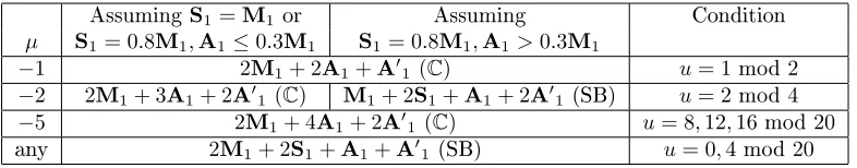
3.5.2 Summary of choices and complexities forFp2 arithmetic
We saw that we trivially haveA2 = 2A1 andA02= 2A01 whatever the choice
made to build Fp2. The situation is more complicated for M2 and S2; it is
summarized in Tables 1 and 2. In these tables SB, K andCdenote the method
used.
µ AssumingA1≤0.33M1 AssumingA1>0.33M1 Condition
−1 3M1+ 5A1 (K) 4M1+ 2A1(SB) u= 1mod2
−2 3M1+ 5A1+A01 (K) 4M1+ 2A1+A01(SB) u= 2mod4
−5 3M1+ 6A1+ 2A01(K) 4M1+ 3A1+ 2A01 (SB) u= 8,12,16mod20
any 4M1+ 5A1 (K) 5M1+ 2A1(SB) u= 0,4mod20
Table 1: Complexities ofM2 depending on the way to buildFp2
AssumingS1=M1 or Assuming Condition
µ S1= 0.8M1,A1≤0.3M1 S1= 0.8M1,A1>0.3M1
−1 2M1+ 2A1+A01(C) u= 1 mod2
−2 2M1+ 3A1+ 2A01 (C) M1+ 2S1+A1+ 2A01 (SB) u= 2 mod4
−5 2M1+ 4A1+ 2A01(C) u= 8,12,16mod20
any 2M1+ 2S1+A1+A01 (SB) u= 0,4mod20
Table 2: Complexities ofS2depending on the way to buildFp2
Remark 4. The inuence of the relative cost of A01 compared to A1 is small
and even negligible, even if−2 is chosen to deneFp2
Thanks to Tables 1 and 2, it is easy to choose the best algorithm for Fp2
multiplication and squaring depending on the context (relative cost ofFp
3.6 Choice of
F
p12arithmetic in the case
2
,
3
,
2
We assume thatFp12 is built over Fp2 viaFp6, using someξ which is neither a
square nor a cube inFp2:
Fp6 =Fp2[β]whereβ3=ξandFp12 =Fp6[γ]withγ2=β.
3.6.1 Fp6 arithmetic
We saw in Section 3.3.2 that the Karatsuba method becomes interesting when
M2≥3A2. Regarding Table 1, this condition is clearly always satised.
There-fore, the Karatsuba method should always be used forFp6/Fp2 multiplications
and
M6= 6M2+ 15A2+ 2m2,ξ.
It is also easy to study the dierence between the complexities of the schoolbook, the Karastuba and the Chung-Hasan methods and to conclude that the latter is better in each case of Tables 1 and 2. Therefore, the Chung-Hasan method should always be use forFp6/Fp2 squaring so
S6= 2M2+ 3S2+ 8A2+A02+ 2m2,ξ.
3.6.2 Fp12 arithmetic
We obviously haveA12= 2A6= 12A1andA012= 2A06= 12A01.
Fp12 multiplication. According to Section 3.2, the Karatsuba method is
bet-ter than the schoolbook method when 3A6 < M6, which is obviously always
the case according to 3.6.1. TheFp6 multiplication byβ involved in Karatsuba
formulas is given by
b0+b1β+b2β2
β =ξb2+b0β+b1β2,
thusm6,β = m2,ξ. Finally, the Karatsuba method should always be used for
Fp12/Fp6 multiplications and
M12= 18M2+ 60A2+ 7m2,ξ.
Fp12 sparse multiplication. During the Miller loop for the optimal Ate
pair-ing, one of the operands (the line`) is sparse but the conclusion remains the
same: the Karatsuba method should be preferred for multiplications at all lev-els, assuming that at least two coecients are non-zero. More precisely, as explained in Section 6,`is of the formb0+b1γ+b3γ3, wherebi∈Fp2. With our
notations, it can be written`=b0+ (b1+b3β)γ. The Karatsuba multiplication
inFp12 between`andc0+c1γis given by
b0c0+ (b1+b3β)c1β+ ((b0+b1+b3β) (c0+c1)−b0c0−(b1+b3β)c1) (1)
• one multiplication ofc0∈Fp6 byb0∈Fp2 which trivially costs3M2,
• one multiplication ofc1∈Fp6 byb1+b3β. It is done thanks to the sparse
Karatsuba multiplication given in Section 3.3 and costs5M2+6A2+m2,ξ,
• 4A2 to computeb0+b1and c0+c1,
• one multiplication ofc0+c1 byb0+b1+b3β which is the same as the one
ofc1 byb1+b3β,
• onem6,β=m2,ξ and3A6 to compute the nal result.
Hence aFp12 sparse multiplication requires
sM12= 13M2+ 25A2+ 3m2,ξ.
Fp12 squaring. Let us now compare the schoolbook and the Karatsuba
meth-ods for squaring inFp12/Fp6. Using the complexities obtained forM6 and S6
in 3.6.1, the dierence between the complexities is
SK
12−S
SB
12= 3S2−4M2+ 2A2−2A02+m2,ξ.
Using Tables 1 and 2, we can easily verify that this dierence is negative in all the cases we have considered even ifm2,ξ =M2 (which is obviously the worst
case form2,ξ). Therefore, the schoolbook method should not be used.
We have now to compare the Karatsuba and the complex methods for squar-ing in Fp12/Fp6. Using the complexities obtained for M6 and S6 in 3.6.1 and
assuming that m6,β+1 =A6+m6,β =A6+m2,ξ, the dierence between the
complexities is
∆ =SK
12−SC12= 9S2−6M2−6A2+m2,ξ
The sign of∆depends on the value ofµ. Again, we do not give all the details
but thanks to Tables 1 and 2, we can determine that
• The Karatsuba method should be used ifµ=−1,−5and ifµ=−2with
A1≤0.33M1or S1= 0.8M1 and in this case
S12= 6M2+ 9S2+ 36A2+ 3A02+ 7m2,ξ.
• The complex method should be used ifµis not small and ifµ=−2with
A1>0.33M1andS1=M1and in this case
S12= 12M2+ 42A2+ 3A02+ 6m2,ξ.
3.7 Choice of
F
p12arithmetic in the case
2
,
2
,
3
We assume thatFp12 is built over Fp2 viaFp4, using someξ which is neither a
square nor a cube inFp2:
3.7.1 Fp4 arithmetic
We saw in Section 3.2.2 that the Karatsuba method becomes interesting when
M2≥3A2= 6A1. Regarding Table 1, this condition is clearly always satised.
Therefore, the Karatsuba method should always be used for Fp4/Fp2
multi-plications and
M4= 3M2+ 5A2+m2,ξ.
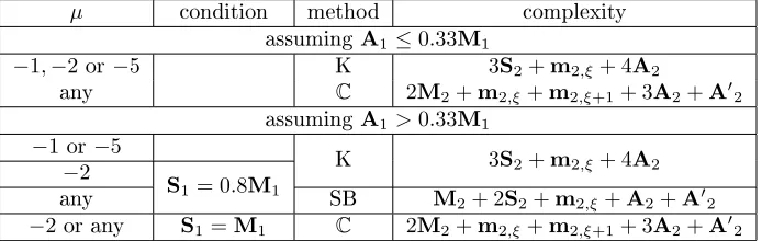
Concerning the squaring, all the methods are close in terms of complexity. We do not give details here, but thanks to Tables 1 and 2, we can decide which method is preferable to use, depending on the context. The Karatsuba method is usually the best and this is summarized in Table 3.
µ condition method complexity
assumingA1≤0.33M1
−1,−2or −5 K 3S2+m2,ξ+ 4A2
any C 2M2+m2,ξ+m2,ξ+1+ 3A2+A02
assumingA1>0.33M1
−1 or−5
K 3S2+m2,ξ+ 4A2
−2
S1= 0.8M1
any SB M2+ 2S2+m2,ξ+A2+A02
−2or any S1=M1 C 2M2+m2,ξ+m2,ξ+1+ 3A2+A02
Table 3: Complexities ofS4 depending on the context
3.7.2 Fp12 arithmetic
We also haveA12= 12A1 andA01212A01 in this case.
Fp12 multiplication. According to Section 3.3, the Karatsuba method is
bet-ter than the schoolbook method for multiplications inFp12/Fp4when3A4<M4,
which is obviously always the case according to Section 3.7.1. TheFp4
multi-plication byβ involved in Karatsuba formulas is given by
(b0+b1β)β =ξb1+b0β,
thusm4,β =m2,ξ. Therefore, the Karatsuba method should always be used for
Fp12/Fp4 multiplications and
M12= 18M2+ 60A2+ 8m2,ξ.
Fp12 sparse multiplication. Again, the Karatsuba method should be
`=b0+b3β+b1γ. We use the sparse Karatsuba multiplication given in Section
3.3 to compute the product of` andc0+c1γ+c2γ2∈Fp12
(c0+c1γ+c2γ2)((b0+b3β) +b1γ) =c0(b0+b3β) +βc2b1
+ [(c0+c1)(b0+b3β+b1)−c0(b0+b3β)−c1b1]γ
+ [c2(b0+b3β) +c1b1]γ2 (2)
It requires
• Two multiplications of c1 (or c2)∈ Fp4 by b1 ∈Fp2 which trivially cost
2M2each.
• ThreeFp4 multiplications which are done thanks to the Karatsuba method
and cost3M2+ 5A2+m2,ξ.
• 3A2 to computeb0+b1and c0+c1.
• Onem4,β =m2,ξ and4A4 to compute the nal result.
Hence aFp12 sparse multiplication requires
sM12= 13M2+ 26A2+ 4m2,ξ.
Fp12 squaring. We do not give details here because it would be repetitive after
previous sections but it is easy to study the dierence between the complexi-ties of the schoolbook, the Karastuba and the Chung-Hasan methods and to conclude that the latter is always better. Therefore, the Chung-Hasan method should always be used forFp12/Fp4 squaring and
S12= 3S4+ 6M2+ 26A2+ 2A02+ 4m2,ξ.
3.8 Choice of
ξ
and consequences on
u
The choice of ξ has no consequence on the way of choosing the arithmetic of
Fp12, but it must be done such that multiplication byξis as ecient as possible.
However, the choice ofξ has less inuence on M12 and S12 complexities than
the choice ofµ. So an ecientµshould be chosen in priority.
The most natural choice isξ=α, so that a multiplication byξ inFp2 is
(a0+a1α)ξ=µa1+a0α
and thus m2,ξ =m1,µ. It means that µ must be neither a fourth power nor a
cube inFp. If p≡1 (mod 6), which is always the case for a BN prime, such a
µalways exists.
In practice, it is easy to nd one by trial and error, by factoringx12−µ
not necessarily optimal for Fp2 arithmetic and µ should be chosen in priority
to deneFp2 as eciently as possible. For example, the best choice for Fp2 is
µ=−1 but it is obviously always a cube. Then, ifµ is already xed to dene
Fp2 and is a cube,ξmust be chosen as an element ofFp2 with small coecients.
At rst glance, the best choices areξ= 2andξ= 1 +α. However, as proved in
Corollary 1 of Appendix A,2(as any other element ofFp) is always a square in
Fp2, so it cannot be chosen to deneFp12. Other choices can be made as2 +α
but they are of course less interesting in terms of eciency.
Remark 5. The condition to chooseξis that it is neither a square nor a cube
in Fp2. Since −1 is always a square and a cube in Fp2, there is no interest to
consider the sign of ξ. In the same way, there is no interest to consider the
conjugates ofξbecause they are squares and cubes at the same times as ξ.
Let us now precise the possible choices forξdepending on the choice ofµand
their consequences on the choice of the parameteru. We will use the following
proposition which is proved in Appendix A:
Proposition 3. Let p be an odd prime number which is equal to 1 modulo 3 (this is always the case for BN primes). Then an element is a square (resp. a cube) inFp2 if and only if its norm is a square (resp. a cube) inFp.
3.8.1 The case µ=−1
In this case, the smallest complexity form2,ξ is reached byξ= 1 +iand equals
2A1 since
(1 +i)(a0+a1i) =a0−a1+ (a0+a1)i.
Let us now study the conditions onuensuring that1 +iis neither a square nor
a cube inFp2.
Theorem 1. Letp= 36u4+ 36u3+ 24u2+ 6u+ 1 be a BN prime withuodd
(thusFp2 can be dened byi= √
−1). Then1 +iis neither a square nor a cube
in Fp2 if and only if u= 7 or 11 modulo 12. In this case,Fp12 can be dened
overFp2 by a sixth root of1 +i.
Proof. By Proposition 3,1 +iis a square (resp. a cube) in Fp2 if and only if
2 =NF
p2/Fp(1 +i)is a square (resp. a cube) inFp.
• According to Proposition 1 of Appendix A,2is a square inFpif and only
ifu= 0or1modulo4. Thus, in our situation,1 +iis not a square inFp2
if and only ifu= 3modulo4.
• In the same way,1 +iis not a cube if and only if2 is not a cube which means, according to Proposition 2 of Appendix A, that u 6= 0 mod 3. Thus1 +iis not a cube if and only ifu= 1or5 modulo6.
If1+icannot be chosen,ξshould be sought in the forma+ibwitha > b >0 and can be chosen if and only ifa2+b2=NF
p2/Fp(a+ib)is neither a square nor
a cube in Fp. The next candidate in terms of eciency isξ= 2 +ifor which
m2,ξ = 2A1+ 2A01 and whose norm is 5. Combining the condition ensuring
that 5 is neither a square nor a cube given in Appendix A and the fact that
u6= 7 or 11modulo12 (otherwise ξ= 1 +i can be chosen), we get that2 +i
should be chosen to dene Fp12 if u = 1,3,13,27,33,37,41 or 57 modulo 60
but not in the12remaining cases (u= 5,9,15,17,21,25,29,39,45,49,51or53 modulo60). In 3of these cases (u= 17,39and53modulo60), one can choose 3 +i, whose norm is 10. Of course, this study can be easily continued with "larger" values of ξ (4 +i,3 + 2i, ...) to be able to deal with the 9 remaining cases. But the interest is limited here and the reader can easily do it by himself if necessary.
3.8.2 The case µ=−2
Taking in account the results from Section 3.5, this choice should be made only when−1cannot be chosen to buildFp2, that is, when u= 2modulo4(−1is a
square and−2is not a square). In this case, the smallest complexity form2,ξis
reached byξ=α=√−2. Let us now study the conditions onuensuring that
√
−2is neither a square nor a cube inFp2.
Theorem 2. Letp= 36u4+ 36u3+ 24u2+ 6u+ 1be a BN prime withu= 2 modulo4 (thusFp2 can be dened by
√
−2but not by √−1). Thenα=√−2 is neither a square nor a cube inFp2 if and only ifu= 2or10modulo 12. In this
case,Fp12 can be dened overFp2 by a sixth root ofα.
Proof.
• Since −1 is a square and −2 is not, NF
p2/Fp(α) = 2 is never a square in
Fp and thus, by 3,αis never a square inFp2. Note that this proof is not
specic to the case µ=−2; it is only using the fact that−1 is a square inFpand µis not.
• Since −1 is a cube, αis a cube in Fp2 if and only if2 = −NF
p2/Fp(α)is
a cube inFp. According to Proposition 2 of Appendix A, 2, and thusα,
is not a cube if and only ifu= 1or 2 modulo3. Taking in account that
−1is a square and−2is not a square, this last condition can be rewritten
u= 2or10modulo12.
The next interesting candidate is ξ = 1 +α but it cannot be chosen since
its norm equals3 which is always a square inFp in the remaining case (u= 6
modulo12). The situation is better ifξ= 2 +αwhose norm is6. Indeed, since 2is not a square and3is always a square,6is never a square in Fp. Moreover,
since it was not possible to chooseξ=α,2 is a cube inFp and thus6 is not a
Appendix A,ξ= 2 +αcan then be chosen ifu= 6or30modulo36. In this case
m2,ξ= 2A1+ 2A01. Again, this study can be easily continued by the interested
reader with "larger" values ofξ like3 +αto deal with the last remaining case
(u= 18modulo36).
3.8.3 The case µ=−5
Again, taking in account the results from Section 3.5, this case should be con-sidered only ifu= 8,12or16modulo20(−1,±2are squares and ±5 are not). The smallest complexity form2,ξis reached byξ=α=
√
−5. Let us study the conditions onuensuring that √−5is neither a square nor a cube inFp2.
Theorem 3. Letp= 36u4+ 36u3+ 24u2+ 6u+ 1be a BN prime withu= 8,12
or16 modulo 20. Then α=√−5 is neither a square nor a cube in Fp2 if and
only ifu= 12,16,28,48,52,56modulo60. In this case, Fp12 can be dened over
Fp2 by a sixth root ofα.
Proof. Similarly to the proof of Theorem 2, we prove thatαis never a square
in Fp2. Moreover,α is a cube inFp2 if and only if 5 =−NF
p2/Fp(α)is a cube
inFp. Proposition 2 of Appendix A gives a condition ensuring that5, and thus
α, is not a cube and allows to conclude.
The next interesting candidate is ξ = 1 +α but it cannot be chosen since
its norm equals6 which is always a square in this case. The situation is the same for2 +αsince its norm is9. The "smallest" usable candidates are1 + 2α
and 3 +α whose norms are respectively21 and 14. This will give conditions onumodulo7but we leave it to the interested reader, since there are very few concerned cases (u= 8,32or36modulo60) and the cost ofm2,ξ becomes high.
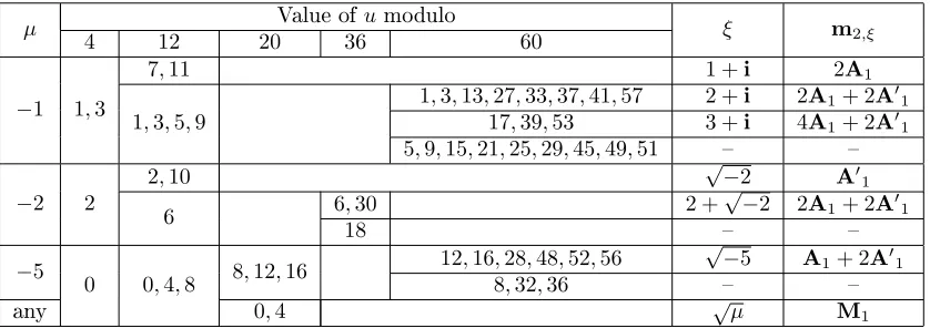
3.8.4 Recapitulative table
Finally, we gave almost all the best choices forξ, depending on the value of u.
This is summarized in Table 4.
µ Value ofumodulo ξ m2,ξ
4 12 20 36 60
−1 1,3
7,11 1 +i 2A1
1,3,5,9
1,3,13,27,33,37,41,57 2 +i 2A1+ 2A01
17,39,53 3 +i 4A1+ 2A01
5,9,15,21,25,29,45,49,51
−2 2
2,10 √−2 A01
6 6,30 2 +
√
−2 2A1+ 2A01
18
−5
0 0,4,8 8,12,16
12,16,28,48,52,56 √−5 A1+ 2A01
8,32,36
any 0,4 õ M1
3.9 New improvements of
F
p12arithmetic
Usually, the cost of additions is not taken in account in complexity studies because it is assumed to be negligible. However, it is not always the case in hardware or assembly language where the ratio between additions and multi-plications in Fp can be as large as 0.2 to 0.5, as explained in Section 3.1. In
this case, we get some new improvements (saving of course only additions). The rst one is just a computational trick and is probably used in practical imple-mentations but it is usually not explicitly written. The second one consists in precomputing the traces of some elements of the intermediate levels of the ex-tension tower which are involved in several operations.
Since these are new results, we chose to present them in a dedicated section. These results could be included in our previous discussion on the choices for building Fp12. We did not do it for two reasons. The rst one is that they
require some precomputations storage which is not always desirable, depending on the context. The second one is that it has no inuence on the choices to be made.
3.9.1 Multiplications byξ−1 in Karatsuba operations
Ifmi,ξ−1≤mi,ξ, then the Karatsuba multiplication ofx0+x1β byy0+y1β in
Fp2i can be evaluated as
x0y0+x1y1+ (ξ−1)x1y1+ ((x0+x1)(y0+y1)−x0y0−x1y1)β,
instead of
x0y0+ξx1y1+ ((x0+x1)(y0+y1)−x0y0−x1y1)β.
Then it requires 3Mi +mi,ξ−1+ 5Ai instead of 3Mi+mi,ξ + 5Ai because
x0y0+x1y1is used twice.
In the same way, the Karatsuba multiplication of x0+x1β +x2β2 by y0 +
y1β+y0β2 in Fp3i can be evaluated as
x0y0+ξ((x1+x2)(y1+y2)−x1y1−x2y2)
+ [(x0+x1)(y0+y1)−x0y0−x1y1+x2y2+ (ξ−1)x2y2]β
+ [(x0+x2)(y0+y2)−x0y0−(−x1y1+x2y2)]β2.
One of the multiplications by ξ is then replaced by a multiplication by ξ−1 compared to the formula given in 3.3.2. Of course, both in the case of quadratic and cubic extensions, this trick also applies to Karatsuba squaring.
In the cases considered in Section 3.8, this improvement is only interesting in the intermediate elds (Fp4/Fp2 in the2,2,3 case and Fp6/Fp2 in the 2,3,2
case) and allows to save someFpadditions for each Karatsuba multiplication or
ξ m2,ξ−1 m2,ξ Saving
1 +i 0 2A1 2A1
2 +i 2A1 2A1+ 2A01 2A01
3 +i 2A1+ 2A01 4A1+ 2A01 2A1
2 +√−2 2A1+A01 2A1+ 2A01 A01
Table 5: Savings provided by theξ−1trick
Remark 6. This trick is more interesting in the case 2,2,3 that in the case 2,3,2. Indeed, a Karatsuba multiplication in Fp12 requires6 multiplications at
the middle level in the case2,2,3 (and then6m2,ξ are replaced by6m2,ξ−1) but
only 3 in the case 2,3,2. Of course, this remark also applies to sparse Fp12
multiplications and toFp12 squarings.
3.9.2 Precomputed traces
In the case where memory is large enough, we can perform some pre-computations to speed up the dierent operations (i.e.MiorSi). In particular, it could be
in-teresting to precompute the trace of an element if this element is used in several operations (requiring its trace) in the following.
For example, assuming thatx0+x1=trFp2i/Fpi(x0+x1α)is precomputed,
computing(x0+x1α)2 inFp2i using the Karatsuba method as in 3.2.3 requires
only3Si+mi,µ+ 3Ai instead of3Si+mi,µ+ 4Ai. The same remark holds for
all the methods for squaring or multiplying inFp2i orFp3i involving traces (or
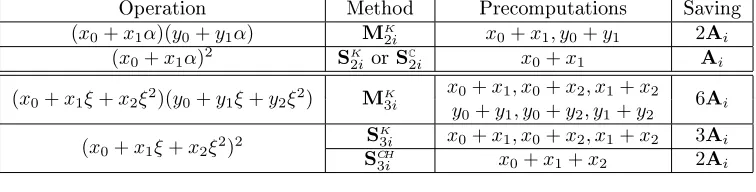
more precisely sums of coordinates). It is summarized in Table 6 (notations are those of Sections 3.2 and 3.3).
Operation Method Precomputations Saving (x0+x1α)(y0+y1α) MK2i x0+x1, y0+y1 2Ai
(x0+x1α)2 SK2i or SC2i x0+x1 Ai
(x0+x1ξ+x2ξ2)(y0+y1ξ+y2ξ2) MK3i
x0+x1, x0+x2, x1+x2
6Ai
y0+y1, y0+y2, y1+y2
(x0+x1ξ+x2ξ2)2
SK
3i x0+x1, x0+x2, x1+x2 3Ai
SCH
3i x0+x1+x2 2Ai
Table 6: Precomputing traces
Of course, we get savings only if the precomputations are used in several opera-tions. This may hold in the arithmetic of the extension tower when an element is used twice. For example, a schoolbook multiplication inFp2i will usex0both
forx0y0and forx0y1. If these multiplications are performed with the Karatsuba
method in Fpi, precomputing the trace of x0 is interesting because it is used
twice. However, in Karatsuba operations or in complex squarings, no element is used twice. As a consequence, this is not interesting for multiplications inFp12
when the Chung-Hasan method is used over Karatsuba or complex arithmetic. It can also be applied for sparse multiplications since it involves schoolbook steps if operands have only one non-zero coecient. Finally, we can also pre-compute traces if oneFp12 element is used for several multiplications, which is
usually the case in the nal exponentiation step. Let us now give more details about these three situations.
3.9.3 Use of precomputed traces inFp12 squarings
Some coecients are used several times in Fp12 squaring if the Chung-Hasan
method is used over Karatsuba or complex arithmetic (i.e. whenA1is not very
expensive compared to M1). Indeed, we know from Section 3.3 that x0,2x1
andx2 are used twice to compute(x0+x1α+x2α2)2 using the Chung-Hasan
method in Fp3i/Fpi. Thus3Ai can be saved in SCH3i if traces are precomputed
at the leveli. We saw in Sections 3.6 and 3.7 that this method is always used
but one can do even better, depending on the way to buildFp12.
Case 2,3,2. We saw in Section 3.6 that the Karatsuba method is usually used for the Fp12/Fp6 squaring, so that the Chung-Hasan squaring inFp6 is used 3
times to compute(c0+c1γ)2 (forc02, c21 and(c0+c1)2). Of course each of them
is used only once but precomputing traces is nonetheless interesting because
trF
p6/Fp2(c0+c1) = trFp6/Fp2(c0) +trFp6/Fp2(c1) which requires only one A2
instead of 2 if it is computed directly. Hence, in this case, if the Karatsuba method is used inFp2,11A1can be saved inS12thanks to trace precomputations
(9 from Fp6/Fp2 Chung-Hasan over Karatsuba squaring and 2 from Fp12/Fp6
Karatsuba over Chung-Hasan squaring). If the Karatsuba method is not used inFp2, which means thatA1>0.33M1, only2A1 can be saved (fromFp12/Fp6
Karatsuba over Chung-Hasan squaring).
Case 2,2,3. We saw that when we compute(c0+c1γ+c2γ2)2with the
Chung-Hasan method c0, c1 and c2 ∈ Fp4 are used twice. For example c0 is used in
c2
0 and in 2c0c1, so that precomputing t0 =trFp4/Fp2(c0) saves one A2. But,
assuming thatc0=b0+b1β,b0∈Fp2 is also used twice (also inc20 and in2c0c1
whatever the methods used) and precomputing its trace is then interesting if the Karatsuba/complex method is used in Fp2. Moreover for Fp4 Karatsuba
or complex operations, t0 plays the same role as b0 so that precomputing its
trace is also interesting. Finally, in this case and if the Karatsuba method is used inFp2,15A1can be saved inS12 thanks to trace precomputations (6from
theFp4/Fp2 traces of the ci, 6 from the Fp2/Fp traces of the Fp2 components
of the ci and3 from the Fp2/Fp traces of theFp4/Fp2 traces of the ci). If the
Karatsuba method is not used in Fp2, which means that A1 >0.33M1, only
3.9.4 Use of precomputed traces inFp12 sparse multiplications
The sparse multiplication involved in the Miller loop for the optimal Ate pairing involves schoolbook steps if operands have only one non-zero coecient. Again, the savings are depending on the way to buildFp12
Case 2,3,2. Looking at formula (1) given in Section 3.6.2, we can see that
• b0is used in3Fp2 multiplications. Precomputing its trace then saves2A1,
• b1 and the third component ofc1are used in2Fp2 multiplications during
the sparse product(b1+b3β)c1, so 2A1 can be saved,
• The same holds for the sparse product(b0+b1+b3β)(c0+c1),
• b3 is used twice in each of these sparse products, so3A1can be saved by
precomputingtrF
p2/Fp(b3).
Finally,9A1can be saved in the sparse multiplication if traces are precomputed
(assuming that the Karatsuba method is used forFp2 multiplications, i.e. that
A1≤0.33M1)
Case 2,2,3. Looking at formula (2) given in Section 3.7.2, we can see that
• b0+b3β is used in2Fp4 multiplication. Precomputing its trace (b0+b3)
savesA2,
• As a consequence of the previous point, b0, b3 and b0+b3 are used in 2
Fp2 multiplications, so3A1can be saved,
• b3is also used in theFp4 product(c0+c1)(b0+b1+b3β)so one additional
A1 can be saved,
• b1 is used in4Fp2 multiplications (c2b1andc1b1) so3A1can be saved by
precomputingtrF
p2/Fp(b1),
• c2is used twice (inc2b1and inc2(b0+b3β)) so itsFp2 coecients are used
twice each which saves2A1.
Finally, 11A1 can be saved in the sparse multiplication if traces are
precom-puted (assuming that the Karatsuba method is used for Fp2 multiplications,
i.e. thatA1≤0.33M1, otherwise only2A1are saved).
In all considered cases, the saving obtained is around 10% of the total num-ber of additions inFp12 operations which is not negligible if the relative cost of
3.9.5 Use of precomputed traces in the nal exponentiation
Full multiplications in Fp12 are only used in the nal exponentiation (in the
Miller loop, sparse multiplications are used). If the implemented exponentiation parses the exponent from left to right (which is usually the case), then the multiplication steps are performed with one constant term c. Hence, we can
precompute and store all the traces depending only onc. Since the Karatsuba
method is used at all levels of the extension tower (except in Fp2 if A1 >
0.33M1), we will signicantly reduce the number of required additions, whatever
the way to buildFp12.
Case 2,3,2.
• MK
12 requires the Fp12/Fp6 trace of c, thus one A6 can be saved if this
trace is already precomputed. It also requires 3MK
6 with one constant
term (the2 coordinates ofc and its trace).
• EachMK
6 involving a constant termb requires3sums of2 coordinates of
b, thus 3A2 can be saved if these sums are precomputed. Hence 9A2 are
saved at this level. Each MK
6 also requires6M2 with one constant term
(the3coordinates ofb and the3sums of2coordinates).
• EachMK
2 involving a constant termarequires theFp2/Fptrace ofa, thus
one A1 can be saved if this trace is precomputed. Hence 18A1 can be
saved at this level when the Karatsuba method is used for M2 (i.e. if
A1≤0.33M1according to Section 3.5).
Case 2,2,3.
• MK
12 requires3sums of2coordinates ofc, thus3A4can be saved if these
sums are precomputed. It also requires6MK
4 with one constant term (the
3coordinates of cand the3 sums of2 coordinates).
• EachMK
4 involving a constant termbrequires theFp4/Fp2 trace ofb, thus
one A2 can be saved if this trace is precomputed. Hence 6A2 are saved
at this level. EachMK
4 also requires3M2 with one constant term (the 2
coordinates ofb and its trace).
• Again, one A1 can be saved for each MK2 involving a constant term if
its trace is precomputed. Hence 18A1 can be saved at this level when
the Karatsuba method is used forM2 (i.e. if A1≤0.33M1 according to
Section 3.5).
In both cases, 42A1 can be saved for each multiplication in Fp12 involving
a constant term if its traces are precomputed. This is about20% of the total number of additions inM12which is signicant if the relative cost of an addition
compared to a multiplication inFpis not small. IfA1>0.33M1, the schoolbook
3.10 Summary of
F
p12arithmetic
In the previous sections, we explained how to choose the tower eld depending onuand on the relative cost ofFp operations. We also saw that the arithmetic
choices to be made are essentially depending on theFp2 arithmetic. Let us now
recapitulate these choices.
3.10.1 The caseµ=−1
This choice can be made ifuis odd andξcan be chosen "small" in most cases :
• ξ= 1 +iifu= 7or 11modulo12andm2,ξ = 2A1,
• ξ= 2+iifu= 1,3,13,27,33,37,41,57modulo60andm2,ξ= 2A1+2A01,
• ξ= 3 +iifu= 17,39or 53modulo60andm2,ξ = 4A1+ 2A01.
Let us rst assume thatA1≤0.33M1. In this case, the fullFp12 multiplication
and the sparse multiplication should be done using Karatsuba arithmetic at all levels of the tower. Concerning the Fp12 squaring, the Chung Hasan method
should be used for squaring in the degree 3 extension (Fp6/Fp2 or Fp12/Fp4)
but all the other multiplications should use the Karatsuba method. The overall complexities are summarized in Table 7. For the complexities using our new improvements given in Section 3.9, we assumed that M12 is only used in the
nal exponentiation andsM12 is only used in the Miller loop (which is always
the case in practice). We also assumed for simplifying that theξ−1trick saves 2A1 whatever the choice ofξ(in fact it saves2A01 instead of2A1 ifξ= 2 +i).
An interesting point is that, if our improvements are used, the results given in Table 7 also hold ifA1>0.33M1 (because less additions are required). Finally,
in this table (as well as in the following ones), K, CH, SB and C denote the
methods used for arithmetic and SB/C means that the schoolbook method is
used for multiplications and the complex method is used for squarings.
Oper- Case Arithmetic used Number of operations
ation without/with improvement
Fp2 Fp4 Fp6 Fp12 M1 A1 A01 m2,ξ
M12
2,3,2
K K K 54 210/162 0 7
2,2,3 K 210/156 8
sM12
2,3,2
K K K 39 115/106 0 3
2,2,3 K 117/100 4
S12
2,3,2
K/C CH K 36 120/109 15 7
2,2,3 K CH 124/99 13
Table 7: Fp12 complexities if µ = −1 (assuming A1 ≤ 0.33M1 if our new
improvements are not used)
the art (see [20, 14, 3, 27] for example). However, our improvements take more advantage of a 2,2,3 extension tower and then this way to build Fp12 becomes
the one to choose.
The other cases are quite similar so we are only giving the nal complexities in tables. Let us rst give in Table 8 theFp12 complexities ifA1>0.33M1.
Oper- Case Arithmetic used Number of operations ation Fp2 Fp4 Fp6 Fp12 M1 A1 A01 m2,ξ
M12
2,3,2
SB K K 72 156 0 7
2,2,3 K 156 8
sM12
2,3,2
SB K K 52 76 0 3
2,2,3 K 78 4
S12
2,3,2
SB/C CH K 42 102 15 7
2,2,3 K CH 106 13
Table 8: Fp12 complexities if µ=−1 assuming our improvements are not used
andA1>0.33M1
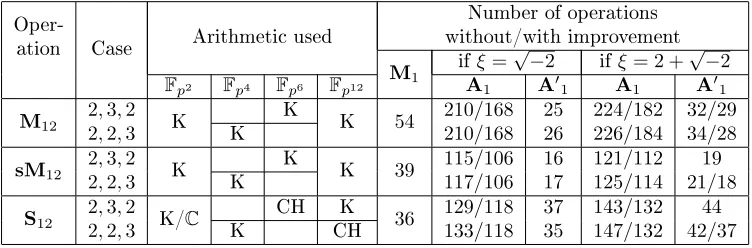
3.10.2 The caseµ=−2
This choice should be made if the previous one cannot, in the case whereu= 2 modulo4. Tables 9 and 10 give the complexities of Fp12 operations when ξ = √
−2(which means, according to Section 3.8, thatu= 2or10modulo12) and whenξ= 2 +√−2(which means thatu= 6 or30modulo36but not18).
Oper-Case Arithmetic used
Number of operations
ation without/with improvement
M1 if
ξ=√−2 ifξ= 2 +√−2
Fp2 Fp4 Fp6 Fp12 A1 A01 A1 A01
M12
2,3,2
K K K 54 210/168 25 224/182 32/29 2,2,3 K 210/168 26 226/184 34/28
sM12
2,3,2
K K K 39 115/106 16 121/112 19 2,2,3 K 117/106 17 125/114 21/18
S12
2,3,2
K/C CH K 36 129/118 37 143/132 44
2,2,3 K CH 133/118 35 147/132 42/37
Table 9: Fp12 complexities if µ=−2 (assumingA1 ≤0.33M1 if our
Oper- Case Arithmetic used Number of operations
ation M1 if
ξ=√−2 ifξ= 2 +√−2
Fp2 Fp4 Fp6 Fp12 A1 A01 A1 A01
M12
2,3,2
SB K K 72 156 25 170 32
2,2,3 K 156 26 172 34
sM12
2,3,2
SB K K 52 76 16 82 19
2,2,3 K 78 17 86 21
S12 2,3,2 SB K C 48 108 24 120 30
S1 =M1 2,2,3 K/C CH 106 32 126 42
S12 2,3,2 SB CH K 47.4 93 37 107 44
S1 =0.8M1 2,2,3 K CH 97 35 111 40
Table 10: Fp12 complexities ifµ=−2assuming our improvements are not used
andA1>0.33M1
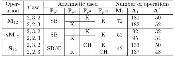
3.10.3 The caseµ=−5
This choice should be made if the previous ones cannot, in the case whereu= 8,12or16modulo20. Tables 11 and 12 give the complexities ofFp12operations
whenξ=√−5which means, according to Section 3.8, thatu= 12,16,28,48,52 or56modulo60(but not8,32or36).
Oper- Case Arithmetic used Number of operations
ation without/with improvement
Fp2 Fp4 Fp6 Fp12 M1 A1 A01
M12
2,3,2
K K K 54 225/183 50
2,2,3 K 226/184 52
sM12
2,3,2
K K K 39 131/122 32
2,2,3 K 134/123 34
S12
2,3,2
K/C CH K 36 151/140 50
2,2,3 K CH 155/140 48
Table 11: Fp12 complexities ifµ=−5 (assumingA1≤0.33M1 if our
improve-ments are not used)
Oper- Case Arithmetic used Number of operations ation Fp2 Fp4 Fp6 Fp12 M1 A1 A01
M12
2,3,2
SB K K 72 181 50
2,2,3 K 182 52
sM12
2,3,2
SB K K 52 92 32
2,2,3 K 95 34
S12
2,3,2
SB/C CH K 42 133 50
2,2,3 K CH 137 48
Table 12: Fp12 complexities ifµ=−5assuming our improvements are not used
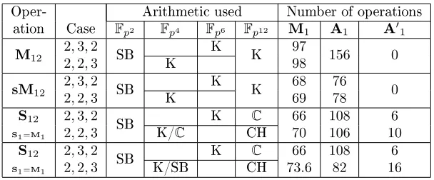
3.10.4 The caseµ large
This choice should be made if u = 0 or 4 modulo 20 and we assume that
ξ = √µ since it is always possible to choose such a µ. In this case, we have m1,µ=m2,ξ=M1 and the complexities ofFp12 operations are given in Tables
13 and 14.
Oper- Case Arithmetic used Number of operations
ation without/with improvement
Fp2 Fp4 Fp6 Fp12 M1 A1 A01
M12
2,3,2
K K K 79 210/168 0
2,2,3 K 80 210/168
sM12
2,3,2
K K K 55 115/106 0
2,2,3 K 56 117/106
S12
2,3,2
K K C 54 144/133 6
2,2,3 K/C CH 58 142/127 10
Table 13: Fp12 complexities ifµis large (assumingA1≤0.33M1if our
improve-ments are not used)
Oper-Case Arithmetic used Number of operations ation Fp2 Fp4 Fp6 Fp12 M1 A1 A01
M12
2,3,2
SB K K 97 156 0
2,2,3 K 98
sM12
2,3,2
SB K K 68 76 0
2,2,3 K 69 78
S12 2,3,2 SB K C 66 108 6
S1 =M1 2,2,3 K/C CH 70 106 10
S12 2,3,2 SB K C 66 108 6
S1 =M1 2,2,3 K/SB CH 73.6 82 16
Table 14: Fp12 complexities if µ is large assuming our improvements are not
used andA1>0.33M1
3.10.5 Some remarks
Looking at these tables, we can make some interesting remarks:
• As noticed in Remark 7 buildingFp12 with a2,3,2 tower remains
prefer-able in most cases to a2,2,3tower if our new improvements are not used but this is no longer the case if there are used. Anyway, the dierence between the complexities of the two choices for buildingFp12 is negligible.
• As already mentioned, the choice ofµhas a great inuence on the number
of additions involved inFp12 arithmetic, so it should be chosen rst, even
if the choice of ξis not optimal in this case. For example, it is better to
• Our new improvements have a signicant impact on Fp12 arithmetic if
Fp additions are costly which, as explained in Section 3.1, is often the
case in low level implementations. For example if A1 = 0.25M1 (which
is probably not far from the average cost of additions in hardware im-plementations), our improvements are providing a gain between 6 and 13% on Fp12 arithmetic (and then on pairing computation). In fact the
gain is even not so negligible if Fp additions are cheap (like in software
implementations). For example, ifA1= 0.1M1, it is between3and7%.
• The cost ofFp squaring (with respect to Fp multiplication) and Fp
dou-bling (with respect to Fp addition) have very few impact on the choices
to be made forFp12 arithmetic.
4 Choosing
u
The parameteruis involved at several levels of the pairing computation, so that
the best choice is not trivial to do. Let us summarize the constraints onuthat
we have to deal with in order to make a good choice.
• The parameteruis dening the security level. Indeed, it is both
parametriz-ing the size of the elliptic curve (whose prime order is36u4+ 36u3+ 18u2+
6u+ 1) and the number of elements of the target nite eld (which is (36u4+ 36u3+ 24u2+ 6u+ 1)12).
• It is involved as an exponent in the Miller loop. More precisely, in the case
of an optimal Ate pairing, the exponent of the Miller loop is 6u+ 2. In order to optimize this step,ushould be chosen such that6u+ 2is sparse.
• It is involved as an exponent in the nal exponentiation. If the addition
chain given in Section 2.4 is used, u is directly used (three times) as
an exponent, so it should be sparse to ensure a fast nal exponentiation. Other nal exponentiation methods may involve exponentiations by6u+5 and6u2+ 1[21, 23] or6u+ 4[23] but these quantities are usually sparse
at the same time asu.
• The sign of u has no consequence in terms of complexities of the
algo-rithms involved. Indeed, changing uin −ucosts an Fp12 inversion, but
this inversion can be replaced by a conjugation inFp12/Fp6 thanks to the
nal exponentiation.
• Choosinguwith a signed binary representation (to facilitate the research
of a sparseu) is possible if the exponentiation algorithms are adapted.
• The choice ofuhas a great impact onFp12 arithmetic. The work done in
sparseru6= 7,11modulo12or reciprocally auof higher Hamming weight
but congruent to7or 11modulo12.
Henceushould be chosen as sparse as possible and with the best possible way
to buildFp12. Moreover, its size must ensure the right security level. For
exam-ple, at the128-bit security level,ushould be a63-bit integer. A95-bit integer provides a192-bit security level on the elliptic curve but not in Fp12. To get
this level of security, a169or 170-bit integerushould be chosen.
Thanks to the results of Section 3.8, nding an appropriate value of u can
be easily done by an exhaustive search with any software which is able to check integer's primality. Unfortunately, only few values ofuwith very low Hamming
weight can be found. The best choice at the128-bit security level is given by
u=−261−255−1 [44], even if it is ensuring a slightly smaller security level
than128. It has weight 3 and is congruent to 11 modulo12, so thatµ =−1 and ξ = 1 +i can be used to build Fp12 (and to twist the curve). For these
reasons, it is widely used in the literature. However, relaxing the constraint on the weight ofuallows to generate many good values ofu(of weight4,5or6for example) that can be used in a database of pairing friendly parameters or for higher (or smaller) security levels.
5 Choosing the groups involved
5.1 Choosing the elliptic curve
Choosing the curve is not dicult onceuis chosen. Indeed, the base eld Fp
and the cardinality of the curverare xed by the BN parametrisation given in
Section 2.1. Then, we only have to ndb∈Fp such that the curve dened by
the equation
E:y2=x3+b
has cardinality r. Because of the form of the equation and of the existence
of a sextic twist, there are only 6 isomorphism classes over Fp. So, if b is
randomly chosen, there is about one chance in6 that #E(Fp) =r. Checking
the cardinality is easily done by verifying thatrP =OE for someP ∈E(Fp).
Remark 8. We will see in Section 6 that the coecient b is involved in the
elliptic curve arithmetic, so that it is better to choose it small.
However,E is not the only curve to choose, we also have to choose its twist E0. Ifξis theFp2 element chosen to deneFp12, E0 is dened overFp2 by the
equation
y2=x3+b0,
whereb0 =b/ξ orb0=bξ, such thatrdivides the cardinality ofE0. This is the
case for exactly one of the two choices forb0 [2]. Again, the correct choice forb0