A Diffusion Approximation for Selection and Drift in a Subdivided Population
Joshua L. Cherry
1and John Wakeley
Department of Organismic and Evolutionary Biology, Harvard University, Cambridge, Massachusetts 02138
Manuscript received February 19, 2002 Accepted for publication October 25, 2002
ABSTRACT
The population-genetic consequences of population structure are of great interest and have been studied extensively. An area of particular interest is the interaction among population structure, natural selection, and genetic drift. At first glance, different results in this area give very different impressions of the effect of population subdivision on effective population size (Ne), suggesting that no single value of Ne can completely characterize a structured population. Results presented here show that a population conforming to Wright’s island model of subdivision with genic selection can be related to an idealized panmictic population (a Wright-Fisher population). This equivalent panmictic population has a larger size than the actual population;i.e.,Neis larger than the actual population size, as expected from many results for this type of population structure. The selection coefficient in the equivalent panmictic population, referred to here as the effective selection coefficient (se), is smaller than the actual selection coefficient (s). This explains how the fixation probability of a selected allele can be unaffected by population subdivision despite the fact that subdivision increasesNe, for the productNeseis not altered by subdivision.
T
HE genetic consequences of population structure— simple migration models with no selection (cited above), there have been many efforts to calculate effective size subdivision of the population or populationviscos-ity—have been of interest to population geneticists since under more general conditions. Slatkin (1977) and MaruyamaandKimura (1980) studied the effects of the beginnings of the field (Wright1931). An obvious
motivation for this interest is that most, if not all, real extinction and recolonization of subpopulations. Santi-agoandCaballero(1995) dealt with selection under populations have some sort of structure. An additional,
more theoretical, motivation concerns the notion of various mating systems. Nordborg(1997) explored a generalization of spatial structure in which alleles move effective population size. It is not clear to what extent
this measure is applicable to subdivided populations. A among classes that can be defined in any way. In some of the cases analyzed, classes corresponded to coupling single effective size might be insufficient to characterize
a structured population, which might not be compara- with different alleles at linked loci that were under selec-tion.WhitlockandBarton(1997) considered a very ble in every way to any panmictic population.
Natural selection in a structured population provides general model that included extinction and recoloniza-tion and arbitrary patterns of migrarecoloniza-tion among demes. what seems like an example of the inadequacy of a single
Neas a descriptor of a population.Maruyama(1970b, WangandCaballero(1999) review various develop-ments in this area. It should be noted that the question 1974) showed that subdivision does not affect an allele’s
fixation probability under genic selection if migration of effective size is complicated by the fact that different definitions of Ne can yield very different values for a does not change the overall allele frequency and
selec-tion and drift occur separately in each deme. This might structured population (Ewens1979;Gregorius1991; Chesseret al. 1993;Caballero1994).
seem to indicate that the effective population size (Ne)
of a subdivided population is equal to its actual size for Maruyama (1972a,b,c) studied the effects of selec-tion on structured populaselec-tions described by stepping-some purposes. On the other hand, various treatments
of genetic drift in a subdivided population show thatNe stone and spatially continuous models. He assumed re-current mutation, which replenishes allelic diversity, is increased by subdivision under these same conditions:
and derived distributions of allele frequencies at the more neutral variation is maintained in a subdivided
resulting mutation/selection/drift equilibrium. Despite population, and genetic drift happens on a longer
time-several differences between the models, some of the scale (Wright1939;Maruyama1970a;Slatkin1981,
results presented here are closely related to those of 1991;Takahata1991;NeiandTakahata1993).
Maruyama. Much theoretical work has been done on the effective
The model of population structure considered here size of structured populations. In addition to work on
isWright’s (1931) island model. Specifically, the ver-sion in which a large number of demes (“islands”) ex-change migrants is considered (Wright 1940, 1969;
1Corresponding author: 2307 Massachusetts Ave., Cambridge, MA
02140. E-mail: [email protected] Rannala1996;Rousset2001), rather than the version
in which one or more islands receive migrants from the place ofNand the variance is given approximately by
a continental source population. Many treatments of subdivided populations, including that presented here,
make the assumption that the number of subpopula- V⌬x⫽ 1 Ne
x(1⫺ x) . tions is large. Under this assumption, the
population-wide allele frequency in an island model changes more This equation is essentially the definition of the variance slowly than the frequency within a deme, so long as effective population size (Ewens1979, equation 3.96). selection is absent or sufficiently weak. This means that For populations to which these expressions apply, both from the point of view of any particular deme, the other the mean and the variance are (approximately) propor-demes serve as a source population that has a more tional tox(1⫺x), and their ratio is therefore indepen-or less constant allelic composition over relatively long dent ofx.
periods of time. This leads to a quasi-equilibrium in For our subdivided population, no single allele fre-which each deme is like an island population that has quency completely describes the population. A variable been receiving migrants from an unchanging source of obvious interest is the overall allele frequencyx. How-population (Rannala 1996; Gillespie 1998, p. 101; ever, a particular value of x can be realized in many Rousset2001). different ways. At one extreme, all demes could have A diffusion approximation is given here for the com- the same allele frequency (x). At another, a fractionx bined process of genetic drift and genic selection under of the demes could have allele frequency one, while the the island model of subdivision. This diffusion is equiva- rest have frequency zero. Between these extremes lie a lent to that describing a certain ideal (Wright-Fisher) myriad of possibilities. Nonetheless, we can still hope population. The size of the equivalent Wright-Fisher to write a diffusion forx. The key is that for a particular population (Ne, by definition) is larger than that of the value ofx, and for given values ofmandN, we can know actual population. However, this equivalent population roughly what distribution of within-deme allele frequen-also has a smaller selection coefficient, referred to here cies to expect whenDis large. Most importantly for the as the effective selection coefficientse. The product of present purposes, we can write an expression for the population size and selection coefficient is the same for expected value ofx
i(1 ⫺xi), where xi is a within-deme
the actual population and the equivalent ideal popula- allele frequency, as a function ofx. tion, as required for consistency with Maruyama’s The change in overall allele frequency
xis the mean (1970b) result. of the changes in thex
i. The variance in one of these
changes is ⵑxi(1 ⫺ xi)/N. The variance in the change
inx, the mean of thexi, is equal to
MODEL AND RESULTS
Consider a population consisting of Ddemes, each 1 ND2
兺
i
xi(1⫺xi) .
containing N haploid individuals. Migration occurs at ratem. This means that under strict neutrality the parent
of an individual would come from within the deme with The average of a large number of identically distributed probability 1⫺mand from the population at large with random variables will be close to their common expected probability m. With selection, the sampling of alleles value. Thus, for largeD, the above will be close to from these potential parents is biased toward more fit
alleles in the usual way. Two alleles are considered, and 1
NDExi(1⫺ xi) . further mutation is neglected. One allele has a fitness
of 1 ⫹ s relative to the other. The frequency of this
Two forces, migration and selection, contribute to the allele in the ith deme is denoted byxi, and xdenotes
mean change within a deme. Strictly speaking, these the mean frequency among demes,i.e., the overall
fre-forces interact in a way that depends on the order in quency of the allele in the entire population.
which selection and migration occur. However, under For a diffusion approximation we need expressions
the usual assumptions that m Ⰶ 1 and s Ⰶ 1, these for the per-generation mean and variance of the change
components of change can be treated separately. The in allele frequency as functions of that allele frequency.
component due to migration has meanm(x⫺xi) . This
These are well established for populations with no
struc-quantity sums to zero across demes (migration does not ture. The mean change in a panmictic population,M⌬x,
change the overall allele frequency in this model). In is given approximately by
a particular deme, the mean change due to selection is
M⌬x⫽sx(1 ⫺x) , ⵑsx
i(1 ⫺ xi). Thus the mean change in overall allele
frequency is approximately wherexis the allele frequency. The varianceV⌬xis given
approximately by x(1 ⫺ x)/N for a haploid Wright- sEx
i(1⫺xi) .
Fisher population consisting ofNindividuals. For other
the mean and the variance of the change inxif we had of what follows, does not restrict us to especially weak selection. It allows that NDs, the quantity that deter-Exi(1⫺ xi) as a function ofx.
Imagine that the migrants received by a deme had mines fixation probabilities, can be quite large in magni-tude. Indeed if |Ns| is not small compared to 1, |NDs| an allele frequencyxwhose value was fixed for all time.
Under these conditions, it is known that the allele fre- will be quite large for even moderate D. In that case, an infinite-population model would describe the popu-quency in the deme would reach an equilibrium
distri-bution that is given approximately by the probability lation well: the more fit allele, when not initially rare, would almost certainly go to fixation via a nearly deter-density
ministic path, and an advantageous allele present in a Ce2Nsxxa⫺1(1⫺x)b⫺1, (1)
single copy would fix with a probability ofⵑ2s. We can now write the expected value ofxi(1⫺xi) as
wherea ⫽2Nmx,b⫽2Nm(1⫺ x), andC is a
normal-ization constant (Wright1931). a function ofx, using knowledge of the moments of a -distribution (Equation 2). The first moment of a In reality, x changes over time. However, if these
changes are sufficiently slow, then a deme will be ex- -distribution isa/(a⫹ b), and the second moment is a(a⫹1)/(a⫹b)(a⫹b⫹1). For thefamily member posed to roughly the same value ofxfor some time and
would be approximately at the equilibrium (Wright of interest, a⫽ 2Nmxandb⫽ 2Nm(1 ⫺x) . Substitu-tion and simplificaSubstitu-tion yield
1931). Under what conditions would the change in x be sufficiently slow?
Drift within a deme is a more rapid process than drift Exi(1⫺xi)⫽Exi⫺Ex2i ⫽
冢
2Nm
2Nm⫹1
冣
x(1⫺x). (3) within the population as a whole. Within-deme drift hasa characteristic time ofN generations, whereas for the Thus, the mean of the within-deme quantityx
i(1 ⫺xi)
population as a whole this time is at leastNDgenerations is proportional to x(1⫺ x) . The proportionality con-(this is the limit for high migration; subdivision makes stant 2Nm/(2Nm⫹1) is a familiar expression for 1⫺ population-wide drift even slower). Migration only F
STunder an island model, where FST is the fractional speeds the approach of a deme to its equilibrium distri- decrease in heterozygosity due to subdivision. The mean bution. Specifically, the deviation of Exi(1 ⫺ xi) from change inxis given approximately by
its equilibrium value decreases by a factor of (1⫺ 1/ N)(1 ⫺ m)2 each generation. This follows from the
M⌬x⫽ s
冢
2Nm
2Nm⫹ 1
冣
x(1⫺ x) . recursion relation for Exi(1 ⫺ xi) under the constantx assumption, with the condition that Exi⫽ x at the
outset. Thus, absent of selection, the population will be The variance is given approximately by in a state of quasi-equilibrium, with the distribution of
within-deme allele frequencies given above.
V⌬x⫽
1 DN
冢
2Nm
2Nm⫹ 1
冣
x(1 ⫺x) , Very strong selection might changexso rapidly thatthis quasi-equilibrium approximation does not hold.
which is similar to the expression used byMaruyama However, a simple limit on the magnitude ofs
guaran-(1972a, Equation 4) in the context of a stepping-stone tees that this approximation works well. The average
model of population structure. These are the same as change in xdue to selection is at most sx(1⫺x) per
the mean and variance for a panmictic Wright-Fisher generation (population structure slows the rate below
population with certain parameters. The size of this this, as will be clear from what follows), which cannot
equivalent panmictic population,Ne, is given by be greater in magnitude than |s|/4. If |s| is small
com-pared to 1/N, little change in x will occur during the
Ngenerations that it takes for within-deme drift to oc- Ne⫽DN
冒
冢
2Nm2Nm⫹1
冣
⫽冢
1⫹ 1 2Nm冣
DN. cur, and the quasi-equilibrium will hold.Under this same condition (|Ns|Ⰶ1), selection is not
The selection coefficient in the equivalent population, a strong force in determining the equilibrium
distribu-referred to here as the effective selection coefficient tion of within-deme allele frequencies (Equation 1).
and denoted byse, is given by This distribution becomes approximately the same as
that expected under neutrality. This is a-distribution
se⫽
冢
2Nm 2Nm⫹1冣
s. whose probability density function (pdf) isCxa⫺1(1⫺ x)b⫺1, (2)
The productNeseis equal toDNs, as required for consis-tency with Maruyama’s (1970b) conclusion that subdi-with a ⫽2Nmx and b⫽2Nm(1 ⫺x) . The same
ap-proximation was used by Dobzhansky and Wright vision does not affect fixation probability in this model. Nonetheless, the fact thatNe is larger than the actual (1941), who applied it to recessive-lethal alleles with
Figure1.—The observed distribution of allele frequencies among demes at one time point in a simulation (bars) is
Figure2.—Actualvs.predicted values of the mean ofxi(1⫺
compared to the theoreticaldensity function (curve). The
xi). Each point represents a time point in a simulation. The
parameters for the-distribution are determined by the
ob-points come from 100 independent simulations, each of which served overall allele frequencyxand the value ofNmin the
was assessed at intervals of 100 generations. The simulation simulation. The parameters used in the simulation were as
parameters wereD⫽100,N⫽100,m⫽0.01,s⫽0.001. The follows: D ⫽ 1000, N ⫽ 100, m⫽ 0.01, s ⫽ 0.001. In the
starting condition wasx⫽1⁄
2(xi⫽1⁄2for alli). The line corre-generation shown,xwas 0.611.
sponds to equality of predicted and actual values.
in a panmictic population, as established by previous
The only aspect of this distribution that is directly investigations (Slatkin1981;Takahata1991).
relevant to the diffusion is the mean value of thexi(1⫺
xi). Figure 2 compares the observed mean of thexi(1⫺
xi) to the value predicted on the basis of the observed
COMPUTER SIMULATIONS
x. This predicted value is given by Equation 3. Each plotted point represents the predicted and observed values The approximations used above for the among-deme
at a time point. The data come from many independent distribution of allele frequencies can be tested by
com-simulations, withD⫽100,N⫽100,m⫽0.01, ands⫽ parison of the theoretical predictions to the results of
0.001. The observed values agree well with the predic-computer simulations. In these simulations the state of
tions. This confirms that the mean of thexi(1 ⫺ xi) is
the population is represented by an array ofDintegers,
given, to a good approximation, by a function ofx. each corresponding to a deme. Each integer indicates
Another computational test of the analytic approxi-the number of copies of approxi-the allele in approxi-the deme and
mation involves the evolution of the distribution of the hence ranges from 0 toN. Each generation, the value
overall allele frequencyx over time. The diffusion ap-for each deme is drawn from a binomial distribution.
proximation developed here relates this distribution to The index parametern of this binomial is equal toN.
that describing a certain panmictic population. This can The probability parameterpis determined by the
cur-be related to a much smaller population by a scaling of rent allele frequency in the deme xi, the
population-time. This is convenient because it is feasible to obtain wide mean allele frequencyx, the migration rate, and
an exact numerical solution for this smaller population the selection coefficient. Letp˜⫽(1⫺m)xi⫹mx. This
by repeated application of its transition matrix. This is would be the mean allele frequency in theith deme in
an alternative to numerical integration of expressions the next generation if there were no selection. With
selection, we havep⫽ (1⫹s)p˜/(1⫹sp˜). given by Kimura(1955a,b), and the result is easier to compare to a histogram because it is discrete and lacks Figure 1 shows the distribution of allele frequencies
among demes in one particular generation of a simula- ␦-functions at the boundaries. Figure 3 compares the resulting prediction for the distribution ofxto the re-tion. The parameter values used in the simulation were
D ⫽ 1000,N ⫽ 100, m⫽ 0.01, and s ⫽ 0.001. The sults of many simulations after 5000 generations. The parameters were D ⫽ 100, N ⫽ 100, m ⫽ 0.01, and density function given by Equation 2, with xequal to
the actual overall allele frequency, should approximate s ⫽ 0.001, and the initial allele frequency was1⁄ 2. The theoretical prediction is in excellent agreement with this distribution. This function is also shown in Figure
Figure 3.—The distribution of overall allele frequencies after 5000 generations of 20,000 independent simulation runs (bars) is compared to a theoretical prediction. In the simula-tions, D⫽ 100, N⫽ 100, m⫽ 0.01,
s⫽0.0001, and the initial allele fre-quency is 1/2. The predicted distribu-tion is obtained by iteradistribu-tion of the transition matrix for a Wright-Fisher population with N ⫽ 150 and Ns⫽ Nese, with time scaled by a factor of 100 (becauseNe⫽15,000).
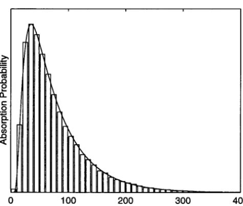
A closely related distribution is that of the absorption tions. As an additional test, the mean of these absorption times can be compared to that predicted by the diffusion time, the time until fixation or extinction of an allele.
Figure 4 compares the distribution predicted on the approximation. Diffusion theory gives the mean absorp-basis ofNeandseto simulation results forD⫽100,N⫽ tion time in a Wright-Fisher population as a certain 100, m ⫽ 0.001, s ⫽ 0.0001, and an initial allele fre- integral (Ewens1979, Equations 4.22 and 5.47). Numer-quency of 1⁄2. Again there is excellent agreement be- ical evaluation of this integral, withN and s replaced tween the prediction and the outcome of the simula- byNeandse, yields the desired prediction. For the pa-rameters used in the simulations presented in Figure 4, the predicted mean absorption time is 7.76 ⫻ 104 generations. The actual mean in the simulations, 7.62⫻ 104 generations, is close to this. For comparison, the mean predicted in the absence of subdivision is 1.29⫻ 104generations, and without selection the prediction is 8.32⫻104 generations.
Table 1 compares the observed and predicted mean absorption times for a variety of parameter values with an initial allele frequency of1⁄
2. For D⫽100 and N⫽ 100, the simulation results are in excellent agreement with the predictions. All of the observed values are slightly smaller than the predictions, but only by at most a few percent. WithD⫽1000 and a mere 10 individuals per deme, the simulation results are again close to the theoretical predictions, even with strong selection and weak migration. For smaller numbers of demes this agreement deteriorates somewhat as migration becomes weak, as expected because the predictions involve the assumption thatD is large. However, even with as few
Figure4.—The distribution of time until absorption
(fixa-tion or extinc(fixa-tion) in 50,000 simula(fixa-tions (bars), compared to as 10 demes, the observed means differ from the predic-a theoreticpredic-al prediction (curve). The simulpredic-ation ppredic-arpredic-ameters tions by⬍20%.
were as follows:D⫽100, N⫽ 100,m⫽ 0.001,s⫽ 0.0001.
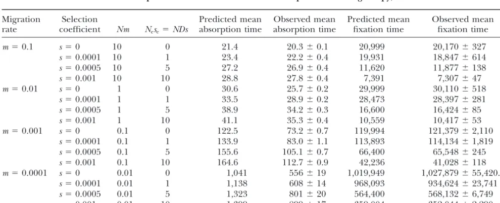
Table 2 shows results for alleles starting out at a single The initial allele frequency was1⁄
2. The predicted distribution
copy. For the higher migration rates the mean absorp-is based on iteration of the transition matrix for a
TABLE 1
Predicted and observed mean absorption times for an initial allele frequency of1⁄ 2
No. of Deme Migration Selection Predicted mean Observed mean
demes size rate coefficient Nm Nese⫽NDs absorption time absorption time
D⫽100 N⫽100 m⫽0.1 s⫽0.0001 10 1 13,579 13,497⫾69
s⫽0.0005 10 5 6,656 6,615⫾24
s⫽0.001 10 10 3,911 3,879⫾11
m⫽0.01 s⫽0.0001 1 1 19,399 19,246⫾98
s⫽0.0005 1 5 9,508 9,362⫾35
s⫽0.001 1 10 5,587 5,442⫾16
m⫽0.001 s⫽0.0001 0.1 1 77,594 76,195⫾248
s⫽0.0005 0.1 5 38,033 37,013⫾140
s⫽0.001 0.1 10 22,347 21,168⫾62
m⫽0.0001 s⫽0.0001 0.01 1 659,553 645,863⫾6,572
s⫽0.0005 0.01 5 323,283 314,510⫾2,432
s⫽0.001 0.01 10 189,951 181,408⫾773
D⫽1000 N⫽10 m⫽0.01 s⫽0.001 0.1 10 22,347 21,957⫾89
m⫽0.001 s⫽0.001 0.01 10 189,951 190,847⫾1,700
D⫽30 N⫽100 m⫽0.001 s⫽0.001 0.1 3 16,146 15,064⫾71
m⫽0.0001 s⫽0.001 0.01 3 137,241 126,867⫾587
D⫽10 N⫽100 m⫽0.1 s⫽0.001 10 1 1,358 1,345⫾7
m⫽0.01 s⫽0.001 1 1 1,940 1,837⫾10
m⫽0.001 s⫽0.001 0.1 1 7,759 6,728⫾39
m⫽0.0001 s⫽0.001 0.01 1 65,955 55,399⫾329
m⫽0.00001 s⫽0.001 0.001 1 647,913 571,948⫾15,587
the lower migration rates the observed means are spread to other demes, and the time to loss is similar to that in a population of sizeN. A number more infor-smaller than the predictions. This phenomenon has
nothing to do with selection; it occurs even in its ab- mative than the mean absorption time is the mean time until fixation (conditional on eventual fixation rather sence. It reflects the fact that extinction, the usual fate
of an allele present in a single copy, occurs very quickly. than on loss). Observed values of this quantity are com-pared to predictions in Table 2 [predicted values were When migration is weak, quasi-equilibrium cannot be
achieved this rapidly. In the limit of very low migration, calculated according toKimuraandOhta(1969, Equa-tion 17), withsesubstituted forsand adjustments made extinction almost always occurs before the allele can
TABLE 2
Predicted and observed mean absorption and fixation times for an allele present in a single copy, withD⫽100 andN⫽100
Migration Selection Predicted mean Observed mean Predicted mean Observed mean
rate coefficient Nm Nese⫽NDs absorption time absorption time fixation time fixation time
m⫽0.1 s⫽0 10 0 21.4 20.3⫾0.1 20,999 20,170⫾327
s⫽0.0001 10 1 23.4 22.2⫾0.4 19,931 18,847⫾614
s⫽0.0005 10 5 27.2 26.9⫾0.4 11,620 11,877⫾138
s⫽0.001 10 10 28.8 27.8⫾0.4 7,391 7,307⫾47
m⫽0.01 s⫽0 1 0 30.6 25.7⫾0.2 29,999 30,110⫾518
s⫽0.0001 1 1 33.5 28.9⫾0.2 28,473 28,397⫾281
s⫽0.0005 1 5 38.9 34.2⫾0.3 16,600 16,424⫾85
s⫽0.001 1 10 41.1 35.3⫾0.4 10,559 10,417⫾53
m⫽0.001 s⫽0 0.1 0 122.5 73.2⫾0.7 119,994 121,379⫾2,110
s⫽0.0001 0.1 1 133.9 83.0⫾1.1 113,893 114,134⫾1,819
s⫽0.0005 0.1 5 155.6 105.1⫾0.7 66,400 65,548⫾245
s⫽0.001 0.1 10 164.6 112.7⫾0.9 42,236 41,028⫾118
m⫽0.0001 s⫽0 0.01 0 1,041 556⫾19 1,019,949 1,027,879⫾55,420.2
s⫽0.0001 0.01 1 1,138 608⫾14 968,093 934,624⫾23,741
s⫽0.0005 0.01 5 1,323 801⫾20 564,400 568,132⫾6,749
for haploidy]. The mean fixation times in the simula- panmictic. Both the mean and the variance of the change in allele frequency are approximately propor-tions are in excellent agreement with these predicpropor-tions:
the observed means are all within a few percent of the tional to the mean of xi(1⫺ xi). Subdivision therefore
slows down drift and selection by the same factor. While predicted values, even when migration rates are small.
In all of the simulations presented above, except seis directly proportional to the mean change in allele frequency,Neis inversely proportional to the variance, where s ⫽ 0, |NDs| ⱖ 1 (NDs ranges from 1 to 100).
so it changes by the same factor but in the opposite Therefore selection has a significant effect on the fate
direction. The quantityNese, which is the ratio of the of the allele in the population as a whole. Thus the
mean to the variance of the change in allele frequency, simulations test the ability of the theory to account for
is unaffected by subdivision. Therefore, as expected selection; had |NDs| been small, the deviation of the
from the results ofMaruyama(1970b, 1974), fixation results from the strictly neutral case would be
insignifi-probabilities are also unaffected by subdivision. How-cant, and the simulations would test only whether the
ever, the rate at which allele frequencies change is de-theory worked well under neutrality. The results
demon-creased. Because the two components of this change, strate that the theoretical approximations work well in
selection and drift, are slowed by the same factor, the the presence of significant selection, so long as |Ns| is
effect of subdivision on the trajectory of allele frequency small compared to one (Nsranges from 0.01 to 0.1 in
is simply a dilation in time. the simulations).
We thank Jon Wilkins for helpful discussions. This work was sup-ported by National Science Foundation grant DEB-9815367 to J.W.
DISCUSSION
Despite the fact that the state of a subdivided
popula-LITERATURE CITED tion cannot be described by a single allele frequency,
Caballero, A., 1994 Developments in the prediction of effective
the trajectory of the overall allele frequency x in an
population size. Heredity73:657–679.
island model (Wright1931) can be described well by
Chesser, R. K., O. E. Rhodes, Jr., D. W. SuggandA. Schnabel,
a one-dimensional diffusion approximation. This is the 1993 Effective sizes for subdivided populations. Genetics135: 1221–1232.
case even in the presence of selection that is strong
Dobzhansky, T., andS. Wright, 1941 Genetics of natural populations.
enough to have a large influence on the probability of
V. Relations between mutation rate and accumulation of lethals in
an allele’s fixation. Furthermore, this diffusion approxi- populations ofDrosophila pseudoobscura.Genetics26:23–51. Ewens, W. J., 1979 Mathematical Population Genetics.Springer-Verlag,
mation is equivalent to that for some idealized panmictic
Berlin.
population. Thus, classical diffusion results for
non-Gillespie, J. H., 1998 Population Genetics: A Concise Guide.The Johns
structured populations may be applied to a structured Hopkins University Press, Baltimore.
Gregorius, H. R., 1991 On the concept of effective number. Theor.
population that conforms to the island model.
Simula-Popul. Biol.40:269–283.
tion results confirm the validity of these approximations.
Kimura, M., 1955a Solution of a process of random genetic drift
The equivalent panmictic population has parameter with a continuous model. Proc. Natl. Acad. Sci. USA41:144–150. Kimura, M., 1955b Stochastic processes and the distribution of gene
values that are different from their counterparts in the
frequencies under natural selection. Cold Spring Harbor Symp.
island model. As is the case for many population-genetic
Quant. Biol.20:33–53.
models, the size of the hypothetical equivalent Wright- Kimura, M., andT. Ohta, 1969 The average number of generations
until fixation of a mutant gene in a finite population. Genetics
Fisher population, Ne, is different from (in this case
61:763–771.
greater than) the size of the actual population. This
Maruyama, T., 1970a Effective number of alleles in a subdivided
state of affairs is familiar in population genetics and is population. Theor. Popul. Biol.1:273–306.
Maruyama, T., 1970b On the fixation probability of mutant genes
the reason for defining effective population size in the
in a subdivided population. Genet. Res.15:221–225.
first place. A less familiar aspect of the present result is
Maruyama, T., 1972a Distribution of gene frequencies in a
geo-that the selection coefficient in the hypothetical equiva- graphically structured finite population. I. Distribution of neutral
genes and of genes with small effect. Ann. Hum. Genet. 35:
lent population is different from that in the actual
popu-411–423.
lation. This motivates the definition, by analogy to
effec-Maruyama, T., 1972b Distribution of gene frequencies in a
geo-tive population size, of the effecgeo-tive selection coefficient graphically structured population. 3. Distribution of deleterious
genes and genetic correlation between different localities. Ann.
se. In the present case, se ⬍ s. Specifically, subdivision
Hum. Genet.36:99–108.
lowers the effective selection coefficient by the same
Maruyama, T., 1972c Distribution of gene frequencies in a
geo-factor by which it raises effective population size. This graphically structured population. II. Distribution of deleterious
genes and of lethal genes. Ann. Hum. Genet.35:425–432.
factor depends on the product of deme size and
migra-Maruyama, T., 1974 A simple proof that certain quantities are
inde-tion rate (Nm), which determines the extent of
differen-pendent of the geographical structure of population. Theor.
tiation among the demes. Popul. Biol.5:148–154.
Maruyama, T., andM. Kimura, 1980 Genetic variability and
effec-The effects of subdivision on Ne and se both result
tive population size when local extinction and recolonization
from the fact that the expected value of the within-deme
of subpopulations are frequent. Proc. Natl. Acad. Sci. USA77:
quantity xi(1 ⫺ xi) is smaller than the quantity x(1⫺ 6710–6714.
Nei, M., andN. Takahata, 1993 Effective population size, genetic
diversity, and coalescence time in subdivided populations. J. Mol. Takahata, N., 1991 Genealogy of neutral genes and spreading of selected mutations in a geographically structured population. Evol.37:240–244.
Nordborg, M., 1997 Structured coalescent processes on different Genetics129:585–595.
Wang, J., andA. Caballero, 1999 Developments in predicting the time scales. Genetics146:1501–1514.
Rannala, B., 1996 The sampling theory of neutral alleles in an island effective size of subdivided populations. Heredity82:212–226. Whitlock, M. C., andN. H. Barton, 1997 The effective size of a population of fluctuating size. Theor. Popul. Biol.50:91–104.
Rousset, F., 2001 Inferences from spatial population genetics, pp. subdivided population. Genetics146:427–441.
239–269 inHandbook of Statistical Genetics,edited by D. J.Balding, Wright, S., 1931 Evolution in Mendelian populations. Genetics16: M. J.Bishopand C.Cannings. John Wiley & Sons, Chichester, 97–159.
England. Wright, S., 1939 Statistical Genetics in Relation to Evolution(Actualites
Santiago, E., andA. Caballero, 1995 Effective size of populations Scientifiques et Industrielles, 802: Exposes de Biometrie et de la
under selection. Genetics139:1013–1030. Statistique Biologique XIII). Hermann et Cie, Paris.
Slatkin, M., 1977 Gene flow and genetic drift in a species subject Wright, S., 1940 Breeding structure of populations in relation to to frequent local extinctions. Theor. Popul. Biol.12:253–262. speciation. Am. Nat.74:232–248.
Slatkin, M., 1981 Fixation probabilities and fixation times in a Wright, S., 1969 Evolution and the Genetics of Populations, Vol. 2: The
subdivided population. Evolution35:477–488. Theory of Gene Frequencies.University of Chicago Press, Chicago.
Slatkin, M., 1991 Inbreeding coefficients and coalescence times.