DOI: 10.1534/genetics.106.061960
On the Generalized Poisson Regression Mixture Model for Mapping
Quantitative Trait Loci With Count Data
Yuehua Cui,*
,1Dong-Yun Kim* and Jun Zhu
†*Department of Statistics and Probability, Michigan State University, East Lansing, Michigan 48824 and†College of Agricultural and Biotechnology, Zhejiang University, Hangzhou, Zhejiang 310029, People’s Republic of China
Manuscript received June 13, 2006 Accepted for publication September 24, 2006
ABSTRACT
Statistical methods for mapping quantitative trait loci (QTL) have been extensively studied. While most existing methods assume normal distribution of the phenotype, the normality assumption could be easily violated when phenotypes are measured in counts. One natural choice to deal with count traits is to apply the classical Poisson regression model. However, conditional on covariates, the Poisson assumption of mean– variance equality may not be valid when data are potentially under- or overdispersed. In this article, we propose an interval-mapping approach for phenotypes measured in counts. We model the effects of QTL through a generalized Poisson regression model and develop efficient likelihood-based inference pro-cedures. This approach, implemented with the EM algorithm, allows for a genomewide scan for the ex-istence of QTL throughout the entire genome. The performance of the proposed method is evaluated through extensive simulation studies along with comparisons with existing approaches such as the Poisson regression and the generalized estimating equation approach. An application to a rice tiller number data set is given. Our approach provides a standard procedure for mapping QTL involved in the genetic control of complex traits measured in counts.
M
ODERN biological techniques make it possible to detect the abundant variation of molecular poly-morphisms that segregate in most species in nature. Consequently, it is possible to detect quantitative trait loci (QTL) underlying quantitative variation of certain traits and to map their chromosomal locations through-out the entire genome using statistical methods (Mackay 2001). Given the recent intriguing result of gene cloning from rice on the basis of QTL mapping results (Liet al.2006), QTL mapping is still proven to be an important tool for gene discovery in the postgenomic era. Therefore, there is a great demand to develop ef-ficient statistical methods to improve the precision and power of QTL mapping, not only for continuous traits, but also for discrete traits such as those measured in counts.Most current statistical methods for QTL mapping in experimental crosses date back to the seminal mapping article of Landerand Botstein(1989). Since then, this work has been extended and improved by a number of statistical methods, for example, composite interval map-ping (Zeng1994) and multiple-interval mapping (Kao
et al. 1999). However, most of the existing methods developed so far assume that the phenotypic trait be normally distributed. This assumption is easily violated when the phenotype of interest shows nonnormal
char-acteristics, for instance, pertaining to survival time (Diao
et al.2004) or displaying a binary characteristic (Xuand Atchley1996).
Another type of data often observed in real experi-ments is count data where the phenotype of interest is measured in counts. For example, the number of roots generated in a plant (Lallet al.2004), CD4 T cell counts in a human study (Hallet al.2002), and the number of cholesterol gallstones formed in mice (Wittenburg
et al. 2003) are all examples of phenotypes measured in counts. The distribution of these types of data is generally skewed, especially when the mean is compar-atively small. Tilquinet al.(2001) proposed to perform a mathematical transformation of count data and then apply a standard QTL mapping approach such as least squares (Haley and Knott 1992), maximum likeli-hood (Landerand Botstein1989), or a nonparamet-ric approach (Kruglyakand Lander1995). However, the nature of the data distribution is still not incorpo-rated and consequently the mapping power might be affected. Due to the lack of an efficient statistical method, the standard QTL mapping approach assum-ing normally distributed phenotypes is still beassum-ing ap-plied (Lallet al.2004).
When the sampling variance of a count variableYis significantly greater or less than that predicted by an expected probability distribution,Yis said to be over- or underdispersed, respectively. A natural way to analyze regular count data is to use a Poisson regression model where the Poisson mean can be modeled as a function 1Corresponding author: Department of Statistics and Probability,
Michigan State University, A-411 Wells Hall, East Lansing, MI 48824. E-mail: [email protected]
of linear predictors through the log link function in a generalized linear model (GLM) setting (McCullagh and Nelder 1989). Using parametric approaches by applying Poisson distribution in QTL mapping has been previously proposed (Rebaı¨ 1997; Shepel et al. 1998; Sen and Churchill 2001). These approaches were built on the maximum-likelihood framework (Shepel
et al. 1998), least-squares-based regression framework (Rebaı¨ 1997), and Bayesian framework (Sen and Churchill2001), and each one displays its own merits in handling count data in QTL mapping. However, if dispersion occurs, ignoring it will result in biased pa-rameter estimates, which may lead to incorrect conclu-sions and inferences (Wang 1994). Therefore, these approaches are greatly limited when the underlying data are potentially dispersed.
When count data are dispersed, one can apply a non-parametric approach (Kruglyak and Lander 1995) using its nice distribution-free property. However, one of its major disadvantages is that it does not provide QTL-effect estimation and hence greatly restricts its util-ity for inference. Moreover, it is based on the Wilcoxon rank-sum test and chooses to rank tied individuals at random. This also greatly restricts its application when the number of ties is high, especially for count data (Rebaı¨1997). McCullaghand Nelder(1989) suggest modeling mean and dispersion jointly as a way to take possible dispersion into account. The GLM was later applied to a QTL mapping study using a generalized estimating equation (GEE) approach (Lange and Whittaker2001; Thomson2003). The GEE approach shows its merits in handling dispersion. However, since the GEE approach does not assume a full probabil-ity model, a misspecified variance may have an influ-ence on the efficiency of the parameter estimates and a likelihood-based inference procedure cannot be ap-plied directly. Wanget al.(1996) suggest modeling data with a mixed Poisson regression model to take data dispersion into account. Famoye (1993) proposed a generalized Poisson regression model in which the dis-persion parameter can be directly estimated and tested. Neither of these two approaches has been applied in QTL mapping studies.
In this article, we propose a rigorous extension of the interval-mapping approach to count traits. We model the QTL effects through a generalized Poisson regression model (Famoye1993) and develop efficient likelihood-based inference procedures. Residual analysis and good-ness-of-fit tests are proposed to check the model fitting. This approach, implemented with the EM algorithm, allows for a genomewide scan for the existence of QTL throughout the entire genome. Extensive simulation studies are performed to evaluate the statistical behavior of the approach. Comparisons with the GEE approach and the Poisson regression are also given on the basis of simulations. An application to a rice tiller number data set is provided in which several QTL are detected to
affect tiller growth. Our approach provides a standard procedure for mapping QTL involved in the genetic control of complex traits measured in counts.
MODELS
Generalized Poisson regression model:Suppose that
Yiis a count response variable that follows a generalized
Poisson distribution (Famoye 1993). The probability function ofYiis given by
pðYi¼yijli;fÞ
¼ li 11fli
yið11fy
iÞyi1
yi!
exp lið11fyiÞ 11fli
; yi¼0;1;. . .;
ð1Þ
where li is the mean of the function and can be
ex-pressed as a function of genetic and nongenetic factors;
i.e.,li ¼liðxiÞ ¼expðx9ibÞ, wherexiis ap-dimensional
vector of covariates including genetic and nongenetic factors,bis ap-dimensional vector of regression param-eters, andfis a dispersion parameter.
The generalized Poisson regression (GPR) model (1) is a generalization of the standard Poisson regression (PR) model. When the dispersion parameterf¼0, the probability function in (1) reduces to the PR model. Whenf.0, the GPR model represents count data with overdispersion and when f, 0, the GPR model rep-resents count data with underdispersion. Therefore, the GPR model shows more flexibility in modeling count data when the underlying data show varying degrees of dispersion. Since the parameterfis restricted to 11 fli.0 and 11fyi.0, the model is also called the
re-stricted generalized Poisson regression model (Famoye 1993).
The mean of the response in the GPR model is given byE(Yijli,f)¼liand the variance is given byV(Yijli,
f)¼li(11fli)2. Clearly, whenf.0, the variance is
overdispersed and when2/li,f,0, the variance is
underdispersed. The GPR model is very useful for mod-eling count data, especially when mean and variance differ.
Interval-mapping approach: In this section, we de-velop an interval-mapping method for potentially dis-persed count traits in a backcross population. Expanding the results to other crosses such as an F2or a recombinant
inbred line (RIL) is straightforward. Suppose that there is a putative QTL that is segregating with two allelesQand
qin a backcross population of sizen, initiated with two contrasting inbred lines. The QTL is assumed to be responsible for the quantitative variation of the pheno-type measured in counts. Data are randomly collected, which include a set of genetic markers with a known genetic linkage map and set of phenotype data.
For simplicity, we ignore nongenetic covariates and consider only the genetic covariates. Letxi¼1 or 0
effects of the QTL genotype on the count trait such that, conditional on the QTL genotypeGi, the mean of the
GPR model can be expressed as
lijGi ¼expðx9ibÞ ¼
expðm1aÞ forQQ
expðmÞ forQq; ð2Þ
whereb¼(m,a) in whichmis the overall genetic effect, andais the additive genetic effect.
Statistical methods for mapping QTL on the basis of a mixture model have been previously developed (Landerand Botstein1989). In the mixture model, each observationyis assumed to have arisen from one of
jcomponents (QTL genotypes), with each component being modeled by a probability distribution function, for example, a generalized Poisson regression function in the current setting. At each locus, the conditional probability of QTL genotype j given on the flanking markersMifor individual ican be calculated, which is
expressed aspijj¼Pr(xi¼jjMi) (i¼1, . . . ,n), wherenis
the total sample size andjtakes value 1 or 0 depending on whether the QTL genotype isQQorQq(Lynchand Walsh1998). The conditional probability is considered as the mixture proportion in the mixture model. For the backcross family, the mixture model has the form
fðyijli;fÞ ¼pij1p1ðyijlij1;fÞ1pij0p0ðyijlij0;fÞ: ð3Þ
From the mixture distribution, we can easily compute the unconditional mean and variance ofYi, which are
expressed as
mi ¼EðYiÞ ¼EðEðYijliÞÞ ¼
X1
j¼0
pijjlijj ð4Þ
and
VðYiÞ ¼EðVðYijliÞÞ1VðEðYijliÞÞ
¼X 1 j¼0
fl2ijj1lijjð11flijjÞ2g ½EðYiÞ2: ð5Þ
Assuming independent observations, the log-likeli-hood function given the phenotypeyand marker data
Mcan be expressed as
‘nðb;fjy;MÞ
¼X n
i¼1
logfpij1p1ðyijlij1;fÞ1pij0p0ðyijlij0;fÞg: ð6Þ
The parameters specifying functionp1are (m,a,f)
with lij1 ¼ exp(m1a) and the parameters specifying
functionp0are (m,f) withlij0¼exp(m).
Parameter estimation:DefineV¼ ðb;fÞ ¼ ðm;a;fÞ, which contains the genetic parameters and dispersion parameter. The maximum-likelihood estimate (MLE) ˆV
forVis such that it solves the partial-derivative equation with respect to the rth parameter contained in V:
@‘n(V)/@Vr¼0. In practice, we treat the positions of
QTL, t, as known parameters rather than unknown, although their MLEs can also be obtained through iterative steps. We can then use a grid search approach to estimate the QTL positions. By hypothesizing a QTL every 1 or 2 cM at marker intervals, the landscape of log-likelihood test statistics throughout the entire genome can be obtained. The positions corresponding to the peak of the landscape across a linkage group are the MLEs of the QTL positions. Therefore, a computational algorithm can be formulated as follows. For any fixed QTL position, t, the EM algorithm (Dempster et al. 1977) is used to find the restricted MLE ˆVðtÞ, with the Newton–Raphson algorithm employed in the M-step (detailed instructions are given in theappendix). Then obtain ˆt by varyingt over an interval with a small in-crement of 1 or 2 cM at a time.
With a backcross design, we have two mixture com-ponents. For a fixed number of mixtures, asymptotic normality ofpffiffiffinððmˆ;aˆ;fˆÞ ðm;a;fÞÞcan be proved un-der standard regularity conditions (Lehmann 1983). However, as restricted by the condition 11fyi.0, the
parameterfis bounded below by the observed data set. Iffreaches the lower bound, the asymptotic normality for fmay not be satisfied. The approximate standard errors of the estimates can be obtained from the by-product of the Newton–Raphson algorithm. Applying Wald’s (1949) consistency argument and using the techniques developed in Chen and Chen (2005), we can prove the consistency of the MLEs ofVunder the GPR mixture model. If a QTL exists in an interval,i.e.,
a6¼0, the MLE of QTL positiontis also consistent.
Hypothesis test:The presence of QTL responsible for the variation of the count phenotype can be tested by using the following hypotheses:
H0:a¼0
H1:a6¼0: ð7Þ
The test statistic for testing the above hypotheses is calculated as the log-likelihood-ratio test statistic (LR) of the full model (H1) over the reduced model (H0),
LR¼ 2 log½LðV~Þ LðVˆÞ; ð8Þ
where V~ and ˆV denote the MLEs of the unknown parameters under H0and H1, respectively. Because of
the mixture model, the regularity conditions for asymp-toticx2-distribution of the LR do not hold. To find the threshold value, we use the permutation test proposed by Churchilland Doerge(1994).
MODEL IMPLEMENTATION
Poisson regression models may be applied to a given data set. A natural question arises: Which model should one adopt to fit the data for QTL analysis? This is es-sentially a model selection problem. Two widely used model selection criteria are Akaike’s Information Cri-terion (AIC) (Akaike1974) and the Bayesian Informa-tion Criterion (BIC) (Schwarz 1978). Quantitatively, the BIC puts more penalty on the log-likelihood func-tion and the model selected by the BIC is more parsi-monious. Here we define the AIC and the BIC criteria for the mixture model as
AIC¼ 2 lnLðVˆ jyÞ12p ð9Þ
and
BIC¼ 2 lnLðVˆ jyÞ1plogðnÞ; ð10Þ
wherepis the number of free parameters in the defined model. The model with the smallest AIC or BIC value is selected as the best.
Dispersion test: The GPR model reduces to the Poisson regression model when the dispersion parame-terfvanishes. To assess the adequacy of the GPR model over the Poisson regression model, and to determine whether the data are over- or underdispersed with re-spect to the generalized Poisson regression model, a test for the dispersion parameter can be formulated as follows:
H0:f¼0
H1:f6¼0: ð11Þ
When the lower bound for ˆfis not reached, a Wald-type test can be conducted in which ˆf=OsˆðfÞ may asymptotically follow a standard normal distribution. Further theoretical investigation is needed to demon-strate the validity of the Wald test forfunder the mix-ture distribution framework. Alternatively we can apply the likelihood-ratio test in which the threshold is deter-mined using permutation tests. The sign of significant test statistics suggests over- or underdispersion, where negative estimates indicate underdispersion and posi-tive estimates indicate overdispersion. Meanwhile, sig-nificance of the test provides evidence of a better fit for the GPR model over the PR model.
Residual analysis and goodness-of-fit: After model selection and a GPR model is fitted, it is essential to check the quality of the fit. One way to check the quality of fits is to perform a residual analysis. For this purpose, we consider a Pearson or a deviance residual to check the model fit. The Pearson residual for theith observa-tion is defined as
rpi ¼
yimˆi
OVˆðyiÞ
; ð12Þ
where ˆmi andVˆðyiÞcan be obtained from (4) and (5)
by replacing the parameters by the MLEs. The sum
of squared Pearson residuals, X2, gives the Pearson goodness-of-fit statistic for the GPR mixture model.
The deviance residual is defined as
rdi ¼signðyimˆiÞ ffiffiffiffi di p
; ð13Þ
where di¼2ð‘ðyi;fˆ;yiÞ ‘ðmˆi;fˆ;yiÞÞ, and ‘ðyi;fˆ;yiÞ ¼
fðyijyi;fˆÞ, and ‘ðmˆi;fˆ;yiÞ is the log likelihood of the
generalized Poisson regression mixture model for yi.
The goodness-of-fit of the generalized Poisson regres-sion mixture model can be measured by the deviance
D¼Pni¼1di.
The above two residuals asymptotically follow the stan-dard normal distribution asn/‘. Therefore, large re-siduals may indicate poorly fitting observations (Pierce and Schafer 1986). An index plot of these residuals may be used for detection of potential outliers.
After calculating the residuals, we can also use these residuals to test the goodness-of-fit for the GPR mixture model. The Pearson’s statisticX2and the deviance sta-tistic D are asymptotically distributed as x2
nm under
the null hypothesis, wheremis the number of free pa-rameters under the alternative (Wang et al. 1996). A large value ofX2orDindicates poor fit.
We can also apply the techniques developed by Wang
et al.(1996) to evaluate how theith observation affects a set of parameter estimates. We define the following quantity as the influential estimate (IE) for individuali, which has the form
wi¼ 1
m
Xm
k¼1
jVˆkVˆ ðiÞ k j
seðVˆkÞ ; ð14Þ
where ˆVk and ˆV
ðiÞ
k are the MLEs of the GPR mixture
model based on the complete data set ofnindividuals and on the dataset ofn1 individuals excluding theith individual, respectively; and mis the total number of parameters in the model. The IE calculated for in-dividualican be interpreted as the average relative co-efficient changes for a set of estimates and is useful for assessing the effect of parameter estimates by exclusion of theith observation (Wanget al.1996). Therefore, a relatively large value ofwiindicates a potential
influen-tial observation that might cause instability in model fitting. An index plot ofwmay be used for detection of the influential point.
SIMULATION
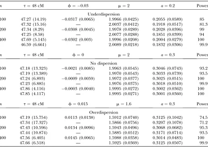
a backcross population with which a 100-cM-long link-age group composed of six equidistant markers is con-structed. A putative QTL that affects the phenotype of interest is located at 48 cM from the first marker on the linkage group. The Haldane map function is used to convert the map distance into the recombination fraction. To test the model performance, we simulate data with different specifications, namely different sam-ple sizes (n ¼ 100, 200, and 400), and different pat-terns of dispersion using the proposed GPR mixture model.
In each simulation scenario, 1000 Monte Carlo repeti-tions are performed. For each Monte Carlo sample, the EM algorithm is used to obtain the MLEs of parameters. Table 1 tabulates the MLEs of all parameter estimates. The square root of the mean square error (SMSE) is given in parentheses, which provides a measure of pre-cision for each parameter estimate. The result listed in the first row for each given sample size is obtained using the GPR model, and the one in the second row is obtained using the regular PR model. In general, the GPR model can provide reasonable estimates of the QTL positions (t) and effects of various kinds, with es-timation precision depending on sample size and
dis-persion pattern. As expected, the precision of QTL parameters increases with increased sample size. For example, the SMSE of the mean parameteradecreases by more than twofold under different dispersion pat-terns when the sample size increases from 100 to 400. Meanwhile, as the sample size increases, the mapping power also increases (Table 1).
Under different dispersion patterns, all the parame-ters can be reasonably estimated with high precision with the GPR model, which suggests the robustness of the model and good convergence rate of parameters. A minor difference is observed for the QTL location estimates in which slightly higher precision is observed when data show no dispersion. When the sample size is small (i.e.,n¼100), high mapping power is observed when data show no dispersion compared to dispersed data (Table 1). For example, the power is 93.2% for no dispersion data compared to 74.5% for overdispersed data and 85% for underdispersed data with the sample size 100. The reduction of mapping power is possibly due to extra data variation caused by under- or over-dispersion. The difference is not so notable when sample size increases to 200, which suggests that a rea-sonable sample size of 200 is needed in practice. TABLE 1
The mean MLEs with their square-root mean square errors (SMSEs) (in parentheses) of the parameters estimated from 1000 simulation replicates with different dispersion patterns
n t¼48 cM f¼ 0.03 m¼2 a¼0.2 Power
Underdispersion
100 47.27 (14.19) 0.0317 (0.0065) 1.9966 (0.0425) 0.2055 (0.0589) 85 47.32 (15.16) — 2.0037 (0.0412) 0.1918 (0.0517) 81.3 200 47.34 (8.29) 0.0308 (0.0045) 1.9978 (0.0289) 0.2028 (0.0396) 99
47.25 (8.58) — 2.0077 (0.0288) 0.1851 (0.0399) 94 400 47.69 (5.145) 0.0302 (0.003) 1.9996 (0.0208) 0.2004 (0.0279) 100 46.59 (6.661) — 2.0089 (0.0218) 0.1832 (0.0306) 99.9
n t¼48 cM f¼0 m¼2 a¼0.3 Power
No dispersion
100 47.18 (13.323) 0.0021 (0.0085) 1.9963 (0.0545) 0.3046 (0.0743) 93.2 47.19 (13.389) — 1.9970 (0.0543) 0.3033 (0.0739) 93.5 200 47.24 (6.893) 0.0009 (0.0059) 1.9972 (0.0377) 0.3025 (0.0515) 100
47.23 (6.885) — 1.9976 (0.0375) 0.3018 (0.0510) 99.9 400 47.86 (4.116) 0.0003 (0.0040) 1.9995 (0.0272) 0.3002 (0.0362) 100
47.85 (4.117) — 1.9995 (0.0271) 0.3001 (0.0360) 100
n t¼48 cM f¼0.015 m¼1.6 a¼0.3 Power
Overdispersion
100 47.19 (15.754) 0.0113 (0.0138) 1.5912 (0.0740) 0.3125 (0.1042) 74.5 47.34 (17.327) — 1.5866 (0.0756) 0.3207 (0.1078) 71.2 200 47.43 (10.596) 0.0134 (0.0096) 1.5943 (0.0496) 0.3068 (0.0682) 95.3 47.44 (10.874) — 1.5885 (0.0512) 0.3171 (0.0714) 93.5 400 47.56 (6.405) 0.0145 (0.0065) 1.5988 (0.0358) 0.3014 (0.0483) 100
Comparisons between the GPR and PR model are summarized in Table 1, where the underlying data are simulated using the GPR model. When data are poten-tially dispersed, the GPR model outperforms the PR model with increased precision for QTL location and other genetic parameter estimation as well as increased testing power. The differences are more notable when sample size is small. For example, the power is 85% using the GPR model compared to 81.3% using the PR model with a sample size of 100 from underdispersed data. We also observe a larger bias for the additive effect
a using the PR model compared to the GPR model, which could lead to biased inference. When data are not dispersed, both models perform similarly.
Comparisons of the current approach with the GEE-type approach (Langeand Whittaker2001) are summarized in Figures 1 and 2. Figure 1 shows the com-parisons based on the power and type I error rate. Data are simulated using the GPR model and are then ana-lyzed using both approaches. The power and type I error are calculated on the basis of the 5% nominal level from the permutation test (Churchilland Doerge1994). When data are dispersed and sample size is small (100 say), the GPR approach has higher power than the GEE approach. As sample size increases to$200, these two approaches are comparable. Both approaches underes-timate the type I error rate when sample size is small and data are dispersed. When sample size increases to 400, the GEE approach overestimates the type I error and performs poorly compared to the GPR approach. When data are not dispersed, the difference in power is not significant, but it is not so for the type I error.
A boxplot of the QTL position estimates is given in Figure 2, which displays the interquantile and the range
of the estimated position. Outliers are indicated by asterisks. The notch indicates a robust estimate of the uncertainty about the median. The dotted vertical line represents the true QTL location. In all simulation studies, the GPR approach gives more efficient esti-mates of the QTL position than the GEE approach.
APPLICATION
The proposed model is employed to reanalyze a real data set of rice tiller number (Yan et al. 1998). Two inbred lines, semidwarf IR64 and tall Azucena, were crossed to generate an F1progeny population. By
dou-bling haploid chromosomes of the gametes derived from the heterozygous F1, a doubled-haploid (DH)
pop-ulation of 123 lines was founded (Huanget al.1997), which is genetically equivalent to a backcross popula-tion. A genetic linkage map was constructed using 175 genetic markers, with a total length of 2005 cM, rep-resenting a good coverage of 12 rice chromosomes.
The 123 DH lines were planted in a completely randomized design with two replications. Each replicate was divided into different plots, each containing eight plants per line. Starting from 10 days after transplant-ing, tiller numbers were measured every 10 days for five central plants in each plot until all lines had headed. The tiller numbers were averaged from the two repli-cates. Given that tiller number can be only an integer, the averaged tiller number was rounded to the nearest integer for QTL analysis. Since the majority of individ-uals have only one tiller and the rest have two tillers at day 10 after rounding, the data do not provide enough variability to fit the GPR model. Only data beginning at day 20 were subject to QTL mapping study.
Three types of statistical model are applied, namely a model with regular Poisson regression, a model with the newly proposed generalized Poisson regression, and the GEE approach (Langeand Whittaker2001). The PR and GPR approaches lead to a significantly different LR profile throughout the genome and consequently a larger number of QTL are identified by the GPR than by the PR model. There is only one genomewide signifi-cant QTL identified by the GEE approach, located on chromosome 5 before day 50. After day 50, no genome-wide significant QTL are identified. Also, the location of the identified QTL by the GEE approach is completely different from the ones detected using the GPR model. Both the dispersion test and the goodness-of-fit test show that data are underdispersed. Therefore, we focus only on the results obtained by the GPR model in this section.
By genomewide scanning for QTL at every 2 cM within each marker interval across 12 rice chromo-somes, our model has identified six major QTL that trigger effects on tiller growth. As shown by the genome-wide LR profile plot in Figure 3, QTL located on chro-mosomes 2, 5, and 8 are significant only at the 5% chromosomewide level and QTL located on chromo-some 4 (marker interval RZ565–RZ675) show genome-wide significance on the basis of the critical thresholds determined from 1000 permutation tests. Both QTL located on chromosome 3 show genomewide signifi-cance at days 40 and 70 but show chromosomewide
significance at the other periods. One of the possible reasons that these QTL do not show genomewide sig-nificance during the whole study period might be due to small sample size. As revealed by the simulation study, the mapping power is greatly affected by sample size when data are potentially dispersed.
It is noteworthy that different QTL are involved in the control of tiller growth during different stages of rice development (Figure 3). A QTL detected on chromo-some 3 (marker interval CDO337–RZ337A) has triggered continuous effects on tiller growth since activation. A QTL detected on chromosome 8 is obviously an early locus that affects tiller growth only during the first 30 days. As this QTL is switched off, some other QTL are activated to regulate tiller development. For example, a QTL on chromosome 5 becomes operational at day 40 but only functions for a short period of time and is switched off after day 50. Another QTL on chromo-some 2 is then switched on at day 50 and continuously functions. Following the turn-off of the QTL on chro-mosome 5, the QTL located on chrochro-mosome 4 starts to function from day 70.
5% genomewide level are marked by double asterisks. Clearly shown in Table 2, for individuals carrying geno-typeQQ, QTL on chromosomes 2 and 5 trigger a posi-tive effect on tiller growth while the rest of the QTL located on chromosomes 3, 4, and 8 exert a negative effect on tiller growth. Depending on the need in breed-ing, a scientist may pay particular attention to those QTL.
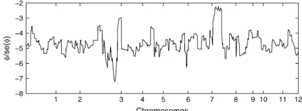
We pick one QTL located at chromosome 3 within marker interval RZ519–Pgi-1 at day 40 to demonstrate the model implementation. The sample mean is 11.07 and the sample variance is 6.33, which indicates po-tential underdispersion with respect to Poisson distri-bution. This conjecture is further confirmed by the dispersion test (11) as shown in Figure 4. As revealed by the real data analysis, the parameterfnever reaches the lower bound across all the linkage locations, hence we can apply Wald’s test. The ratios of dispersion parame-ters with respect to their standard errors are all, 2 across all loci of the entire genome. The differences of the AIC and BIC values when fitting the data with the GPR mixture model and the PR mixture model are also calculated across the entire genome. As clearly shown in Figure 5, the differences are always negative for both criteria, which indicates that the GPR mixture model has better fit than PR mixture model at all loci.
We also calculated the deviance and Pearson residuals as well as the influential estimates for the QTL detected on chromosome 3 at marker interval RZ519–Pgi-1 at day 40. The Pearson and the deviance goodness-of-fit statisticX2andDare 3.45 and 86.48, respectively, with 88 d.f. These values are less than the upper 95% critical point of thex2
88-distribution, suggesting that there is no
evidence of lack of fit. The Pearson and the deviance residuals are displayed in Figure 6. The Pearson
re-siduals appear to be normally distributed. However, the deviance residuals show that some of the data may be potential outliers such as the 47th and 53rd observa-tions. On omitting these observations, the deviance is reduced by 0.2, while theX2is reduced by 0.46. This im-plies that these observations are possible outliers, but they may not have a significant impact on the overall fit of the GPR model.
To check which observations are influential points on parameter estimates, we calculated the influential esti-mates w, which are displayed in Figure 6. As shown, observations 47 and 53 are potentially influential. If we omit these two observations, the overall genetic effect estimatemdoes not change, but the additive and disper-sion parameter estimates change by 11 and 17%, re-spectively. By further omitting three more observations (the 2nd, 71st, and 82nd), we observe a change of 33 and 16%, respectively, for additive and dispersion param-eters. However, omitting these observations does not affect the likelihood-ratio test statistic as much.
EXTENSIONS
model to multiple-QTL analysis on the basis of these two approaches. An extension of the current approach to a random-mean model is also given.
Composite-interval mapping:The basic idea of CIM is to incorporate multiple-regression analysis into interval mapping by conditioning on markers outside an inter-val of interest. By controlling the background markers effect, the precision and power of QTL mapping is
improved. To extend the original CIM model to count traits, we consider the following mean function,
lijGi¼expðxib1 X
l6¼j;j11
xlblÞ; ð15Þ
where jandj11 represent two flanking markers bor-dering the putative QTL, andxlis the indicator variable
for the selected background marker genotype, which
Figure4.—The ratio of the dispersion param-eter ˆfwith its standard error across the entire 12 chromosomes for tillers measured at day 40. TABLE 2
Estimated genetic effects and their asymptotic standard errors (in parentheses) of QTL detected for the tiller number of the DH population at different stages
Chromosome Marker interval Day m a f LR
2 RG654–RG256 50 2.264 (0.038) 0.144 (0.048) 0.027 (0.005) 8.90* 60 2.194 (0.038) 0.165 (0.048) 0.031 (0.005) 11.82* 70 2.061 (0.044) 0.168 (0.056) 0.027 (0.006) 8.94* 80 1.871 (0.039) 0.165 (0.048) 0.056 (0.005) 11.54* 90 1.847 (0.039) 0.169 (0.048) 0.058 (0.005) 12.06* 3 CDO337–RZ337A 20 1.589 (0.032) 0.168 (0.054) 0.104 (0.006) 9.49* 30 2.258 (0.029) 0.168 (0.048) 0.037 (0.005) 11.44* 40 2.488 (0.028) 0.193 (0.045) 0.027 (0.004) 17.13** 50 2.419 (0.029) 0.149 (0.046) 0.028 (0.005) 9.95* 60 2.361 (0.029) 0.161 (0.046) 0.032 (0.005) 11.73* 70 2.258 (0.032) 0.223 (0.052) 0.033 (0.005) 17.25** 80 2.048 (0.029) 0.163 (0.047) 0.057 (0.005) 11.9* 90 2.018 (0.030) 0.159 (0.049) 0.057 (0.005) 9.93* 3 RZ519–Pgi-1 30 2.299 (0.027) 0.204 (0.048) 0.039 (0.005) 11.56* 40 2.516 (0.026) 0.226 (0.045) 0.029 (0.004) 17.41** 50 2.447 (0.027) 0.197 (0.047) 0.029 (0.004) 11.83* 60 2.383 (0.028) 0.178 (0.047) 0.032 (0.005) 10.37* 70 2.274 (0.032) 0.234 (0.055) 0.029 (0.006) 13.05** 80 2.065 (0.027) 0.184 (0.047) 0.058 (0.005) 10.86* 90 2.029 (0.029) 0.153 (0.048) 0.058 (0.005) 8.03* 4 RZ565–RZ675 70 2.276 (0.038) 0.216 (0.056) 0.035 (0.006) 13.72**
80 2.078 (0.033) 0.195 (0.048) 0.061 (0.005) 14.25** 90 2.056 (0.033) 0.198 (0.050) 0.059 (0.006) 14.05** 5 RZ67–RZ70 40 2.332 (0.037) 0.140 (0.046) 0.025 (0.004) 8.96*
takes values 1 and 0 corresponding to marker genotypes
QQandQq, respectively. We can also model QTL inter-actions by considering interaction terms in model (15). Standard methods developed by CIM can be applied here to select background markers. The EM algorithm derived for interval mapping can be applied to estimate parameters.
Multiple-interval mapping: When only one QTL is considered at a time, it could bias QTL identification and estimation if indeed multiple QTL are located in the same linkage group ( Jansen1993; Zeng1994). To deal with these problems and to further improve QTL mapping precision, Kao et al. (1999) proposed using multiple marker intervals simultaneously to map multi-ple QTL of epistatic interactions throughout a linkage map. Consider s QTL, Q1,. . .,Qs, located on the
ge-nome. The mean function can be expressed as
lijGi ¼expðm1
Xs
j¼1
ajxij1 X
k6¼j
dkjðwkjxijxikÞÞ; ð16Þ
wheremis the overall mean,xijis coded as 1 or 0 if the
genotype of QTLQjisQjQjorQjqj, respectively,ajis the
additive effect ofQj,wkjis the epistatic effect betweenQj
and Qk, and dkj is an indicator variable for epistasis
betweenQjandQk. A stepwise or chunkwise selection
procedure can be implemented to identify and separate linked QTL (Kaoet al.1999).
Random mean model: The models we described so far are called fixed mean models in which the Poisson mean for each genotype is expressed as a linear function of covariates through log link function and hence is treated as fixed. A natural generalization of the model is to incorporate random effects in the linear predictor of each mixture component. When random effects are introduced, the relationship of Poisson means and the QTL genotypes can be described as
logðlijQQÞ ¼m1a1e1i
logðlijQqÞ ¼m1e2i; ð17Þ
wheremandaare defined the same as before, ande1iand
e2i are two random terms that are assumed to be
inde-pendent and distributed as Nð0;s2
1Þ and Nð0;s 2 2Þ,
re-spectively. We can also assume equal variance for the two random terms such thats2
1 ¼s 2 2 ¼s
2. Such a random
mean model is also called the hierarchical Poisson mixture model (Wang et al. 2002). The incorporation
Figure 6.—Real data, influential estimates, and residuals for tiller number observed at day 40. The influential estimates and the residuals are calculated only for QTL detected on chromo-some 3 at marker interval RZ519–Pgi-1.
of such random effects allows us to model the interindi-vidual variation of Poisson means caused by the genetic effects of individuals carrying different QTL genotypes.
Following the GLMM formulation of McGilchrist (1994), the best linear unbiased prediction (BLUP)-type log-likelihood is given by‘¼‘11‘2, where
‘1 ¼
Xn
i¼1
logfpij1p1ðyiÞ1pij0p0ðyiÞg
‘2 ¼
1
2 2 logð2ps 2Þ1 1
s2ðe 2 11e22Þ
: ð18Þ
The usual EM algorithm can be applied to estimate parameters. In the initial step of the M-step, dispersion parameters and coefficients in the linear predictors are estimated for fixed variance components, by maximiz-ing the above BLUP log-likelihood (18). The variance components are then estimated using residual maximum-likelihood (REML) estimating equations. For a detailed estimation procedure, refer to Wanget al.(2002).
DISCUSSION
We have developed an efficient method in QTL map-ping for count data. The generalized Poisson regression mixture model is derived on the basis of the generalized Poisson distribution proposed by Famoye (1993) and is implemented within the maximum-likelihood frame-work. With the incorporation of the dispersion pa-rameter, the developed model has greater flexibility in modeling genetic count data showing different patterns of dispersion. Computer simulations demonstrate that the model has high power in mapping QTL for count data with reasonable sample size and is quite robust in various situations.
As shown by the simulation results (Table 1), the map-ping power is affected by data dispersion. High power is observed when data show no dispersion. Also, the QTL location is more precisely estimated when data show no dispersion compared to over- or underdispersion. The information indicates that dispersion does affect QTL mapping precision and power.
The GPR approach outperforms the regular PR ap-proach when the underlying data are potentially dis-persed and performs similarly to the PR approach for count data with no dispersion (Table 1). As clearly demonstrated by the real data set, the theoretical in-formation criteria such as AIC or BIC always favor the GPR model when data are potentially underdispersed. Correspondingly, more QTL are detected by the GPR model. Therefore, the GPR model should be always preferred over the PR model in real data analysis.
Given the fact that most current approaches do not account for data dispersion (Rebaı¨1997; Shepelet al. 1998; Senand Churchill2001) and there are consid-erable drawbacks to implementing the nonparametric approach (Kruglyak and Lander 1995), a further comparison with the GEE approach is focused on in
this article. Since the full probability model is specified, both simulation studies and real data analysis indicate that our approach shows a number of advantages over the GEE-type approaches for analyzing count data. For example, GPR is more efficient than GEE for estimat-ing QTL location and other genetic parameters. Higher power is observed using the GPR than the GEE ap-proach. Consequently, more QTL are detected using the GPR in real data analysis compared to the GEE. Moreover, the likelihood-based inference procedures can be easily applied under the current approach such as the goodness-of-fit test and residual analysis. These model diagnostic techniques are very useful for identi-fying which potential outliers and influential points affect QTL parameter estimation and inference. Also, our method is based on the maximum-likelihood esti-mator and is thus statistically efficient.
The same data were previously analyzed by Yanet al. (1998), assuming normality distribution for the tiller number. We obtained different results in which both methods do not agree on most QTL detected. However, their results were based on the composite-interval map-ping approach, which could cause potential differences as our results are based on interval mapping. Another possible reason for the difference in the results might be due to the difference in the models fitted. A misfitting of nonnormal data with normal distribution could lead to spurious QTL.
We have described our methods in the context of a backcross population. Extensions to composite- and multiple-interval mapping are also proposed. The pro-posed methods can also be generalized to other popula-tions such as F2, RIL, or combined crosses. A computer
program written in MATLAB is available upon request.
We thank R. Doerge and the two anonymous referees who provided valuable suggestions that have improved every aspect of this article and who brought to our attention some important references. We also thank V. Melfi for his careful reading and comments on an earlier draft of this manuscript. The research of the first author was supported by a start-up fund from Michigan State University.
LITERATURE CITED
Akaike, H., 1974 A new look at the statistical model identification.
IEEE Trans. Automat. Control19:716–723.
Chen, Z., and H. Chen, 2005 On some statistical aspects of the in-terval mapping for QTL detection. Stat. Sin.15:909–925.
Churchill, G. A., and R. W. Doerge, 1994 Empirical threshold
values for quantitative trait mapping. Genetics138:963–971.
Dempster, A. P., N. M. Lairdand D. B. Rubin, 1977 Maximum
like-lihood from incomplete data via EM algorithm. J. R. Stat. Soc. Ser. B39:1–38.
Diao, G. Q., D. Y. Linand F. Zou, 2004 Mapping quantitative trait loci with censored observations. Genetics168:1689–1698.
Famoye, F., 1993 Restricted generalized Poisson regression model.
Commun. Stat. Theor. Methods22:1335–1354.
Haley, C. S., and S. A. Knott, 1992 A simple regression method for mapping quantitative trait loci in line crosses using flanking markers. Heredity69:315–324.
11, 12, and 18 control variation in levels of T and B lymphocyte subpopulations. Am. J. Hum. Genet.70:1172–1182.
Huang, N., A. Parco, T. Mew, G. Magpantay, S. McCouchet al., 1997 RFLP mapping of isozymes, RAPD and QTL for grain shape, brown planthopper resistance in a doubled haploid rice population. Mol. Breed.3:105–113.
Jansen, R. C., 1993 Interval mapping of multiple quantitative trait
loci. Genetics135:205–211.
Kao, C. H., Z-B. Zengand R. D. Teasdale, 1999 Multiple interval mapping for quantitative trait loci. Genetics152:1203–1216.
Kruglyak, L., and E. S. Lander, 1995 A nonparametric approach
for mapping quantitative trait loci. Genetics139:1421–1428. Lall, S., D. Nettleton, R. DeCook, P. Che and S. H. Howell,
2004 Quantitative trait loci associated with adventitious shoot formation in tissue culture and the program of shoot develop-ment in Arabidopsis. Genetics167:1883–1892.
Lander, E. S., and D. Botstein, 1989 Mapping Mendelian factors
underlying quantitative traits using RFLP linkage maps. Genetics 121:185–199.
Lange, C., and J. C. Whittaker, 2001 Mapping quantitative trait loci using generalized estimating equations. Genetics159:1325– 1337.
Lehmann, E. L., 1983 Theory of Point Estimation.Wiley, New York.
Li, C. B., A. L. Zhouand T. Sang, 2006 Rice domestication by re-ducing shattering. Science311:1936–1939.
Lynch, M., and B. Walsh, 1998 Genetics and Analysis of Quantitative Traits.Sinauer, Sunderland, MA.
Mackay, T. F. C., 2001 The genetic architecture of quantitative
traits. Annu. Rev. Genet.35:303–339.
McCullagh, P., and J. A. Nelder, 1989 Generalized Linear Models.
Chapman & Hall, London.
McGilchrist, C. A., 1994 Estimation in generalized mixed models.
J. R. Stat. Soc. Ser. B56:61–69.
Pierce, D. A., and W. Schafer, 1986 Residuals in generalized linear
models. J. Am. Stat. Assoc.81:977–986.
Rebaı¨, A., 1997 Comparison of methods for regression interval mapping in QTL analysis with non-normal traits. Genetics69: 69–74.
Schwarz, G., 1978 Estimating the dimension of a model. Ann. Stat.
6:461–464.
Sen, S., and G. A. Churchill, 2001 A statistical framework for quan-titative trait mapping. Genetics159:371–387.
Shepel, L. A., H. Lan, J. D. Haag, G. M. Brasic, M. E. Gheenet al., 1998 Genetic identification of multiple loci that control breast cancer susceptibility in the rat. Genetics149:289–299.
Thomson, P., 2003 A generalized estimating equations approach to
quantitative trait locus detection of non-normal traits. Genet. Sel. Evol.35:257–280.
Tilquin, P., W. Coppieters, J. M. Elsen, F. Lantier, C. Morenoet al., 2001 Statistical power of QTL mapping methods applied to bacteria counts. Genet. Res.78:303–316.
Wald, A., 1949 Note on the consistency of the maximum likelihood estimate. Ann. Math. Stat.20:595–601.
Wang, K., K. W. K. Yauand A. H. Lee, 2002 A hierarchical Poisson mixture regression model to analyze maternity length of hospital stay. Stat. Med.21:3639–3654.
Wang, P., 1994 Mixed regression models for discrete data. Ph.D. Dissertation, University of British Columbia, Vancouver, BC, Canada.
Wang, P., M. L. Puterman, I. Cockburnand N. Le, 1996 Mixed Poisson regression models with covariate dependent rates. Biometrics52:381–400.
Wittenburg, H., M. A. Lyons, R. Li, G. A. Churchill, M. C. Carey
et al., 2003 FXR and ABCG5/ABCG8 as determinants of choles-terol gallstone formation from quantitative trait locus mapping in mice. Gastroenterology125:868–881.
Xu, S., and W. R. Atchley, 1996 Mapping quantitative trait loci for complex binary diseases using line crosses. Genetics143:1417– 1424.
Yan, J. Q., J. Zhu, C. X. He, M. Benmoussaand P. Wu, 1998 Quan-titative trait loci analysis for the developmental behavior of tiller number in rice. Theor. Appl. Genet.97:267–274.
Zeng, Z-B., 1994 Precision mapping of quantitative trait loci. Genetics 136:1457–1468.
Communicating editor: R. W. Doerge
APPENDIX
The EM algorithm with the backcross population is derived as follows. Defineci¼1 or 0 if the QTL genotype isQQ
orQq, respectively, with its distribution function
fðciÞ ¼
Y1
j¼0 pcijj
j ;
wherepj¼P(cijj¼1). Thus,
fðyijciÞ ¼
Y1
j¼0
½pjðyijlijj;fÞcijj
and
fðy;cÞ ¼Y n
i¼1
fðyi;ciÞ ¼
Yn
i¼1
fðyijciÞfðciÞ ¼
Yn
i¼1
Y1
j¼0
½pjðyijlijj;fÞcijjp cijj j
( )
:
Then the complete log-likelihood function is given by
‘c¼X
n
i¼1
X1
j¼0
cijjlogpjðyijlijj;fÞ1
Xn
i¼1
X1
j¼0
cijjlogpj: ðA1Þ
Since
fðcijjjyiÞ ¼
fðyi;cijjÞ fðyiÞ
¼P1fðyijcijjÞfðcijjÞ s¼0pspsðyijls;fÞ
¼ðpjpjðyijlijj;fÞÞ cijjðp
s6¼jps6¼jðyijls6¼j;fÞÞ1cijj
P1
s¼0pspsðyijls;fÞ
therefore, at the E-step of the (t)th iteration, we calculate
PðtÞijj¼E½cijjjyi;p;lijj;f ¼E½cijj ¼1jyi;p;lijj;f ¼
pjpjðyijlijj;fÞ
P1
s¼0pspsðyijls;fÞ
: ðA2Þ
Replace the missing valuecijjbyP
ðtÞ
ijj in the log-likelihood function with the complete data and then, in the M-step, we
maximize
QðtÞ¼X n
i¼1
X1
j¼0
PðtÞijjlogpjðyijlijj;fÞ1
Xn
i¼1
X1
j¼0
PðtÞijjlogpj
with respect toV¼(m,a,f). To do so, we can use the Newton–Raphson iteration method, which needs the first and the second partial derivatives given below:
@QðtÞ
@Vs ¼
Xn
i¼1
PðtÞijj@logpjðyijlijj;fÞ
@lijj
@lijj
@Vr
with
logpjðyijlijjÞ ¼yilog lijj 11flijj
!
1ðyi1Þlogð11fyiÞ
lijjð11fyiÞ
11flijj logyi!
and
loglijj ¼x9ib; @Q
ðtÞ
@lijj
¼X n
i¼1
X1
j¼0
PðtÞijj yilijj lijjð11flijjÞ2
; @lijj
@bl ¼xillijj:
Thus,
@QðtÞ
@f ¼
Xn
i¼1
X1
j¼0
PðtÞijj yilijj 11flijj1
yiðyi1Þ 11fyi
lijjðyilijjÞ ð11flijjÞ2
( )
@QðtÞ
@m ¼
Xn
i¼1
X1
j¼0
PðtÞijj ðyilijjÞ ð11flijjÞ2
@QðtÞ
@a ¼
Xn
i¼1
PðtÞij1 ðyilij1Þ ð11flij1Þ2
@2QðtÞ
@f2 ¼
Xn
i¼1
X1
j¼0
PðtÞijj yil 2 ijj ð11flijjÞ2
yi2ðyi1Þ ð11fyiÞ2
12l 2
ijjðyilijjÞ ð11flijjÞ3
( )
@2QðtÞ
@m2 ¼
Xn
i¼1
X1
j¼0
PðtÞijjð1flijj12fyiÞlijj ð11flijjÞ3
@2QðtÞ
@a2 ¼
Xn
i¼1
PðtÞij1ð1flij112fyiÞlij1 ð11flij1Þ3
@2QðtÞ
@f@m¼
Xn
i¼1
X1
j¼0
PðtÞijj2lijjðyilijjÞ ð11flijjÞ3
@2QðtÞ
@f@a ¼
Xn
i¼1
PðtÞij12lij1ðyilij1Þ ð11flij1Þ3
@2QðtÞ
@m@a ¼
Xn
i¼1
The Hessian matrix at the (t)th iteration is given byHðtÞ¼@2QðtÞ=@V
sVk, which leads to the updated parametersV
at the (t11)th iteration,
Vðt11Þ¼VðtÞ ½HðtÞ1u9; ðA3Þ
whereuis a vector of the first derivative ofQ(t)with respect toV
r. The EM algorithm is repeated between Equations A2