Developing Trip Generation Model Utilizing
Multiple Regression Analysis
Case Study: Surat, Gujarat, India
Mahak Dawra1, Sahil Kulshreshtha2
U.G. Student, Department of Planning, School of Planning and Architecture, Bhopal, Madhya Pradesh, India
U.G. Student, Department of Planning, School of Planning and Architecture, Bhopal, Madhya Pradesh, India
ABSTRACT: The broad aim of this paper is to predict trip generation for the western part of the city of Surat, settled around the banks of the river Ravi. Surat is one of the few Indian cities which are exploding in terms of population and is expected to become a metropolitan city in the coming years. With the increase in the population, the trip making rates and the average trip lengths are expected to change. Since the trips made are majorly affected by the socio-economic characteristics of a city, therefore various socio-socio-economic characteristics such as household income, number of members in a household, working members in a household, number of males and females in a household or number of students in a household are considered while estimating the future trips generated. Effect of individual socio-economic character on the current trip making rates are seen and are used for commuting the future trips.
KEYWORDS: Increasing population, Trip generation, Socio-economic characteristics.
I. INTRODUCTION
In case of Indian cities, most the cities are exploding in terms of the population. Growth in population is increasing at the two fold or in some cases three fold rates. Surat as a city is no different to the stated scenario. Along with Surat many cities which are facing similar type of problems are Bhopal, Rajkot, Indore, Jaipur etc.[1]. In addition to that growth in the buying capacity in recent years of the population residing in these urban areas, poor or non-existent public transport and increased value of time. All of this has led to the growth in the trip making rates in these urban areas and in most of the cases one can observe that most of the master plans prepared for the urban areas has one thing in common and that is increase in the metropolitan areas and the planning boundary to accommodate the proposed future population. This in turn increases the urban sprawl and length of the trips between origin and the destination. So in most of the cities increase in the number of the trips are a result of the proposals in the master plans. Another impact of this is the increase in the per capita trip rate which is defined by the trips made by an individual member of the household[2][3]. More increase in the per capita trip rates is the main factor why people opt for private vehicles for trip making rather than public mode of transport. Majority of the trip purposes are solved by using private vehicle for commuting rather than the public mode of transport
Several other factors are also responsible for deciding the trips generation apart from the sprawl and are very crucial which includes the socio economic factors of the society. For e.g. Adjacent wards of similar areas and of similar population can produce different amount of trips which may be half or even double the trips made of one of the wards. Now these difference in trip making can be a result of variety of reasons like as the social class division residing in these two wards, total vehicle ownership in these wards, percentage of the working class in these wards out of total population etc.
the components selected and on which trip generation relies are independent in nature, while the trip generation is in direct relation with these components
.
II.
LITERATURE REVIEWTrip generation is the first stage of the 4- stage model which involves trips that are generated from specific zone and is attracted to some other zone. Now, trip generation is dependent on various factors. These factors somehow govern the per person trips made in a household[3]. Some of these factors that affects the trips are:
Household size: as a general trend observed, higher is the size of the household more number of trips are made from the household.[4]
Vehicle ownership: since private vehicles are more comfortable, gives more last mile accessibility, can be used at any period of the day. These advantages of private vehicles over public transport adds to more usage of private vehicles over the public transport. And as a result, higher number of vehicles leads to higher number of trips.
Distance from the CBD: more is the distance, more will be the trips. For each and every work, be it work or shopping higher trips are made[5].
Monthly income : higher the income higher are the chances of having more number of vehicles which finally results in higher number of trips per family
Age structure: an area with majority of the population above 60 years of age will be having lower number of trips while an area having a young population. An area having a high percentage of the residing population in 20-30 age group have more number of trips than the area having majority of the population in the age group of 40-50.[6]
Family structure : number of working members in a family, retired persons in a family, children below the age of 4 or 5 basically which are not going schools all of these factors influence the trip rate of a family.
In the study for the core city area of Thiruvananthapuram city by Navya S V, it is found that the average zonal household trips per day is found to be greatly influenced by people in the household falling in the age group 5yrs -20yrs (student category), people in the household falling in the age group 20yrs -55yrs (working group), household size, percentage of people employed per household and vehicle ownership per household. But the trip production rate seemed to be negatively influenced by the number of persons in the household having age above 55yrs. (generally retired people). This is imperative to the study region as the area is occupied by a large number of people whose occupation is mostly in the service sector.[6]
Maunder (1981) undertook an extensive household survey in two different communities in Delhi, India. The study areas were Shakarpur and west Patel Nagar. Shakarpur has a low middle class income unauthorized residential community while Patel Nagar consisted of both the middle as well as the upper income residents. Although the average monthly household income in West Patel Nagar was 50% more than that of Shakarpur, the trip rates in the two communities were similar. However, it is worth noting that both of these communities had a large portion of household in possession of bicycles. [7]
III. ANALYTICAL FRAMEWORK AND METHODOLOGY
1. Internet research: this step is performed for reviewing of the related literature review including published research papers and modules produced by Indian Institute of Technology, Bombay on trip generations and various modelling methods.
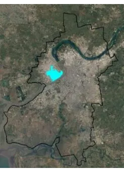
analysis zones (TAZ) are delineated on the basis of current ward boundaries which also acts as administrative boundaries for the purpose of elections. Indirectly TAZ are wards lying in the western zone of Surat city.
3. Selecting sample size and designing household questionnaire: a sample size of 344 households (10% of the total households in the study areas) [sample survey is based on the guidelines prescribed by the [8]] are taken for the analysis and preparing model for trip generation.
4. Collecting the required data: door to door survey is carried out to perform this exercise. Member from each households are inquired about the number of trips made each day, size of household, earning members in household, students in household, monthly expenditure etc.
5. Analysing data: the data collected is put into SPSS and trips produced on one axis is compared with different factors are such as monthly expenditure, family size etc. on other axis.
6. Building model: this includes estimation of feasible models for the total number of trips produced by the household, and the total number of trips for each category of home based trips utilizing multiple regression method.[9]
IV. DATA ANALYSIS AND RESULTS
For the purpose of data analysis, the survey data is fetched into excel and various components on which trip generation relies are selected first from the survey. After this, the number of household members, total employed persons in household, number of students in a family and monthly household income is compared corresponding to the number of trips generated. Various statistical functions are performed to commute the coefficient of relation between trips and others such as household size, number of employed persons in a household, number of students and monthly household income. The graph given below represents the relationship between number of trips vs. household size.
Figure 1. TAZ of the Study area
As can be inferred from the slope of the best fit line that the relation between trips generated and the Household size is significant. With increase in the family size the average number of trips also increases. The number of trips for family size 8 or beyond show very less trips thereby indicating few flaws in the process of household surveys. The graph given below represents the relationship between number of trips vs. vehicle ownership.
In the above graph the best fit line indicates a fair relationship between trips and the number of vehicles owned by the family i.e. increase in the number of vehicles corresponds to higher number of trips made by family. The graph represents the relationship between number of trips vs. monthly household income.
y = 0.593x + 1.532 R² = 0.190
0 2 4 6 8 10 12
0 2 4 6 8 10
T O TAL T R IP S
TOTAL HH MEMBER
T R I PS V S H H S I Z E
Figure 3. Trips vs. Household Size
Figure 4. Trips vs. Vehicle ownership
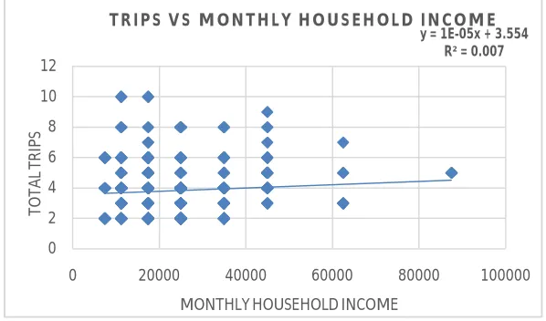
Figure 5. Trips vs. Monthly household income
y = 0.630x + 2.583 R² = 0.168
0 2 4 6 8 10 12
0 1 2 3 4 5 6 7 8
T O TAL T R IP S
NO. OF VEHICLES
T R I P S V S V E H I C L E O W N E R S H I P
y = 1E-05x + 3.554 R² = 0.007
0 2 4 6 8 10 12
0 20000 40000 60000 80000 100000
T O T AL T R IP S
MONTHLY HOUSEHOLD INCOME
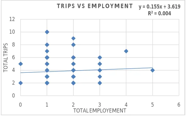
In earlier cases trips are fairly affected by the vehicle ownership and household size while in this case relation between trips and monthly household income isn’t high or in other words not highly correlated. The slope of best fit is very low thereby indicating low relationship between trips and monthly household income. Other socio economic factors such as number of students in a family when correlated with the number of trip per family comes out to be weak on a similar pattern, relation between trips and the number of the people employed in a family is also very weak. The graph given below represents the relationship between number of trips vs. employment.
The correlation coefficients of various factors is given in the table below.
Table 1. Factors and Correlation Coefficient.
As can be seen in the table that all the coefficients of correlation are positive in nature thereby indicating the increase in the number of trips for any increase in any of these factors. As can also be observed that the number of members in a family is highly related to the number of trips generated by the Household followed by the number of the vehicles owned by the household. The lowest correlation coefficient is of employment i.e. number of people employed in a family. The same can be observed in the graphs between trips and other factors taken for the estimating the future trip generation or for the modelling purpose.
FACTORS CORRELATION
COEFFICIENTS
HOUSEHOLD SIZE 0.436967176
MONTHLY HOUSEHOLD INCOME
0.08409733
EMPLOYMENT 0.063498759
VEHICLE OWNERSHIP 0.410307899
Figure 6. Trips vs. Employment
y = 0.155x + 3.619 R² = 0.004
0 2 4 6 8 10 12
0 1 2 3 4 5 6
T
O
T
AL
T
R
IP
S
NUMBER OF TRIPS GENERATED= 0.437*XHH+0.063*XE+0.084*XI+0.410*XVO
XHH: Number of household members
XE: Number of persons employed in a family
XI: Household income
XVO: Number of vehicles owned
V. TESTING GOODNESS OF FIT: R2
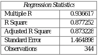
The regression statistics is represented in the table given below.
Table 2. Regression Statistics
Goodness of fit basically indicates the applicability of the model, in our case goodness of fit comes out to be 87% i.e. means the factors taken for deciding the trips generated in the future are valid and plays an important role while commuting the future trip generation rate. A better results can be obtained if some more factors can be assessed to calculate the trip generation in future. But as per many studies[10][9] a goodness of fit as high as 0.87 indicates the applicability of the model on the realistic world working projects.
VI. CONCLUSION
In this study the key determinants affecting the trip making rates such as family income, number of members in a family, vehicles owned by the family, number of persons employed in a family are seen at a household level for the western part of Surat city. Using multiple regression model, the results that are generated showed high dependency of trip making on the factors looked upon on household level. High value of goodness of fit indicates that the model is well defined and the trips are a function of the variables chosen for this study. Surat in today’s time is in transition stage from a medium size city to a large metropolis, eventually the number of trips are also increasing drastically. Such models can be used for providing a public transport designed for higher ridership along with the comfort equivalent to that of private mode of transport. High usage of public transport system for any city located in any part of the world eventually helps in achieving less carbon emission goals set up by the governments not only in India but around the world. Not limited to the reduction of carbon emissions, shift to public transport can also be useful in lowering the burden on the roads and flyovers in the city of Surat. Information of the future trips can also be used for designing the roads with highest possible level of service and it can also be used for implementation of the Travel Demand Management measures such as road pricing, park and ride facilities and many more. Route of Bus Rapid Transit System can be planned based on these calculations for optimum ridership in the transit facility.
REFERENCES
[1] Embarq, “transport in cities:india indicators,” Centere for sustainable trasnport, mumbai, 2011.
[2] R. p. vijay kumar, “Reforms in Urban Planning and Development Process: Case of,” International Journal of Engineering Inventions, pp.
75-82, 2013.
[3] NPTEL, “Trip generation,” in Introduction to Transportation Engineering , mumbai, 2007, pp. 7.1-7.5.
Regression Statistics
Multiple R 0.936617
R Square 0.877252
Adjusted R Square 0.873228
Standard Error 1.464898
[4] G. P. HJ Wootton, “A MODEL FOR TRIPS GENERATED BY HOUSEHOLD,” JOURNAL OF TRANSPORT ECONOMICS AND POLICY, pp. 137-153, 1967.
[5] P. R. a. G. Floater, “ACCESSIBILITY IN CITIES:TRANSPORT AND URBAN FORM,” NCE Cities – Paper 03, pp. 1-60, 2015.
[6] S. S. K. G. J. K. Navya S V., “TRIP GENERATION MODEL FOR THE CORE AREA OF,” International Journal of Innovative Research
in Science, Engineering and Technology, pp. 99-106, December 2013 .
[7] M. D, “Household and Travel Characterstics in two middle income residential colonies of Delhi,” Traffic and Road research laboratory
supplementary report, delhi, 1986.
[8] WILBUR SMITH ASSOCIATES, “study on traffic and trasnportation policies and strategies in urban areas in india,” Ministry of Urban
Development, India, DELHI, may 2008.
[9] A. M. Y. Dodeen, “Developing trip generation models : utilizing linear regression analayis :jericho city as case study,” faculty of
Graduate studies, An-Najah National University, 2014.
[10] F. A. W. A. Colin Cameron, “An R-squared measure of goodness of fit for some common nonlinear regression models,” pp. 16-32, 1995.