Parameter Identification for Dispersive Dielectrics Using
Pulsed Microwave Interrogating Signals and Acoustic Wave
Induced Reflections in Two and Three Dimensions
H. T. Banks
†and V. A. Bokil
‡Center for Research in Scientific Computation
North Carolina State University
Raleigh, N.C. 27695-8205
Abstract
In this report we consider an electromagnetic interrogation technique for identifying the dielectric parameters of a Debye medium in two and three dimensions. These parameters include the dielectric permittivity, the conductivity and the relaxation time of the Debye medium. In this technique a travelling acoustic pressure wave that is generated in the Debye medium is used as a virtual reflector for an interrogating microwave electromagnetic pulse that is generated in free space and impinges on a planar interface that separates air and the Debye medium. The reflections of the microwave pulse from the air-Debye interface and from the acoustic pressure wave are recorded at an antenna that is located in air. These reflections comprise the data that is used in an inverse problem to estimate the dielectric parameters of the Debye medium. We assume that the dielectric parameters of the Debye medium are locally pressure dependent. A model for acoustic pressure dependence of the material constitutive parameters in Maxwell’s equations is presented. As a first approximation, we assume that the Debye dielectric parameters are affine functions of pressure. We present a time domain formulation that is solved using finite differences in time and in space using the finite difference time domain method (FDTD). Perfectly matched layer (PML) absorbing boundary conditions are used to absorb outgoing waves at the finite boundaries of the computational domain and prevent excessive spurious reflections from reentering the domain and contaminating the data that is collected at the antenna placed in air.
1
Introduction
The study of transient electromagetic waves in lossy dispersive dielectrics is of great interest due to the numerous applications of this subject to many different problems [AMP94, APM89]. These include microwave imaging for medical applications in which one seeks to investigate the internal structure of an object (the human body) by means of electromagnetic fields at microwave frequencies (300 MHz - 30 GHz). This is done for example, to detect cancer or other anomalies by studying changes in the electrical properties of tissues [FMS03]. These include the dielectric properties such as permittivity, the conductivity and the relaxation time for the Debye medium. One generates the electrical property distributions in the body (Microwave maps) with the hope that such properties of different bodily tissues are related to their physiological state. With such noninvasive interrogating techniques one can study properties and defects in biological tissues with very little discomfort to the subjects. Other potential applications for such interrogation techniques are nondestructive damage detection in aircraft and spacecraft where very high frequency electromagnetic pulses can be used to detect the location and width of any cracks that may be present [BGW03]. Additional applications are found in mine, ordinance and camouflage surveillance, and subsurface and atmospheric environmental modeling [BBL00].
Another important technique employed in noninvasive interrogation of objects is the use of ultrasonic waves in industrial and medical applications. The interaction of electromagnetic and sound waves in matter has been widely studied in acoustooptics [And67, Kor97]. Brillouin first showed that electromagnetic and sound waves can interact in a medium and influence each others propagation dynamics [Bri60]. The response of the atomic electrons in a material medium to the applied electric field results in a polarization of the material with a resulting index of refraction that is a function of the density in the material. Consequently, the material density fluctua-tions produced by a sound wave induce perturbafluctua-tions in the index of refraction. Thus an electromagnetic wave transmitted through the medium will be modulated by the sound wave, and scattering and reflection will occur. Conversely, a spatial variation of the electromagnetic field intensity and the corresponding electromagnetic stress lead to a volume force distribution in the medium. This is called electrostriction, and can lead to sound generation. This mutual interaction between light and sound may also lead to instabilities and wave amplification [MI68].
terrogation problem is presented for dispersive media backed by perfect conductor walls and the FDTD method is utilized [Taf95, Taf98]. However, as we have noted above, the object of interrogation may not be backed by perfect conductor walls in many important applications, and hence one needs to have another type of accessible interface which will reflect the propagating electromagnetic pulses. It is therefore of great importance to ascertain (computationally and experimentally) whether the interrogation ideas of [ABR02] using acoustic pressure waves as virtual reflectors can be effective in multidimensional settings. The goal of this paper is the investigation of computational and statistical aspects of this methodology. At present we are also trying to validate these proposed techniques by testing the ideas in this paper in an experimental setup. Our group has built an antenna that we are using to study the acoustooptical interaction in agar-agar in which the sound waves are produced by means of a transducer [ABK04]. In such a setup, as well as in many applications one cannot assume normally incident plane waves impinging on the agar, and hence one needs to consider the more general case of oblique incidence. This motivates the study of an electromagnetic interrogation technique using the acoustooptical interaction to study dielectic properties of dispersive media in multidimensions.
We begin with Maxwell’s equations for a first order dispersive (Debye) media with Ohmic conductivity and incorporate a model that describes the electromag-netic/acoustic interaction. Our model features modulation of the material polariza-tion by the pressure wave and thus the behaviour of the electromagnetic pulse. This approach is based on ideas found in [MI68]. We incorporate a pressure dependent Debye model for orientational polarization into Maxwell’s equations. We model the propagation of a non-harmonic pulse from a finite antenna source in free space im-pinging obliquely on a planar interface into the Debye medium. We use the finite difference time domain method (FDTD) [Taf95] to discretize Maxwell’s equations and to compute the components of the electric field in the case where the signal and the dielectric parameters are independent of the y variable. Figure 1 depicts the antenna and the Debye dielectric slab geometry that we will model in our problem with the infinite dielectric slab perpendicular to the z-axis and uniform in the y -direction and finite in the x-direction lying in the region−∞ ≤y≤ ∞, x1 ≤x≤x2.
An alternating current along the x-direction of the antenna located at z = zc then produces an electric field that is uniform in y with nontrivial components Ex and Ez depending on (t, x, z). When propagated in the xz-plane, this results in oblique incident waves on the dielectric surface in the xy-plane at z = z1. (In [BF95] the
authors use Fourier-series in the frequency domain to compute the propagation of a time harmonic pulse train of plane waves that enter a dielectric across a planar boundary at oblique incidence. They showed that precursors are excited by short rise time pulses at oblique incidence. However, the use of Fourier series restricts this approach to harmonic pulses.) The oblique waves impinge on the planar inter-face that separates air and the Debye medium at z =z1 where they undergo partial
z =zc and is recorded. The transmitted part of the wave travels through the Debye medium and intercepts an acoustic pressure wave that is generated in the dielectric medium. Here the microwave pulse undergoes partial transmission and reflection. The reflected wave travels back through the Debye medium, undergoes a secondary reflection/transmission at the air-Debye interface and is then recorded at the antenna. Thus the antenna records three pieces of information; the input source, the reflection of the electromagnetic pulse from the air-Debye interface and the reflection from the pressure wave region. This data is recorded at the center of the antenna and will be used in an inverse problem to estimate the dielectric properties of the Debye medium. We note that the acoustic wave speed is many orders of magnitude smaller than the speed of light. Thus the acoustic pressure wave is almost stationary relative to the microwave pulse. In this report, we have assumed that the acoustic pressure wave is specified a priori and hence we assume that the pressure wave is not modified by the electromagnetic wave. This leads to a much simplified electromagnetic/acoustic interaction model. The dynamic interaction between the two and the appropriateness of this simplifying assumption are currently being investigated and will be the topic of a future report.
An important computational issue in modeling two or three dimensional wave propagation is the construction of a finite computational domain and appropriate boundary conditions for terminating this domain in order to numerically simulate an essentially unbounded domain problem. We surround the domain of interest by perfectly matched absorbing layers (PML’s), thus producing a finite computational domain. The original PML formulation is due to J. P. Berenger [Ber94] and was based on a split form of Maxwell’s equations in which all the fields themselves were split into orthogonal subcomponents. This formulation was appropriately called the split field form. Many different variations of the split field PML are now available in the literature. Most of these different formulations, though equivalent to the split field PML, do not involve the splitting of the fields or splitting of Maxwell’s equations. The PML formulation that we use in this report is based on the anisotropic (uniaxial) formulation that was first proposed by Sacks et. al. [SKLL95].
We first present numerical results for the forward problem for two different test cases. The relaxation times of the Debye media in these two test cases differ by many orders of magnitude. We perform a sensitivity analysis in each test case to determine which parameters are most likely to be accurately estimated in an inverse problem. We also determine which of the pressure dependent parameters are the most significant in each of the test cases. As we shall see, the significant difference in the orders of magnitude of the relaxation times for the two test cases produces inverse problems with very different estimation properties.
method, which is a gradient based algorithm, and the Nelder-Mead method, which is based on simplices and is gradient free. For the first test case, these two algorithms produce similar results. However, in the second test case, we see the presence of many local minima and the Nelder-Mead algorithm converges to a local minima instead of the global minimum.
We also consider uncertainty in estimates due to data uncertainty. We present a model for generating noisy data that we use in our inverse problems to simulate experimental settings in which noise enters into the problem in a natural fashion. We then discuss a statistical error methodology to analyze the results of the inverse prob-lems based on noisy data. This statistical error analysis is used to obtain confidence intervals for all the parameters estimated in the inverse problem. These intervals indicate the level of confidence that can be associated with estimates obtained with our methodology.
2
Model formulation: The forward problem
We consider Maxwell’s equations which govern the electric fieldE and the magnetic field H in a domain Ω with charge densityρ. Thus we consider the system
(i) ∂D
∂t +J− ∇ ×H= 0, in (0, T)×Ω,
(ii) ∂B
∂t +∇ ×E= 0, in (0, T)×Ω, (iii) ∇ ·D=ρ, in (0, T)×Ω,
(iv) ∇ ·B= 0, in (0, T)×Ω,
(v) E×n= 0, on (0, T)×∂Ω,
(vi) E(0,x) = 0, H(0,x) = 0, in Ω.
(1)
The fields D,B are the electric and magnetic flux densities respectively. All the fields in (1) are functions of position r = (x, y, z) and time t. We have J = Jc+Js, where Jc is a conduction current density and Js is the source current density. We assume only free space (actually the antenna in our example) can have a source current, and Jc is only found in the dielectric material. The condition (1, v) is a perfectly conducting boundary condition on the computational domain which we will replace with absorbing conditions in the sequel. With perfect conductor conditions, the computational boundary acts like a hard wall to impinging electromagnetic waves causing spurious reflections that would contaminate the data that we wish to use in our inverse problems.
Constitutive relations which relate the electric and magnetic fluxes D,B and the electric currentJcto the electric and magnetic fieldsE,Hare added to these equations
electromagnetic fields. In free space, these constitutive relations are D = 0E, and B = µ0H, where 0 and µ0 are the permittivity and the permeability of free space,
respectively, and are constant [Jac99]. In general there are different possible forms for these constitutive relationships. In a frequency domain formulation of Maxwell’s equations, these are usually converted to linear relationships between the dependent and independent quantities with frequency dependent coefficient parameters. We will consider the case of a dielectric in which magnetic effects are negligible, and we assume that Ohm’s law governs the electric conductivity. Thus, within the dielectric medium we have constitutive relations that relate the flux densities D,B to the electric and magnetic fields, respectively. We have
(i) D =0E+PID,
(ii) B =µ0H,
(iii) Jc =σEID,
(2)
In (2), ID denotes the indicator function on the Debye medium. Thus, Jc = 0 in air. The quantity P is called the electric polarization. It is equal to zero in air and is nonzero in the dielectric. Electric polarization may be defined as the electric field induced disturbance of the charge distribution in a region. This polarization may have an instantaneous component as well as ones that do not occur instantaneously; the latter usually have associated time constants called the relaxation times which are denoted by τ. We let the instantaneous component of the polarization to be related to the electric field by means of a dielectric constant 0χ and denote the remainder
of the electric polarization as PR. We have
P=PI+PR =0χE+PR, (3)
and hence the constitutive law (2, i) becomes
D=0rE+PR, (4)
where r = (1 +χ) is the relative permittivity of the dielectric medium.
To describe the behaviour of the media’s macroscopic electric polarization PR,
we employ a general integral equation model in which the polarization explicitly de-pends on the past history of the electric field. This model is sufficiently general to include microscopic polarization mechanisms such as dipole or orientational polariza-tion(Debye), as well as ionic and electronic polarization(Lorentz), and other frequency dependent polarization mechanisms [And67] as well as multiples of such mechanisms represented by a distribution of the associated time constants (e.g., see [BG04]). The resulting constitutive law can be given in terms of a polarization or displacement susceptibility kernel g as
1
z1 z
x
y
E(t,x,z)
Figure 1: Antenna and dielectric slab configuration.
which, in the case (Debye) of interest to us here, can be written as
g(t) = e−t/τ0(s−∞)
τ . (6)
Such a Debye model can be represented in differential form as
τP˙R+PR =0(s−∞)E,
D =0∞E+PR,
(7)
inside the dielectric, whereas PR = 0, ∞ = 1 in air, and ∞ = r in the dielectric. We will henceforth denote PR by P. In equations (5) and (7), the parameters s and ∞ denote the static relative permittivity, and the value of permittivity for an
extremely high(≈ ∞) frequency field, respectively. The quantity∞ is called the
infi-nite frequency permittivity. Biological cells and tissues display very high values of the dielectric constants at low frequencies, and these values decrease in almost distinct steps as the excitation frequency is increased. This frequency dependence of permit-tivity is called dielectric dispersion and permits identification and investigation of a number of completely different underlying mechanisms. This property of dielectric materials makes the problem of parameter identification an important as well as very useful topic for investigation.
We will modify system (1) and the constitutive laws (2) by performing a change of variables that renders the system in a form that is convenient for analysis and computation. From (1, i) we have
∂ ∂t
D+
Z t
Jc(s,x) ds
Next, we define the new variable
e
D(t,x) =D(t,x) +
Z t
0
Jc(s,x) ds. (9)
Using definition (9) in (8) and (1) we obtain the modified system
(i) ∂De
∂t − ∇×H=−Js in (0, T)×Ω,
(ii) ∂B
∂t +∇×E= 0 in (0, T)×Ω, (iii) ∇ ·De = 0 in (0, T)×Ω,
(iv) ∇ ·B= 0 in (0, T)×Ω,
(v) E×n= 0 on (0, T)×∂Ω,
(vi) E(0,x) = 0, H(0,x) = 0 in Ω.
(10)
We will henceforth drop the ˜ symbol on D. We note that equation (10, iii) follows from the continuity equation ∂ρ∂t +∇ ·J = 0, the assumption that ρ(0) = 0, and the assumption that∇ ·Js = 0 (in the sense of distributions). The modified constitutive laws (2) after substitution of Ohm’s law and (9) are
(i) D(t,x) = 0∞(x)E(t,x) +PR+
Z t
0
σ(x)E(s,x) ds,
(ii) B =µ0H,
(11)
with PR, the solution of
τP˙R+PR =0(s−∞)E. (12)
3
An anisotropic perfectly matched layer
absorb-ing medium
to free space and then we will explain how this construction can be generalized to the case of a Debye medium.
The source current Js is zero inside the PML regions. So we will neglect Js in this section. We model the PMLs as lossy regions by adding artificial loss terms to Maxwell’s equations. This approach is based on using anisotropic material properties to describe the absorbing layer [SKLL95, Ged96, Rap95]. We start with Maxwell’s equations in the most general form
∂D
∂t =∇×H−Je, ∂B
∂t =−∇×E−Jm,
∇ ·D = 0,
∇ ·B = 0,
(13)
where Je and Jm are electric and magnetic conductivities, respectively. Inside the computational domain we will have Je = Jc and Jm = 0. We will derive a PML model in the frequency domain and then transform the corresponding equations to the time domain by taking the inverse Fourier transforms of the frequency domain equations. To this end, we consider the time-harmonic form of Maxwell’s equations (13) given by
jωDˆ =∇×Hˆ −ˆJe,
jωBˆ =−∇×Eˆ −Jˆm,
∇ ·Bˆ = 0,
∇ ·Dˆ = 0,
(14)
where for every field vector V, ˆV denotes its Fourier transform. We then have the
constitutive laws
ˆ
B= [µ] ˆH,
ˆ
D= [] ˆE,
ˆ
Jm = [σM] ˆH,
ˆ
Je = [σE] ˆE.
(15)
In (15) the square brackets indicate a tensor quantity. Thus we allow for anisotropy in our media by permitting the material parameters to be tensors. Note that when the density of electric and magnetic charge carriers in the medium is uniform throughout space, then ∇ ·Jˆe = 0 and∇ ·Jˆm = 0. We define the new tensors
[¯µ] = [µ] + [σM] jω ,
[¯] = [] + [σE] jω .
Using the definitions (16) we define two new constitutive laws that are equivalent to (15), given by
ˆ
Bnew= [¯µ] ˆH,
ˆ
Dnew= [¯] ˆE.
(17)
Using (17) in (14), we can write Maxwell’s equations in time-harmonic form as
jωDˆnew =∇×Hˆ,
jωBˆnew =−∇×Eˆ,
∇ ·Dˆnew = 0,
∇ ·Bˆnew = 0.
(18)
The split-field PML introduced by Berenger [Ber94] is a hypothetical medium based on a mathematical model. In [MP95] Mittra and Pekel showed that Berenger’s PML was equivalent to Maxwell’s equations with a diagonally anisotropic tensor appearing in the constitutive relations for D and B. For a single interface, the anisotropic medium is uniaxial and is composed of both the electric and magnetic permittivity tensors. This uniaxial PML (UPML) formulation performs as well as the original split-field PML while avoiding the nonphysical field splitting. As will be shown below, by properly defining a general constitutive tensor [S], we can use the UPML in the interior working volume as well as the absorbing layer. This tensor provides a lossless isotropic medium in the primary computation zone, and individual UPML absorbers adjacent to the outer lattice boundary planes for mitigation of spurious wave reflections. The fields excited within the UPML are also plane wave in nature and satisfy Maxwell’s curl equations. The derivation of the PML properties of the tensor constitutive laws is also done directly by Sacks et al. in [SKLL95] and by Gedney in [Ged96]. We follow the derivation by Sacks et al. here. We begin by considering planar electromagnetic waves in free space incident upon a PML half space. Starting with the impedance matching assumption, i.e., the impedance of the layer must match that of free space: −1
0 µ0 = [¯]−1[¯µ] we have
[¯] 0
= [¯µ] µ0
= [S] = diag{a1, a1, a3}. (19)
Hence, the constitutive parameters inside the PML layer are [¯] = 0[S] and [¯µ] =
µ0[S], where [S] is a diagonal tensor. We next consider plane wave solutions of the
form
V(x, t) = ˆV(x) exp(j(ωt−k·x)), (20)
to be
k2
x a2a3
+ k
2
y a1a3
+ k
2
z a1a2
=k20 ≡ω2µ00 ≡
ω2
c2 0
. (21)
where, c0 is the speed of light in free space.
To further explain our UPML formulation, we may, without loss of generality, consider a PML layer which fills the positive xhalf-space and plane waves with wave vectors in the xz- plane (ky = 0). Let θi be the angle of incidence of the plane wave measured from the normal to the surface x= 0. The standard phase and magnitude matching arguments at the interface yield the following generalization of Snell’s law
√
a1a3sinθt= sinθi, (22)
whereθtis the angle of the transmitted plane wave. Matching the magnitudes of the electric and magnetic fields at the interface, x= 0, we obtain the following values of the reflection coefficients for the TE and the TM modes
RT E =
cosθi −
r
a3
a2
cosθt
cosθi+
r
a3
a2
cosθt
RT M =
r
a3
a2
cosθt−cosθi
cosθi+
r
a3
a2
cosθt
(23)
From (23) we can see, that by choosing a3 = a2 = a and √a1a3 = 1, the interface
is completely reflectionless for any frequency, angle of incidence, and polarization. Using (17) and (19), we thus find the constitutive laws for the perfectly matched
layer are
ˆ
Dnew = 0[S] ˆE,
ˆ
Bnew = µ0[S] ˆH,
(24)
where the tensor [S] is
[S] =
a−1 0 0
0 a 0
0 0 a
. (25)
The perfectly matched layer is therefore characterized by the single complex number a. Taking it to be the constant a = γ −jβ, and substituting into the dispersion relation (21), we obtain the following expression for the electric field inside of the PML
ˆ
E(x, y, z) = ˆE0exp(−k0βcosθtx) exp(−jk0(γcosθtx+ sinθtz)) exp(jωt). (26)
Remark 1 To match the anisotropic PML along a planar boundary to a dispersive isotropic half-space, we will need to modify the above construction for the phasor-domain constitutive relation
ˆ
D=0r(ω)Eˆ, (27)
where r(ω) is the frequency dependent relative permittivity of the Debye medium, which will be defined in a standard manner in (40) below.
3.1
Implementation of the uniaxial PML
To apply the perfectly matched layer to electromagnetic computations, we replace the half infinite layer by a layer of finite depth backed with a more conventional boundary condition, such as a perfect electric conductor (PEC). This truncation of the layer will lead to reflections generated at the PEC surface, which can propagate back through the layer to re-enter the computational region. In this case, the reflection coefficient R, is now a function of the angle of incidence θ, the depth of the PML δ, as well as the parameter a in (25). Thus, this parameter a for the PML is chosen in order for the attenuation of waves in the PML to be sufficient so that the waves striking the PEC surface are negligible in magnitude. Perfectly matched layers are then placed near each edge (or face in the 3D case) of the computational domain where a non-reflecting condition is desired. This leads to overlapping PML regions in the corners of the domain. As shown in [SKLL95], the correct form of the tensor which appears in the constitutive laws for these regions is the product
[S] = [S]x[S]y[S]z, (28)
where component [S]α in the product (28) is responsible for attenuation in the α direction, for α = x, y, z (see Figure 2). All three of the component tensors in (28) are diagonal and have the forms
[S]x =
s−1
x 0 0
0 sx 0
0 0 sx
; [S]y =
sy 0 0
0 s−1
y 0
0 0 sy
; [S]z =
sz 0 0
0 sz 0
0 0 s−1
z
. (29)
In the above sx, sy, sz are analogous to the complex valued parametera encountered in the Section 3 analysis of the single PML layer. Thus,sα governs the attenuation of the electromagnetic waves in the α direction for α =x, y, z. When designing PML’s for implementation, it is important to choose the parameters sα so that the resulting frequency domain equations can be easily converted back into the time domain. The simplest of these [Ged96] which we employ here, is
Working Volume
[S] = [S]z
6
?
[S] = [S]x
PML PEC WALL
?
Corner Region
?
6
? 6 ? 6 ?
σx = 0 σx >0
σx >0
-σz = 0 σz >0
σz >0
@ @
@ R
Figure 2: PML layers surrounding the domain of interest. In the corner regions of the PML, both σx and σz are positive and the tensor [S] is the product [S]x[S]z. In the remaining regions only one ofσz (left and right PML’s) orσx (top and bottom PML’s) are nonzero and positive. The tensor [S], is thus either [S]x or [S]z respectively. The PML is truncated by a perfect electric conductor (PEC).
The PML interface represents a discontinuity in the conductivities σα. To reduce the numerical reflections caused by these discontinuous conductivities, the σα are chosen to be functions of the variable α (e.g., σx is taken to be a function of x in the [S]x component of the PML tensor). A choice of these functions so that σα = 0, i.e., sα = 1 at the interface yields the PML a continuous extension of the medium being matched and reduces numerical reflections at the interface. If one increases the value of σα with depth in the layer, one obtains greater overall attenuation while minimizing the numerical reflections. Gedney [Ged96] suggests a conductivity profile
σα(α) = σmax|α−α0| m
δm ; α =x, y, z. (31)
where δ is the depth of the layer, α = α0 is the interface between the PML and
the computational domain, and m is the order of the polynomial variation. Gedney remarks that values of m between 3 and 4 are believed to be optimal. For the conductivity profile (31), the PML parameters can be determined for given values of m, δ, and the desired reflection coefficient at normal incidenceR0, as
σmax ≈
(m+ 1) ln(1/R0)
2ηIδ
, (32)
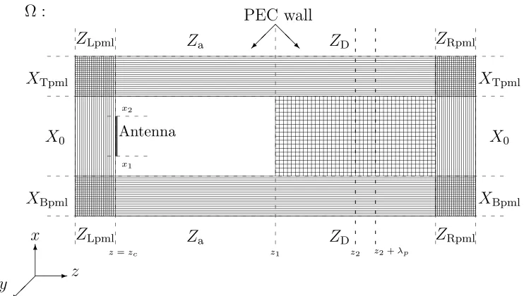
z1 z2 z2+λp
ZRpml
ZRpml
Ω :
z=zc
ZLpml Za ZD
ZLpml Za ZD
XBpml
X0
XTpml
XBpml
X0
XTpml
x1
x2
Antenna
x
z y
6
-@ @ R
PEC wall
Figure 3: PML layers surrounding the domain of interest.
that, for a broad range of problems, an optimal value of σmax is given by
σopt ≈
m+ 1 150π∆α√r
, (33)
where ∆α is the space increment in the αdirection and r is the relative permittivity of the material being modeled. In the case of free space r = 1. Since we desire to match the PML to both free space as well as the Debye medium, we will user to be the average value
r = 1
2(1 +∞). (34)
3.2
Reduction to two dimensions
From the time-harmonic Maxwell’s curl equations in the PML (18) and (24), Ampere’s and Faraday’s laws can be written in the most general form as
jωµ0[S]Hˆ =−∇×Eˆ, (Faraday’s Law)
jω[S]Dˆ =∇×Hˆ −Js, (Ampere’s Law) (35)
intervals asX =XBpml∪X0∪XTpml and the interval Z into disjoint closed intervals
asZLpml∪Za∪ZD∪ZRpml, as seen in Figure 3. The computational domain of interest
is the region X0 × {Za∪ZD}, where X0×Za denotes air and X0×ZD denotes the
Debye medium. The buffer region D \ (X0 × {Za ∪ZD}) contains the absorbing
layers (PML’s). The PML’s are backed by a perfect conductor where the boundary condition n × E = 0 is used. We construct perfectly matched layers in regions where (x, z) ∈ (XBpml ∪XTpml) ×(ZLpml ∪ZRpml). To obtain a two-dimensional
model, we make the assumption that the signal and the dielectric parameters are independent of the y variable. Also, an alternating current along the x direction, as in (54), then produces an electric field that is uniform inywith nontrivial components Ex and Ez depending on (t, x, z) which, when propagated in the xz plane result in oblique incident waves on the dielectric surface in thexy plane atz =zc. With these assumptions, Maxwell’s equations reduces to a two dimensional system for solutions involving the Ex and Ez components for the electric field and the component Hy for the magnetic field, which is refered to as the TEy mode. In this case, we haveσy = 0 and sy = 1 in the UPML. From (11, i) and (7) expressed in the frequency domain we have the constitutive relation
ˆ
D=0
∞+
s−∞
1 + jωτ + σ jω0
E. (36)
Rescaling the electric field as
˜ ˆ E = r 0 µ0 ˆ
E, (37)
we can write the time-harmonic frequency domain Maxwell’s equations (35) in the uniaxial medium as
(i) jω
1 + σz(z) jω0
1 + σx(x) jω0
−1
ˆ˜
Dx =−c0(
∂Hˆy
∂z +Js·xˆ),
(ii) jω
1 + σx(x) jω0
1 + σz(z) jω0
−1
ˆ˜ Dz =c0
∂Hˆy ∂x ,
(iii) jω
1 + σx(x) jω0
1 + σz(z) jω0
ˆ Hy =c0
∂Eˆz
∂x −
∂Eˆx ∂z
!
.
(38)
In the above c0 = 3.0×10⁸ m/s is the speed of light in vacuum and ˆ˜D = ( ˆ˜Dx,Dˆ˜z)T is defined as
ˆ˜
D=∗r·Eˆ˜, (39)
with
∗
r =∞+
s−∞
1 + jωτ + σ jω0
. (40)
To this end, we introduce the fields ˆ D∗
x =s−x1Dˆ˜x,
ˆ D∗
z =s
−1
z Dˆ˜z,
ˆ H∗
y =szHˆy.
(41)
Again, dropping the˜symbol onD and transforming the frequency domain equations to the time domain, we obtain the system
(i) ∂tHy∗ + σx(x)
0
H∗
y =c0
∂Ez ∂x − ∂Ex ∂z ,
(ii) ∂tHy+ σz(z)
0
Hy =∂tHy∗,
(iii) ∂tDx∗+ σz(z)
0
D∗
x=−c0(
∂Hy
∂z +Js·ˆx),
(iv) ∂tDx =∂tD∗x+ σx(x)
0
D∗
x,
(v) ∂tDz∗+ σx(x)
0
D∗
z =c0
∂Hy ∂x ,
(vi) ∂tDz =∂tDz∗+ σz(z)
0
D∗
z,
(42)
with
D(t) =∞E(t) +P(t) +C(t), (43)
where D = (Dx, Dz)T, and inside of the dielectric the polarization P = (Px, Pz)T satisfies
τP˙ +P= (s−∞)E, (44)
while the conductivity term C= (Cx, Cy)T satisfies
˙
C= (σ/0)E . (45)
inside of the dielectric. Outside the dielectric we have P= C= 0. We will assume zero initial conditions for all the fields.
3.3
Pressure dependence of polarization
We suppose as a first approximation that each of the pressure dependent parameters can be prepresented as a mean value plus a perturbation that is proportional to the
pressure
(i) τ(p) =τ0+κτp,
(ii) s(p) =s,0+κsp,
(iii) ∞(p) =∞,0+κ∞p.
(47)
This can be considered as a truncation after the first-order terms of power series expansion of these functions of p. Thus (44) is written as
(τ0+κτp) ˙P+P= ((s,0−∞,0) + (κs−κ∞)p)E. (48)
This model features modulation of the material polarization by the pressure wave and thus the behaviour of the electromagnetic pulse. We will assume that the acoustic pressure wave is specified a priori. The pressure pwill be assumed to have the form
p(t, z) =I(z2,z2+λp)sin
ωp[t+ z−z2 cp
]
, (49)
where z2 ∈ZD with z1 < z2. The termsωp, λp and cp denote the acoustic frequency, wavelength and speed respectively. We note that outside the pressure region, the pressure coefficients κτ, κs and κ∞ are all zero and
τ =τ0, s=s,0, ∞ =∞,0. (50)
From (43)
(i)(ii) DDx(t) = (∞,0+κ∞p)Ex(t) +Px(t) +Cx(t),
z(t) = (∞,0+κ∞p)Ez(t) +Pz(t) +Cz(t), (51)
with
(i)(ii) ((ττ0+κτp) ˙Px+Px = ((s,0−∞,0) + (κs−κ∞)p)Ex,
0+κτp) ˙Pz +Pz = ((s,0 −∞,0) + (κs−κ∞)p)Ez,
(52)
and
(i)(ii) CC˙˙x = (σ/0)Ex,
z = (σ/0)Ez.
(53)
3.4
Source term
in the y direction (see again Figure 1). We therefore take
Js(t, x, z) =I(x1,x2)(x)δ(z−zc) sin(ωc(t−3t0)) exp −
t−3t0
t0
2! ˆ x,
t0 =
2 ωd−ωc
, ωc = 2πfc rad/sec.
(54)
where I(x1,x2) is the indicator function on the interval (x1, x2) ∈ X0, δ(z − zc) is
the Dirac measure centered at z = zc, and ˆx is the unit vector in the x direction. The Fourier spectrum of this pulse has even symmetry about the frequency fc. The pulse is centered at time step 3t0 and has a 1/e characteristic decay of t0 time-steps
[Taf95]. We will specify the values of all the different quantities involved in (54) when we define the particular problems that we will solve. The source (54) radiates numerical waves having time waveforms corresponding to the source function. In the discretized model, described below the radiated numerical wave will propagate to the Debye medium and undergo partial transmission and partial reflection, and time stepping can be continued until all transients decay.
3.5
Space and time discretization
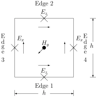
We will use the FDTD algorithm [Taf95] to discretize Maxwell’s equations. The FDTD algorithm uses forward differences to approximate the time and spatial deriva-tives. The FDTD technique rigorously enforces the vector field boundary conditions at interfaces of dissimilar media at the time scale of a small fraction of the impinging pulse width or carrier period. This approach is very general and permits accurate modeling of a broad variety of materials ranging from living human tissue to radar absorbers to optical glass. The system of equations (42) can be discretized on the stan-dard Yee lattice. The domain Ω is divided into square cells of length h= ∆x= ∆z, h being the spatial increment. The degrees of freedom on an element are shown in Figure 4. The electric field degrees of freedom are at the midpoints of edges of the squares and the magnetic degrees of freedom are at the centers of cells. The time interval over which time stepping is done is divided into subintervals of equal size using the time increment ∆t. We perform normal leapfrogging in time and the loss terms are averaged in time. This leads to an explicit time stepping scheme. In this case, a stability condition (CFL) has to be satisfied [Taf95] in order to obtain a well posed computational scheme. The time step ∆t and the spactial increment h for the FD-TD scheme in non-dispersive dielectics are related by the condition
ηCN=
c0∆t
h < 1
√
Ez Ez
Ex Ex
Hy
Edge 1 Edge 2
E d g e 3
E d g e 4
h
-h
? 6
@@
@ @
@@ @
@
-6 v 6
Figure 4: Degrees of freedom ofE and H on a rectangle.
media satisfy the stability restriction of the standard FD-TD scheme in nondispersive dielectrics. He has also shown that the extensions do not preserve the non-dissipative character of the standard FD-TD scheme. The extended difference systems are more dispersive than the standard FD-TD, and their accuracy depends strongly on how well the chosen timestep resolves the shortest timescale in the problem regardless of whether it is the incident pulse timescale, the medium relaxation timescale, or the medium resonance timescale.
For any field variableV, we use the notationVr
l,m =V(r∆t, lh, mh), wherer, l, m∈
Norr =r0±1/2, l=l0±1/2, m=m0±1/2, withr0, l0, m0 ∈N. With the degrees of
freedom as shown in Figure 4, the Maxwell curl equations are discretized as follows. Given the values of the electric field at timen∆t and the values of the magnetic field at time (n−1/2)∆t, we then evaluate the magnetic field at time (n+ 1/2)∆t and the electric field at time (n+ 1)∆t. We have for H∗
y =H∗
H∗|n+1/2
i+1/2,k+1/2−H ∗|n−1/2
i+1/2,k+1/2
∆t +
σx(i+ 1/2) 0
H∗|n+1/2
i+1/2,k+1/2+H ∗|n−1/2
i+1/2,k+1/2
2
!
=c0
Ez|ni+1,k+1/2 −Ez|ni,k+1/2 ∆x
!
−c0
Ex|ni+1/2,k+1−Ex|ni+1/2,k ∆z
!
.
Solving (56) for H∗
|ni+1+1//22,k+1/2 we have the update equation
H∗
|ni+1+1//22,k+1/2 =
20−σx(i+ 1/2)∆t
20+σx(i+ 1/2)∆t
H∗
|ni+1−1//22,k+1/2+
20c0∆t
20+σx(i+ 1/2)∆t
×
Ez|ni+1,k+1/2−Ez|ni,k+1/2
∆x −
Ex|ni+1/2,k+1−Ex|ni+1/2,k ∆z
!
.
(57)
Similarly we discretize the update equations for the other field variables in (42). The update equation forHy =H is
H|ni+1+1//22,k+1/2 =
20−σz(k+ 1/2)∆t
20+σz(k+ 1/2)∆t
H|ni+1−1//22,k+1/2
+
20
20+σz(k+ 1/2)∆t
×H∗
|ni+1+1//22,k+1/2−H ∗
|ni+1−1//22,k+1/2
.
(58)
The update equation forD∗
x is
D∗
x|ni+1+1/2,k =
20 −σz(k)∆t 20+σz(k)∆t
D∗
x|ni+1/2,k
−
20c0∆t
20 +σz(k)∆t
× Hy|
n+1/2
i+1/2,k+1/2−Hy|
n+1/2
i+1/2,k−1/2
∆z +J
n s,i+1/2,k
!
,
(59)
where the electromagnetic input source is chosen to have the formJns,i+1/2,k =Jn
s,i+1/2,kˆx. The update equation forDx is
Dx|ni+1+1/2,k =Dx|ni+1/2,k+
20 +σx(i+ 1/2)∆t
20
D∗
x|ni+1+1/2,k
+
20−σx(i+ 1/2)∆t
20
D∗
x|ni+1/2,k.
(60)
The update equation forD∗
z is
D∗
z|ni,k+1+1/2 =
20−σx(i)∆t
20+σx(i)∆t
D∗
z|ni,k+1/2
+
20c0∆t
20+σx(i)∆t
× Hy|
n+1/2
i+1/2,k+1/2−Hy|
n+1/2
i−1/2,k+1/2
∆x
!
.
(61)
Finally the update equation for Dz is
Dz|ni,k+1+1/2 =Dz|ni,k+1/2+
20+σz(k+ 1/2)∆t
20
D∗
z|ni,k+1+1/2
For the update ofEx andEz we will combine equations (51)-(53). From (53) we have the update for Cx and Cz as
Cx|n+1 =Cx|n+
σ∆t 20
(Ex|n+1+Ex|n),
Cz|n+1 =Cz|n+
σ∆t 20
(Ez|n+1+Ez|n).
(63)
From (52) we have the update forPx as
Px|n+1 =
1 + ∆t
2(τ0+κτpn+1)
−1
1− ∆t
2(τ0+κτpn)
Px|n
+
1 + ∆t
2(τ0+κτpn+1)
−1
∆t((s,0−∞,0) + (κs−κ∞)pn)
2(τ0+κτpn)
Ex|n
+
1 + ∆t
2(τ0+κτpn+1)
−1
∆t((s,0−∞,0) + (κs−κ∞)pn+1)
2(τ0+κτpn+1)
Ex|n+1. (64)
Similarly, from (52) we have the update for Pz as
Pz|n+1 =
1 + ∆t
2(τ0+κτpn+1)
−1
1− ∆t
2(τ0+κτpn)
Pz|n
+
1 + ∆t
2(τ0+κτpn+1)
−1
∆t((s,0−∞,0) + (κs−κ∞)pn)
2(τ0+κτpn)
Ez|n
+
1 + ∆t
2(τ0+κτpn+1)
−1
∆t((s,0−∞,0) + (κs−κ∞)pn+1)
2(τ0+κτpn+1)
Ez|n+1. (65)
From (51) we have
Ex|n+1 =
1
(∞,0+κ∞pn+1)
Dx|n+1−Px|n+1−Cx|n+1
. (66)
Substituting the update equations forPn+1
x and Cxn+1 in (66) we obtain an expression for En+1
x in terms of Exn, Dxn+1, Cxn and Pxn given by
F(pn+1) =
1 + ∆t
2(τ0+κτpn+1)
−1
∆t((s,0−∞,0) + (κs−κ∞)pn+1)
2(τ0+κτpn+1)
+ (∞,0+κ∞pn+1) +
σ∆t 20
Ex|n+1 =F(pn+1)−1
"
Dx|n+1−Cxn− σ∆t
20
Ex|n−
1 + ∆t
2(τ0+κτpn+1)
−1
×
1− ∆t
2(τ +κ pn)
Px|n+
∆t((s,0−∞,0) + (κs−κ∞)pn)
2(τ +κ pn)
Ex|n
whereDx|n+1 is calculated from (60). Thus, all the terms on the right side are known quantities, and we can use equation (67) to updateEx. Similarly the update equation for Ez is
Ez|n+1 =F(pn+1)−1
"
Dz|n+1−Czn− σ∆t
20
Ez|n−
1 + ∆t
2(τ0+κτpn+1)
−1
×
1− ∆t
2(τ0+κτpn)
Pz|n+
∆t((s,0−∞,0) + (κs−κ∞)pn)
2(τ0+κτpn)
Ez|n
, (68)
with F(pn+1) as defined in (67). As before, we calculate D
z|n+1 from (62). Hence all terms on the right hand side are known.
4
The forward problem for a Debye medium: First
test case
As discussed in Section 3.3 the pressure dependent parameters ∗
s, ∗∞, and τ
∗ are
represented as a mean value plus a perturbation that is proportional to the pressure in equations (47) (as discussed in [ABR02]). In our first test case, we present numerical simulations for a Debye medium that is similar to water. For signal bandwidths in the microwave regime the dispersive properties of pure water are usually modeled by a Debye equation having a single molecular relaxation term. The mean values ∗
s,0,
∗
∞,0, and τ0∗ for this Debye model [APM89] are given by
∗
s,0 = 80.1 (relative static permittivity),
∗
∞,0 = 5.5 (relative high frequency permittivity),
τ∗
0 = 8.1×10⁻¹² seconds,
σ∗ = 1
×10−5 mhos/meter,
(69)
where the ∗ superscript will denote the true values of all the corresponding dielectric
parameters. Since we do not yet have experimental data to determine the actual values, we instead choose trial values for the coefficients of pressure, κ∗
s, κ∗∞ and κ ∗
τ. As a first approximation we take these trial values to be a fraction of the mean values of the dielectric parameters, ∗
s,0, ∗∞,0, and τ0∗, respectively. Thus, in the pressure
region we choose
κ∗
s = 0.6∗s,0 = 48.06,
κ∗
∞ = 0.8
∗
∞,0 = 4.4,
κ∗
τ = 0.05τ0∗ = 4.05×10⁻¹³.
electric field on the acoustic pressure is negligible. We are interested in how and to what extent the acoustic pressure can change the reflected electric wave from the interface at z = z2. Moreover, the relaxation parameter is a characteristic of
the material in [z1, z2], which affects the transmission of electric waves through this
region. Consequently, we will examine in more detail how τ0 can effect the electric
field. The electromagnetic input source has the form
Js(t, x, z) = I(x1,x2)δ(z) sin(ωc(t−3t0)) exp −
t−3t0
t0
2! ˆ x
t0 =
1
2π×109; ωc = 6π×10
9 rad/sec; f
c = 3.0×10⁹ Hz.
(71)
The Fourier spectrum of this pulse has even symmetry about 3.0 GHz. The com-putational domain is defined as follows. We take X0 = (0,0.1), Za = (0,0.15) and
ZD = (0.15,0.2). The number of nodes along the z-axis is taken to be 320 and the
number of nodes along the x-axis is taken to be 160. The spatial step size in both the x and z directions is ∆x = ∆z = h = 0.1/160. From the CFL condition (55) with the Courant numberηCN = 1/2 we obtain the time increment to be ∆t≈1.0417
pico seconds. The central frequency of the input source as described in (71) is 3.0 GHz and based on the speed of light in air,c0 = 3×10⁸ m/s, we calculate the
corre-sponding central wavelength to beλc = (2πc0)/ω= 0.1 meters. The antenna is half a
wavelength long and is placed at (x1, x2)×zc, withzc = 0, x1 = 0.025 andx2 = 0.075.
We use PML layers that are half a wavelength thick on all fours sides of the compu-tational domain as shown in Figure 3. The reflections of the electromagnetic pulse at the air-Debye interface and from the acoustic pressure wave are recorded at the center of the antenna (xc, zc), with xc = 0.05, at every time step. This data will be used as observations for the parameter identification problem to be presented later. The component of the electric field that is of interest here is theEx component. Thus our data is the set
E(q∗) = {Ex(n∆t, xc, zc;q∗)}Mn=1
q∗ = (∗s,0, ∗ ∞,0, τ
∗
0, σ
∗
, κ∗s, κ
∗
∞, κ
∗
τ)T.
(72)
The windowed acoustic pressure wave as defined in (49) has the parameter values ωp = 6.0π×105 rad/sec, cp = 1500 m/s, and thus, λp = 0.005. The location of the pressure region is in the interval (z2, z2+λp) = (0.175,0.18).
In Figure 5 we plot the electromagnetic source that is used in the simulations for the Debye model (69). We plot the power spectral density of the source (71) in Figure 6. The power spectral density |Y|2 of the vector J
s is defined to be
Z = FFT(Js),
0 0.1 0.2 0.3 0.4 0.5 0.6 0.7 0.8 0.9 1 x 10⁻⁹
−200 −150 −100 −50 0 50 100 150 200
Time t (secs)
Source (Volts/meter)
Figure 5: Forward Simulation for a Debye medium with parameters given in (69) and (70). The source as defined in (71)
where FFT(Js) is the fast fourier transform of the vector Js. As seen in Figure 6 the
power spectral density is symmetric about 3.0 GHz.
In Figures 7 and 8 we plot the Ex field magnitude at the center of the antenna versus time, which shows the electromagnetic source, the reflection off the air-Debye interface and the reflection from the region containing the acoustic pressure wave. As seen in these plots the amplitude of the reflection from the acoustic pressure is many orders of magnitude smaller than that of the initial electromagnetic source as well as that of the reflection from the air-Debye interface. Thus, it is an interesting question as to whether the reflections from the acoustic pressure region can be used for identification of parameters.
0 3 5 7 9 11 13 15 x 109
0.0 1.0 2.0 3.0 4.0 5.0
Frequency (Hz)
|Y|
2
The power spectral density of the Source
× 103
Figure 6: Fourier transform of the source. The transform is centered around the central frequency ofω = 6π×109.
0 0.5 1 1.5 2 2.5 3 3.5 4
x 10−9
−100 −50 0 50 100 150
Time t (secs)
Debye Interface Reflection
Acoustic Interface Reflection
PSfrag replacements
Ex
field
magnitude
(v
olts/meter)
1 1.5 2 2.5 3 3.5 4 x 10⁻⁹ −30
−20 −10 0 10 20 30 40
Time t (secs)
Debye Interface Reflection
Acoustic Interface Reflection
PSfrag replacements
Ex
field
magnitude
(v
olts/meter)
Figure 8: Forward simulation for a Debye medium with parameters given in (69) and (70). Time plot of the Ex component of the electric field. This is the data that is received at the center of the antenna. This plot consists of the reflection off the Air-Debye interface and the reflection due to the pressure wave.
0 3 5 7 9 11 13 15
x 109
0.0 1.0 2.0 3.0 4.0 5.0
Frequency (Hz)
|Y|
2
The power spectral density of the observed Ex field
× 103
0 0.15 0.2 −100
−80 −60 −40 −20 0 20 40 60 80
z (meters)
Ex
Field Magnitude (Volts/meter)
t = 7.29 × 10⁻¹⁰ sec
Air
Air−Debye Medium
Pressure wave region
0.175 0.18
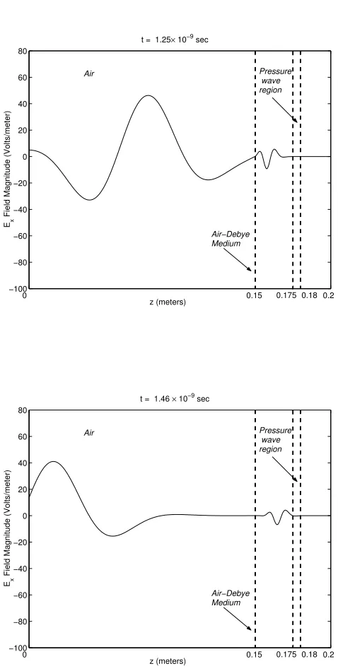
Figure 10: Forward simulation for a Debye medium with parameters given in (69) and (70). Plot of the magnitude of the Ex component of the electric field against z (meters). The input source is propagating towards the Debye medium.
0 0.15 0.2
−100 −80 −60 −40 −20 0 20 40 60 80
z (meters)
Ex
Field Magnitude (Volts/meter)
t = 1.04 × 10⁻⁹ sec
Air
Air−Debye Medium
Pressure wave region
0.175 0.18
0 0.15 0.2 −100
−80 −60 −40 −20 0 20 40 60 80
z (meters)
Ex
Field Magnitude (Volts/meter)
t = 1.25× 10⁻⁹ sec
Air
Air−Debye Medium
Pressure wave region
0.175 0.18
0 0.15 0.2
−100 −80 −60 −40 −20 0 20 40 60 80
z (meters)
Ex
Field Magnitude (Volts/meter)
t = 1.46 × 10⁻⁹ sec
Air
Air−Debye Medium
Pressure wave region
0.175 0.18
0 0.15 0.2 −100
−80 −60 −40 −20 0 20 40 60 80
z (meters)
Ex
Field Magnitude (Volts/meter)
t = 2.08 × 10⁻⁹ sec
Air
Air−Debye Medium
Pressure wave region
0.175 0.18
Figure 13: Forward simulation for a Debye medium with parameters given in (69) and (70). Plot of the magnitude of the Ex component of the electric field against z (meters). The interaction of the electromagnetic wave with the pressure wave causes the electromagnetic wave to partially reflect and partially transmit.
4.1
Sensitivity analysis
Here we examine the system dynamics as the parameters vary. We are interested in the changes produced by the coefficents of pressure in the polarization, namely the parametersκs,κ∞ andκτ. In Figure 15 we plot theEx component of the electric field for the simulation with parameter values given in (69) and four other simulations for which all the parameters, exceptκs, are fixed at the values given in (69). We change the value of κs to 0, 0.3s,0, 0.6s,0 and 0.9s,0, repectively, and plot the electric field
values for each of the corresponding forward simulations. As expected, by changing the value ofκs, we notice a change in the magnitude of the acoustic reflection observed at the center of the antenna.
In order to determine if the forward problem is sensitive to changes in the value of the pressure coefficient κ∞, in Figure 16 we plot the absolute value of the differences
in the Ex field component between simulations in which all the parameters except κ∞ are fixed at the values given in (69). The solid line in this figure represents
the difference in the Ex field magnitude between the forward simulation in which κ∞ = 0.8∞,0 and the simulation in which κ∞ = 0. The dashed line represents the
difference in the Ex field magnitude between the simulation in which κ∞ = 0.8∞,0
and the simulation in whichκ∞ = 0.2∞,0. We now determine if the forward problem
0 0.15 0.2 −100
−80 −60 −40 −20 0 20 40 60 80
z (meters)
Ex
Field Magnitude (Volts/meter)
t = 2.5× 10⁻⁹ sec
Air
Air−Debye Medium
Pressure wave region
0.175 0.18
Figure 14: Forward simulation for a Debye medium with parameters given in (69) and (70). Plot of the magnitude of the Ex component of the electric field against z (meters). The reflection from the acoustic pressure wave impinges on the air-Debye interface, while the wave transmitted into the pressure region moves into the right absorbing layer.
2 2.5 3 3.5 4
x 10−9 −1
−0.5 0 0.5 1
Time t (secs)
Ex
Field Magnitude (Volts/meter)
κs = 0
κs = 0.3εs,0 κs = 0.6εs,0 κs = 0.9εs,0
0 0.5 1 1.5 2 2.5 3 3.5 4 x 10⁻⁹
0 1 2 3 4 5 6 7x 10
−3
Time t (secs)
Absolute value of Difference in E
x
Field Magnitude (Volts/meter)
κ∞ = 0.8ε∞,0 , κ∞ = 0
κ∞ = 0.8ε∞,0 , κ∞ = 0.4ε∞,0
Figure 16: Plot of the absolute value of the difference in magnitude of theEx compo-nent of the electric field, between simulations in which κ∞= 0.8∞,0 and simulations
with different values ofκ∞, againstz (meters). The other parameters are fixed at the
values given in (69) and (70).
0 0.5 1 1.5 2 2.5 3 3.5 4
x 10−9
0 0.005 0.01 0.015 0.02 0.025
Time t (secs)
Absolute Value of Difference in E
x
Field Magnitude (Volts/meter)
κτ = 0.05τ0 , κτ = 0
κτ = 0.05τ0 , κτ = 0.2τ0
Figure 17: Plot of the absolute value of the difference in magnitude of theEx compo-nent of the electric field, between simulations in which the value of κτ = 0.05τ0 and
which all the parameters exceptκτ are fixed at the values given in (69). The solid line in this figure represents the difference in the Ex field magnitude between the forward simulation in whichκτ = 0.05τ0 and the simulation in whichκτ = 0. The dashed line represents the difference in the Ex field magnitude between the simulation in which κτ = 0.05τ0 and the simulation in whichκτ = 0.2τ0 From these plots we observe that
the parameterκsseems to be the most influential in the wave interaction, whereas the pressure coefficientsκ∞and κτ do not seem to be as influential. This observation can be supported from an analysis of (40). In our simulations the outgoing and reflected radiation will be dominated by frequencies near the center frequency 3.0 GHz. Thus, ∗
r will be dominated by frequencies near 3.0 GHz. In this problem ωτ0∗ ≈ O(10−2),
and 0 = 8×10⁻¹². Rewriting (40) as
∗
r = s 1 + jωτ +
jωτ 1 + jωτ
∞+
σ jω0
, (74)
we consider each of the three terms in (74) separately to determine their magnitude. The magnitudes of the corresponding true values of these three terms (neglecting the acoustic pressure terms) are approximately given as
∗
s,0
1 + jωτ∗ 0
≈ O(∗
s,0) ≈ O(10),
jωτ∗ 0
1 + jωτ∗ 0
∞,0 ≈ O(10−2∞∗ ,0) ≈ O(10−2),
σ∗
jω0
≈ O(102σ∗)
≈ O(10−3).
(75)
Thus we see that ∗
r will be most sensitive to the static permittivity s,0 and the
effects of ∞,0 and τ0 will not be as pronounced. Also, this implies that ∗r will be more sensitive to the pressure coefficientκsthan to the coefficientsκ∞ and κτ, which
coincides with the observation that was made from Figures 15, 16 and 17
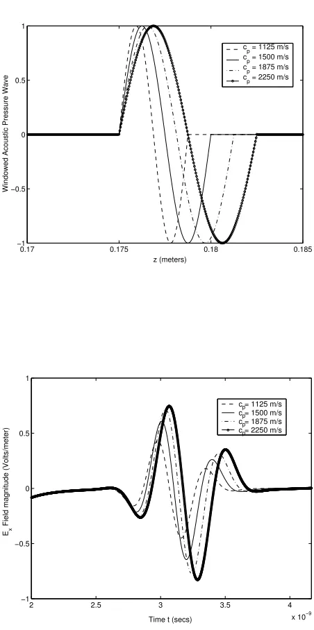
We would also like to see what effect the acoustic speed and frequency have on the amplitude of the reflection from the acoustic pressure region. In Figure 18 we plot the acoustic reflection observed at the center of the antenna for different values of the acoustic frequency and in Figure 19 we plot the acoustic reflection for different values of the acoustic speed. By changing the speed or the frequency, the wavelength λp changes and thus the size of the interval (z2, z2+λp) in which the pressure wave is
0.17 0.175 0.18 0.185 −1
−0.5 0 0.5 1
z (meters)
Windowed Acoustic Pressure Wave
fp = 2.0 × 10⁵ Hz
fp = 3.0 × 10⁵ Hz
fp = 4.0 × 10⁵ Hz
fp = 6.0 × 10⁵ Hz
2 2.5 3 3.5 4
x 10−9 −1
−0.5 0 0.5 1
Time t (secs)
Ex
Field Magnitude (Volts/meter)
fp = 2.0 × 10⁵ Hz fp = 3.0 × 10⁵ Hz fp = 4.0 × 10⁵ Hz fp = 6.0 × 10
5 Hz
0.17 0.175 0.18 0.185 −1
−0.5 0 0.5 1
z (meters)
Windowed Acoustic Pressure Wave
cp = 1125 m/s cp = 1500 m/s cp = 1875 m/s cp = 2250 m/s
2 2.5 3 3.5 4
x 10−9 −1
−0.5 0 0.5 1
Time t (secs)
Ex
Field magnitude (Volts/meter)
c = 1125 m/s c = 1500 m/s c = 1875 m/s c = 2250 m/s
p p p p
5
Parameter estimation and statistical inference:
The inverse problem
In our forward simulations the signal that we record at the center of the antenna is a set of measurements of Ex, the x component of the electric field, at the point (0, zc) in our computational domain at discrete, uniformly spaced intervals of time. This signal has components consisting of the input source, the reflection at the air-Debye interface and another reflection from the region that contains the pressure wave as seen in Section 4. The signal is a function of the various dielectric properties of the Debye medium; namely, the static relative permittivity s,0, the infinite frequency
permittivity ∞,0, the relaxation time τ0, the conductivity σ, and the three pressure
coefficients κs, κ∞ and κτ. We collect all these quantities together to define the parameter vector
q= [s,0, ∞,0, τ0, σ, κs, κ∞, κτ]T. (76)
Thus, the signal recorded in the forward simulation is a function of q, and changing the value of q will change the signal that is recorded. In general, such signals are usually obtained in an experimental setting conducted in a laboratory with physical equipment such as electric pulse generators to generate electric pulses, piezoelectric transducers that generate the acoustic pressure waves and antennas/receivers that record the electric field intensities. Moreover, such signals generated in an experi-mental setting are usually noisy, with noise arising through the equipment that is used; namely the resistor, antenna/receiver and the transducer, in our case. Implicit in such collection of measurements is the assumption that there exist true values of all the parameters that characterize the medium to be interrogated. We will denote the corresponding true parameter vector byq∗.
In order to simulate an experimental situation (i.e., generate typical “data”) we assume that there exist true values of all the parameters involved in our problem, and we use these true values (which of course would not be known in an experimental setting!) in our forward simulation, viz. the FDTD method and record the signal observed at the antenna as described above. We then add noise to the generated signal to produce a noisy signal which will form theobservationsordatathat we will use in an inverse problem, as a substitute for data generated in the laboratory. The goal of our electromagnetic interrogation technique is to identify or estimate the true parameter q∗ that characterizes the particular Debye medium being interrogated, from data
that consists of a signal recorded at the center of the antenna. The reason for using simulated data in the inverse problem is to validate the methods first on “data” from known parameters in a setting with known noise. If we cannot estimate the dielectric parameters from data that is constructed via numerical simulations of our discrete model, then the reconstruction of these parameters from actual experimental data usually will not be feasible.
solve as follows: Using observations or data (electric field intensities containing noise collected at the center of the antenna), determine an estimateˆq, of the true parameter q∗, that belongs to an admissible set Q, so that the solution of the forward problem with q = ˆq best describes the data that is collected. When we have solved this deterministic problem (as will be detailed below), it will also be necessary to specify reliablility of our estimates, i.e., can we specify measures of uncertainty related to the estimate ˆqof q∗? It is important to note that the uncertainty in consideration is
inherent in the method of producing the estimates as well as in the process of data collection. Such measures of uncertainty will be specified by means of confidence intervals. These intervals are a probability statement about the procedure which is used to construct estimates of the parameters. Thus we are led in a completely natural way to stochastic or probabilistic aspects of estimates from a deterministic problem solved with deterministic algorithms [BB99]. The statistical error analysis that we will present here is based on standard statistical formulations as given in [DG95].
We first consider the two different ways in which we can add noise to our signal, i.e., the values of the x component, Ex, of the electric field observed at the center of the antenna, (0, zc), for different times tk =k∆t, k = 0,1, . . . , M. We represent this signal as the vector
(i) E(q∗) ={E∗
k}Mk=1 = (Ex(t1,0, zc;q∗), . . . , Ex(tM,0, zc;q∗))T ,
(ii) q∗ = (∗
s,0, ∗ ∞,0, τ
∗
0, σ
∗
, κ∗
s, κ
∗
∞, κ
∗
τ)T,
(77)
q∗ being the true parameter vector.
1. Relative random noise (RN) : In this case the amplitude of the noise that is added is proportional to the size of the signal, {E∗
k}Mk=1. Our simulated data is
Oks =E∗
k(1 +νηks), k= 1, . . . M, (78)
where ¯η={ηk}Mk=1 are independent normally distributed random variables with
mean zero and variance one, i.e., ηk ∼ N(0,1), k = 1, . . . , M. We express the relative magnitude of the noise as a percentage of the magnitude of E(q∗) by
taking two times the value ofν as the size of the random variable. For example, ν = 0.005 corresponds to 1% relative noise [BBL00]. This noise model does not produce constant variance across the samples.
where as in (78), ηk ∼ N(0,1), k = 1, . . . , M. The constant β is taken to be the product να, where α is a scaling factor which is chosen so that the signal to noise ratio (SNR) of the data defined in (79) corresponds to data defined in (78) with noise level ν. This justifies comparing results obtained with the two different ways of adding comparable noise to our signal. This will be addressed in more detail in Section 5.
The vectorOs ={Os
k}Mk=1 will be our data or observations, and the noise ¯η={ηk}Mk=1
will be referred to as the measurement errors corresponding to the observations. The statistical error analysis that we now develop is only applicable to the case of constant variance noise. Thus, for the rest of this section, we will assume that our observations are of the form (79). The sample observations Os, which are in general obtained from experiment, are a realization of the corresponding random variable O = (O1, O2, . . . , OM)T which can be seen to be a transformation of the random variable ¯η. Thus
Ok =Ek∗+βηk, k = 1, . . . M, (80)
is a stochastic process and has a multivariate normal distribution with mean vector E(q∗
) defined in (77, i) and covariance matrix β2I
M. The statistical model
O∼NM{E(q∗), β2I
M}, (81)
is a formal representation of thepopulationof all possible realizations ofO1, O2, . . . , OM that can be observed. When we collect data, we are observing a single realization of Os
1, . . . , OsM i.e., a sample. Our objective then is to estimate the true value of the parameter q∗ by collecting data, i.e., observing a single realization of O as well as
accounting for the fact that a different realization will produce a different estimate of q∗. We would like to learn about the true value q∗ (which determines the nature of
the population) from a sample, as well as indicate the certainty (or uncertainty) that we can associate to our knowledge of this parameter. This process of making state-ments about a population of interest on the basis of a sample from the population is called statistical inference.
The unknown true parameters vector q∗ will be estimated by means of a
suit-able function ˆq(O) of the observations O. The function ˆq(O) is a random vari-able and is referred to as an estimator. When evaluated at a particular realization, Os
1, Os2, . . . , OsM, this estimator yields a numerical value that gives information about the true value of the parameter q∗. For a particular realization Os of the random variable of observations O, we callqˆ(Os) anestimate. In this report we will consider the method of least squares to obtain estimates for the parameters and to calculate confidence intervals for the estimates by linearizing around the estimate qˆ(Os). In this case ˆq(O) will be the least squares estimator ˆqOLS(O). Associated with the ran-dom variableˆqOLS(O) is the probability space Q= (Q,B, m), where Q is the sample