ABSTRACT
JETLY, GAURAV.A Multi-Agent Simulation of the Pharmaceutical Supply Chain. (Under the direction of Russell E. King.)
A Multi-Agent Simulation of the Pharmaceutical Supply Chain
by Gaurav Jetly
A thesis submitted to the Graduate Faculty of North Carolina State University
in partial fulfillment of the requirements for the degree of
Master of Science
Industrial Engineering
Raleigh, North Carolina 2010
APPROVED BY:
______________________ ______________________
Dr. Russell E. King Dr. Christian Rossetti Chair of Advisory Committee Co-Chair of Advisory Committee
______________________ ______________________
BIOGRAPHY
ACKNOWLEDGEMENTS
I owe my deepest gratitude to Dr. Christian Rossetti, co-chair of my committee, who gave me this opportunity to learn and do research under his guidance. I am also thankful to him for his patience and excellent guidance throughout my research work and for sharing his vast knowledge with me. Dr. Rossetti has always been very helpful, motivating, and encouraging which enabled me to enhance my understanding of the subject.
I am also grateful to Dr. Robert Handfield who involved me in his research group and also supported and encouraged me at every stage of the project. His words of encouragement kept me in high spirits through out my research work.
I am also thankful to Dr. Kay and Dr. King. Dr. Kay has helped me in becoming a better programmer. I felt a great difference in my programming abilities after completing my course in Logistics Engineering. Dr. King helped me identify my career goals and also guided me in achieving those goals. I am also thankful to Dr. King and Dr. Kay for a thorough review of my thesis.
I would also like to thank all the faculty members at North Carolina State University who taught me different courses.
TABLE OF CONTENTS
LIST OF TABLES ... vi
LIST OF FIGURES ... vii
Chapter 1 Introduction ... 1
1.1 Background ... 1
1.2 Research Questions ... 3
1.3 Layout of the Dissertation ... 3
Chapter 2 Literature Review... 4
2.1 Pharmaceutical Industry ... 4
2.2 Multi Agent Simulation ... 6
Chapter 3 Methodology ... 9
3.1 Identify the Supply Chain Structure and Interactions ... 9
3.2 Data Mining and Analysis ...11
3.3 Develop Algorithm and Rules for the Agents ...14
3.4 Develop the Model using the Java Programming Language ...21
3.4.1 Supplier Object ...21
3.4.2 Manufacturer Object ...24
3.4.3 Distributor Object ...28
3.4.4 Global Attributes ...31
3.4.5 Statistics Methods ...32
3.4.6 Data Collection and Other Features ...32
Chapter 4 Results ...41
Chapter 5 Summary and future work ...45
REFERENCES ...48
APPENDIX ...51
LIST OF TABLES
Table 1: Different stages of drug development ...12
Table 2: Rules for individual players and for their interaction ...19
Table 3: Supplier Object Properties ...22
Table 4: Manufacturer Object Properties ...25
Table 5: Distributor Object Properties ...29
Table 6: Global Variables Properties ...31
Table 7: Number of simulations conforming to industry data at 5 percent significance level ... ..35
Table 8: Analysis of Variance ...41
LIST OF FIGURES
Figure 1: Interaction in pharmaceutical supply chain ...10
Figure 2: Mergers at each level of pharmaceutical supply chain ...11
Figure 3: Cost of drug development ...13
Figure 4: The product life cycle curve for different types of drugs ...14
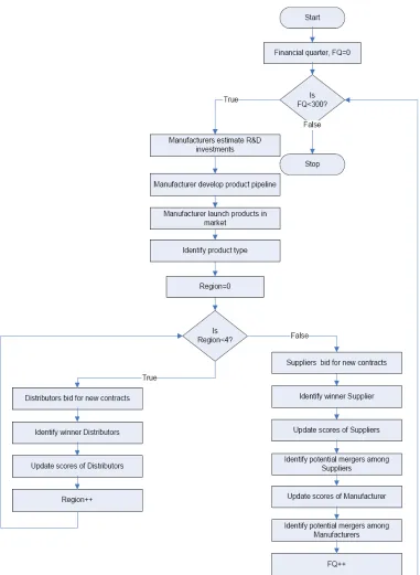
Figure 5: Simplified schematic of simulation flow in the model ...16
Figure 6: Different classes and their interaction ...33
Figure 7a: Simulation output for the games with KS test statistic< critical value ...36
Figure 7b: Compustat data for the large pharma companies of 1982 ...36
Figure 8a: Simulation output for the games with with KS test statistic< critical value ...38
Figure 8b: Orange book data for the large pharma companies of 1982 ...38
Figure 9a: Simulation output for the games with KS test statistic< critical value ...39
Chapter1
Introduction
1.1 Background
The movement of pharmaceutical product from manufacturers to its consumer involves several players. These are suppliers, manufacturers, distributors, pharmaceutical benefit managers, health insurance companies, and pharmacies/retailers. Competition and uncertainty at each of these levels has made the pharmaceutical supply chain one of the most dynamic sectors of United States economy. Besides being the biggest market of pharmaceutical drugs, the United States is also a pioneer in terms of discovery and development of new drugs. Out of the top 20 largest pharmaceutical companies, 12 are based in the USA. A large contributor to the dynamics of the pharmaceutical industry is new product development. The spending on research and development (R&D) relative to sales revenue is highest in the pharmaceutical industry –spending increased from $5.5 Billion in 1980 to more than $17 Billion in 2003 as per CBO report. Despite large increases in drug R&D spending over the last 25 years, there is little increase in the number of new drugs entering the market each year.
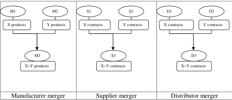
Further, there are drug specific contracts between suppliers, manufacturers and distributors that give rise to complex, competitive and dynamic relationships in the pharmaceutical supply chain. The industry is also marked with large number of mergers and acquisitions (M&A) over last 30 years. At the manufacturer level M&A were primarily a response to perceived lower than expected earnings. Distributors merged to expand their market and to reduce operational cost. At the distributor level the consolidation resulted in three large players (AmerisourceBergen, Cardinal, and Mckesson) sharing more than 90 percent of the drug distribution industry.
The dynamics and evolution of the pharmaceutical supply chain is governed by a number of forces and their interaction. In the literature these factors have been studied, but most of the studies focused on individual factors such as R&D, profitability, costs etc. and do not address the role of complex and dynamic relationships that exist between the members of the pharmaceutical supply chain. Also, the existing research on pharmaceutical industry does not consider the impact of competition and the supply chain structure on the profitability of industry.
1.2 Research Questions
The objective of this study is to develop a model which includes all the governing factors along with the complex, competitive and dynamic relationships that exist in the pharmaceutical supply chain. Due to the importance of the pharmaceutical industry and the dynamic interplay between manufacturing systems, product lifecycle, and government regulation, this research addresses following questions:
1. How should various forces and agents (Manufacturers, Suppliers, and Distributors) in the pharmaceutical supply chain be modeled?
2. Do certain structures result in superior supply chain financial performance?
1.3 Layout of the Thesis
In the next section of the thesis, some applications of multi-agent methodology in different domains are summarized. Chapter 3 is focused on the methodology adopted to develop the model. The methodology section is further divided into subsections explaining the different stages of model development.
Chapter 4 explains how the model was validated using industry specific data obtained from Compustat, Congressional Budget Office, and the FDA and industry reports. Various non-parametric and parametric techniques were used to validate the model.
Chapter2
Literature Review
2.1 Pharmaceutical Industry
There have been a number of studies focused on different areas in pharmaceutical industry. Each of these studies looked at different aspects of the industry and followed different methodology. The empirical research addresses three intersecting areas: profitability, research intensity, and mergers and acquisitions.
The pharmaceutical industry is considered to be the most profitable industry as measured by returns on investment in R&D. Several studies have investigated returns to R&D expenditure (Grabowski and Vernon, 2003). Most of the studies concluded that the returns were much higher than other industries due to extensive research and innovation. Other studies focused on the efficiency of new product development and if there is a relationship between firm size and research productivity (Henderson and Cockburn, 1996). DiMasi, Hansen and Grabowski (2003) have extensively examined time and cost of new drug development. They derived the costs in different stages of drug development using the phase transition probabilities for an investigational new drug. The authors estimated that out of pocket cost was $403 million per approved drug and total cost of capital was $ 802 million per approved drug.
to 15 percent since 1980. The reason for an increase in R&D investment is an increase in sales revenue from pharmaceutical products. The drug development process involves various stages and overall has a very low success rate. A large number of new molecular entities need to be tested by manufacturers to discover the molecular entities with a potential to clear the clinical trials. On an average, 5 out of every 5000 compounds tested clear the preclinical stage. Due to low success rate, large scale research efforts are required to discover a new drug.
Extrapolating from the previously mentioned empirical results is questionable due to sample size and multiple exogenous shocks. In addition, empirical research on supply chain relationships is lacking. The nature and effects relationships between manufacturers, suppliers, and distributors are relatively untouched by management researchers. This is understandable given the difficulty in collecting detailed data on contracts, R&D, and M&A from three members of a supply chain.
2.2 Multi-Agent Simulation (MAS)
allocate limited resources of an enterprise across the available product investment opportunities to achieve the best possible returns. Therefore their study was a firm specific study and does not include other players in the industry like suppliers, distributors and other manufacturers.
therefore does not help us understand the impact of this dynamic force on the supply chain relationship.
Chapter 3
Methodology
In the early phase of this study, a conceptual model (Balci and Ormsby, 2007) was developed based on different industry reports and research findings. The conceptual model was used during simulation design and implementation stages. The Simulation model was developed in the following stages:
1. Identify the supply chain structure and interactions, 2. Perform data mining and analysis,
3. Develop algorithm and rules for the agents,
4. Develop the model using the Java programming language, 5. Perform model verification and validation
3.1
Identify the Supply Chain Structure and Interactions
The pharmaceutical supply chain involves multiple players with different roles. In our model, we considered three levels of the supply chain: suppliers, manufacturers, and distributors. These players, at different levels of supply chain, have different roles and therefore are modeled as different types of agent. There are two general types of interaction in pharmaceutical supply chain (refer to Figure 1): vertical interaction and horizontal interaction. Vertical interaction involves product specific contracts and bidding.
Figure 1. Interaction in pharmaceutical supply chain (arrows represents bids for the new product).
Manufacturer merger Supplier merger Distributor merger Figure 2. Mergers at each level of pharmaceutical supply chain.
3.2
Data Mining and Analysis
The data were extracted from several databases such as the COMPUSTAT database (2008), the FDA’s Orange book (2008), several technical papers and reports. Different simulation parameters and rules were estimated using this data. Random scores, representing the firms’ assets, are assigned to each type of player at the start of the simulation. Scores are based on a triangular distribution, TRIA (minimum, mode, maximum) that has been fitted to the log of the firms’ total assets in their specific standard industrial code (SIC). The parameters are based on 1982 data from the COMPUSTAT database (2008). For manufacturers the parameters are: TRIA(4.20,7.63,9.00). For suppliers the parameters are TRIA(3.72, 7.15, 8.52). For distributors the parameters are: TRIA(2.00 , 3.10, 7.76). Each time a simulation starts, new starting scores for each type of agent are obtained from these distributions.
M1 M2
M3
X products Y products
X+Y products
S1 S2
S3
X contracts Y contracts
X+Y contracts
D1 D2
D3
X contracts Y contracts
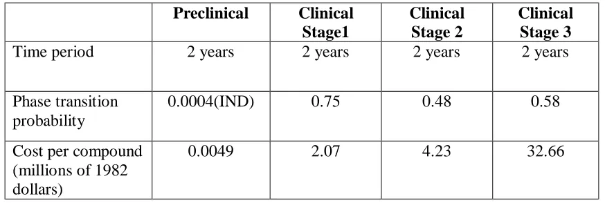
Each manufacturer has its own product pipeline under development. In our model, we used the drug development estimates from the findings of DiMasi et al. (2003). In their study, the product development was categorized into two stages: preclinical and clinical. The average drug development period is eight years. The preclinical stage varies for different drugs from 1-6 years. The clinical stage is subcategorized into stage1, stage2, and stage 3. In our model, preclinical stage and each subcategory of clinical stage is spread across 2 years. Based on DiMasi et al. (2003), estimates of drug development cost in each stage of preclinical and clinical trials and using the probabilities of success in each stage, we determined the cost of preclinical and clinical trials as well as the probability that each investigational new drug (IND) would advance to the next stage. The timeframes for each stage and the probabilities of success at the end of each stage are presented in Table 1 (DiMasi, Hansen, and Grabowski, 2003).
Table 1. Different stages of drug development (time and the probability of success)
Preclinical Clinical
Stage1
Clinical Stage 2
Clinical Stage 3
Time period 2 years 2 years 2 years 2 years
Phase transition probability
0.0004(IND) 0.75 0.48 0.58
Cost per compound (millions of 1982 dollars)
0.0049 2.07 4.23 32.66
*http://www.fdareview.org/approval_process.shtml
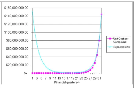
successful product, a cost per compound was estimated in different stages of product development (refer to Figure 3).
Figure 3. Cost of drug development (where average drug development time is 8 years)
Figure 4. The product life cycle curve for different types of drugs.
Based on an industry report published by Pharmaceutical Research and Manufacturers of America (2006), we considered effective patent life to be 12 years. Further, each drug follows a different sales trajectory with sales concentrated mostly before the patent expiration. The model also includes the drug price increases due to inflation. The Congressional Budget Office (2006) estimates that drug prices have increased at three times the increase in the consumer price index (CPI). Therefore, although base revenue (demand) is driven by the lognormal curve, revenue each quarter is inflated by the Drug Price Index (DPI). We assume that all input costs will rise with inflation and affect each player similarly.
3.3 Develop Algorithm and Rules for the Agents
financial quarter. We ran the simulation for 300 quarters, which is equivalent to 39 years. At the beginning of the simulation game, scores/assets are assigned to each kind of player based on their corresponding triangular distribution. The initial 144 quarters are taken as a warm up period during which scores of different players do not change. The warm up period of 144 quarters represents three complete product life cycles.
During the simulation warm-up period a product pipeline is developed for each manufacturer. Manufacturers spend on R&D based on the square root of their assets. The square root of assets is used to represent the findings that smaller pharma firms tend to have a more focused product pipeline with fewer resources to support its R&D. Large manufacturers tend to have a larger and more diversified product pipeline. During the warm up period, the manufacturers’ assets remain constant. That is, products released do not create profits and the pipeline is costless.
based on the conditional probabilities of success in that stage. The actual industry R&D/Sales ratio ranged from 0.15 to 0.21 (Congressional budget office (2006) report mentions the finding of two studies. The first one was based on a report from the Pharmaceutical Research and Manufacturers of America (2005). They found that R&D/Sales ratio varies between 15 to 19 percent. They also mentioned the findings of National Science Foundation study in which it remains close to 15 percent) during the period under consideration (Congressional Budget Office, 2006). In our simulation, manufacturers spend 15 % of their overall sales on R&D in each financial quarter.
When a product is launched in different markets, it follows one of the three product life cycle curves. The sales for these drugs follow a lognormal distribution with different parameters for small, medium and blockbuster drugs based on the findings of Grabowski and Vernon (1993, 2003). These drugs are released by the manufacturers based on the rules described in Table 2.
In our model, we divided the pharmaceutical market into four regions with sales proportional to population in each region. We populated each region with a different number of distributors proportional to the population in that region.
quarter the distributors update the average returns from the existing products for each manufacturer. For a new product, their estimated bid value is equal to this updated average from each manufacturer. For an exisitng product, distributors estimate the demand in next two years based on historical demand for that product. Based on the bid values received, the manufacturer determines the winning distributor.
Suppliers estimate their bid value based on their performance in the previous two bidding rounds. If they lost the previous two bids, they reduce their next bid value by a small percentage (determined using a random number generator). In cases where they win any of the previous two bids, they increase their next bid value by a small percentage. Every quarter, suppliers update the number of active contracts with each manufacturer. Active contracts with a manufacturer are the number of contracts a supplier won with that manufacturer in the last 12 years. In case the bid value of two suppliers is equal, the manufacturer selects the supplier with greater number of active contracts. This is similar to industry practices where previous relationships hold sway in supplier selection decisions.
Every quarter, different players receive returns from the active products and bear different costs based on the rules described in Table 2. Their profit from each product depends on the product life cycle (Figure 4) and the product type (Table 2).
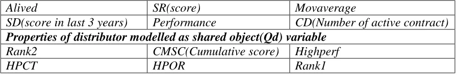
Table 2: Rules for individual players and for their interaction
Manufacturer Supplier Distributor
Starting bid Number of Agents Bid based on
Costs
Profit Margin
Bid Estimation rule
M & A rule
Other
N/A 30 N/A
10% of sales(marketing cost), 15% of sales on R&D Suppliers Margin 33% tax on net earnings
80%, 85%, 90% for small, medium and large products.
N/A
Manufacturers merge if: 1.Score1 > 5 X Score2. 2.Ln(HPOR2**)>1
3.HPOR is calculated based on return to assets and their product pipeline in last stages of development. After each round, Odds ratio (HPOR) is updated. 4.Determine the priority given to players for bidding based on multi criteria rank order based on their performance and Assets 5.Merger does not reduce
Herfindahl index to less than 0.2
Drugs are released by Manufacturers if the IND under clinical trial clears all stages.
The type of drug is decided based on the random number(RN)
• RN<=3 => small drug
• 3< RN <9 => medium drug
• RN >=9 => Block buster. .
10 60
Acceptable profit margin 5% of Assets
Based on bid value If lost previous 2 rounds Bid= Last round bid – RN*
(0-0.1).
If won at least 1 of the previous 2 rounds
Bid= Last round bid+RN*(0-0.1). Suppliers(1 & 2) merge if: 1.Assets1 >1.5 X Assets2 2.Ln(HPOR2**)>1
3.HPOR is calculated based on return to assets. After each round, Odds ratio (HPOR) is updated.
4.Determine the priority given to players for bidding based on multi criteria rank order based on their performance and Assets
5.Merger does not reduce Herfindahl index to less than 0.2
10
60(15,24,12,9 in each region) Future market share, historical demand, previous products 3% of Assets
10%
If Expected bid > 10 % of Assets then bid= 10% of the Assets. If Expected bid < 10 % of Assets then bid= Returns.
Distributors(1 & 2) merge if:
1. Assets1 >5 X Assets2
2. Mergers occur only within a region.
3. Ln(HPOR2**)>1
4. HPOR is calculated based on return to assets. After each round, Odds ratio (HPOR) is updated.
5. Determine the priority given to players for bidding based on multi criteria rank order based on their performance and Assets
6. Merger does not reduce Herfindahl index to less than 0.2
Demand is distributed in the 4 regions in the following ratio: 0.25, 0.40, 0.19, 0.16 Distributor gets the distribution rights for the drug till the contract time frame. Once the contract is over, all the distributors in that region bid again.
*Random Number
**HPOR refers to High Performance Odds Ratio. It is estimated using different performance indicators for different players. For suppliers, and distributors, the performance indicator is based upon profitability in recent years. For manufacturers, the performance indicators are based upon products in R&D pipeline and profitability in recent years. These performance indicators are estimated as follows:
Performance1: (Profit in last 3 years)/(Current score)
Performance2= (Number of drugs in stage2 and stage3)/(Current score)
Table 2 Continued
which is a measure of number of quarters in which a firm performance was above median. Next we estimate Odds ratio from the HPCT as follows:
High performance odds ratio (HPOR) = ((HPCT1+ HPCT2)/(24-HPCT1-HPCT2))2
If, ln( HPOR) >1 then the company is a suitable target firm. This condition ensures that the company under consideration either has above average product development pipeline or has above average number of products in market which are in early stage of the life cycle. Among the acquiring companies the priority to bid goes to the manufacturer with a higher rank based on weighted average of their Assets and returns on assets (ROA) in last 3 years. Acquirer should have high capital reserve which is required to support the R&D, marketing and manufacturing of products of both the companies. The weight assigned to ROA is less than the weight assigned to Assets. This ensures that the acquiring company has good capital reserves. Another restriction is on the industry concentration. Any acquisition should not result in the industry herfindahl index to cross 0.2 which is considered as a very high concentration level in any industry. For suppliers and distributors, only one performance indicator was considered to measure HPCT and HPOR.
assets, with weights assigned to each criterion to calculate the ranking. This multi-criterion approach is reflected in practice where the largest and most profitable companies have easiest access to capital, which can then be used for acquisitions. Similarly, the most attractive manufacturer to be acquired is determined by the number of products in stage 2 and stage 3 of the product pipeline and their profitability during the last three years. After a merger, the products and contracts of the merging manufacturers are assigned to the new manufacturer. For distributors mergers are based on relative profitability in the previous three years as described in Table 2. The priority bidder will be the one with highest weighted score based on assets and performance in last three years. The new distributor has the combined experience of the type of products launched by the different manufacturers from the history of both distributors. This gives it an advantage in future bidding. Similarly, each supplier determines the ideal candidate for merger according to the rules described in Table 2 and merge. The new supplier has active contracts of both the suppliers.
supply chain network, associated suppliers and distributors of the two manufacturers are assigned to the new manufacturer.
3.4 Develop the Model using the Java Programming Language
The pharmaceutical supply chain multi-agent simulation was developed in JAVA. The simulation was developed in small modules and sub modules following it. Initially two levels of supply chain were developed and later third layer was added. We divided the simulation into a Main class (which forms the flow of the simulation as mentioned in the Figure 5) and other classes each representing different types of agents. There is a separate class for suppliers, distributors, and manufacturers, each with their own specific attributes and methods. Further each agent has its own thread of control. A new thread is generated whenever merger happens and the threads corresponding to old agents become inactive.
3.4.1 Supplier Object
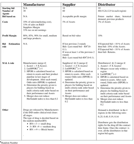
The Suppliers object has several properties and routines to interact with other objects in the simulation and to perform several tasks autonomously like bidding, determining potential candidates for mergers, and estimating their profits from their active contracts. 3.4.1.1 Supplier Object Properties
manufacturers. Properties like Performance keep track of their Return on Assets over the last 3 years. Rank1 and Rank2 determine the relative ranking of suppliers based on their
Performance and Score respectively. Further their relative Rank is estimated based on the cumulative score CMSC obtained by taking weighted average of Rank1 and Rank2. The higher Rank suppliers get priority over other suppliers during the acquisition process. Further potential candidates to be acquired are determined based on HPOR (High performance odds ratio) over the last 3 years. HPOR is determined based on Highperf and HPCT (High performance count). Table 3 summarizes all the Properties associated with Supplier Object.
Table 3: Supplier Object Properties
Alives Score(s) CA( Number of active contracts)
Averageprofit Performance Sa(Score over the last 12 rounds)
Supplier Number
Properties of supplier modeled as shared object(Qs) variables
Rank2 Rank CMSC(Cumulative score)
Highperf HPCT(highperformance count) HPOR(high performance odds ratio)
Rank1
3.4.1.2 Supplier Object Methods
Suppliers take decisions and perform their actions using a number of methods. These methods implement the rules mentioned in Table 2. Suppliers use these methods to determine the bids, profits, performance and to update their scores. These methods are discussed below. Bid
two bids, it increases its previous bid by a small value estimated using random number generator.
Bidnew
In case the supplier lost both the previous bids, it decreases its bid by a small value determined using random number generator. This is done by the supplier to ensure that it has sufficient business for sustaining in the industry.
Profits
This subroutine is used by the supplier to determine the profits they make from each product for which they won the contract in the last 12 years (Effective patent life). Their bid value represents their profit margin. Based upon this bid value they receive profit every quarter.
Contractwon
Supplier agents use this subroutine to estimates the number of contracts which were won by the supplier, and the number of active contracts with different manufacturers.
Scoreupdate
Supplier loses the operational cost and updates the profits from active contracts with different manufacturers. Once the score is updated, it is written in the text file.
Inflation
This method is used to estimate the inflation factor in any particular round. Relativeperformance
This method is used to carry out following three tasks:
2. Update the property called performance = (Current score- score 3 years back)/current score
3. Update the score in last 12 rounds and performance value into the shared object called
Qs
Sums
Estimate and returns the sum of an array which was passed to this method. This subroutine is used by a number of other subroutine during their execution.
3.4.2 Manufacturer Object
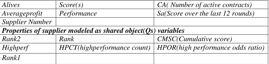
The Manufacturer object also has properties and methods similar to the suppliers which it uses to interact with other players (Table 4).
3.4.2.1 Manufacturer Object Properties
Manufacturers interact with both suppliers as well as distributors in different regions. Also they have other properties like product pipeline and products in market. Therefore, they have much greater number of object attributes as compared to suppliers. Properties associated with Mergers, Scores and Performance is similar to that of supplier. Manufacturer objects have other object properties like Products (Index number to identify product) and TR
shared objects and these shared objects are used to store the values of some of the above attributes like Products(P), Wind(Winner distributor), Wins(Winner supplier), Winbidd( winning bid value of distributors), Winbids(winning bid value of supplier) etc.
Table 4: Manufacturer Object Properties
Alivem Performance Performancep
NME(Number of New
molecular entities in
product development
pipeline)
SM(Score of Manufacturer) SM1(Score of Manufacturer over last 3 years)
Properties of manufacturer modelled as shared object(Glob) variable
Products(P) Tr(Year of launch of product) B1(Product category)
Winbids(Bid value of
winner supplier)
Winbidd(Bid value of winner distributor)
Wind(Winner distributor)
Wins(Winner Supplier)
Properties of manufacturer modelled as shared object(Qm) variable
Highperf Highperfp Rankp
HPOR HPCT Rank1
Rank2 Rank
3.4.2.2 Manufacturer Object Methods
Manufacturers also take decisions and perform their actions based on a number of methods. They use these methods to determine their profits, performance and to update their scores and to determine their investment in R&D. They also use different methods to select a supplier/ distributor for their new products. These methods are discussed below.
Mini
Winner
This subroutine returns the index number of winner supplier or distributor whenever bidding event occurs. For suppliers, it returns the index number of supplier with the lowest bid value. For distributors, it returns the index number of distributor with the highest bid value.
Nextbidyear
Distributors win the contract for the product for a certain time frame based on their bid value. This subroutine determines the financial quarter in which the next bidding will occur after the end of existing contract. A supplier agent can win a contract for the entire product lifecycle whereas a distributor can win a contract for a maximum of two years. Profits
Manufacturers use this method to determine their revenue each quarter from the products which they have launched in last 12 years. Their revenue is based upon the type of products and the corresponding profit margin (as mentioned in Table 2).
PipelineCost
Manufacturers use this subroutine to determine the cost of Research and Development (R&D) of their existing pipeline. It calculates the cost of clinical trials for all the products in different stages of clinical/ preclinical testing.
Approval
Manufacturers determine if they can support the entire pipeline with their assets or not. If their assets are not sufficient to support the entire product pipeline, they spend their assets on part of their pipeline which is closest to the market. If the capital assigned for R&D is sufficient to support the entire pipeline, they spend the leftover capital on testing New Molecular Entities (NME’s). This function also determines the number of drugs which successfully clears each stage and moves over to the next stage. Therefore it also determines the successful drugs entering next stage of drug development for the entire product pipeline. Basepdapproval
During the simulation warm up period, manufacturers use this subroutine to determine the number of drugs which successfully clear different stages of drug development to reach the next stage.
Scoreupdate
Manufacturer updates its score in following steps: 1. Score = Score - R&D expenditure
2. Score = Score - 10% of profit in previous round
3. Score = Score - 33% corporate tax on the net profit in this financial quarter (Current score - score in previous round)
4. Score = Score + Profit from active products - Suppliers margin based on their bid value
5. Write the updated score in the text file Assignproductcategory
1. Update the year launched for the new products
2. Assign the category to the product based on random number generator:
• If Random number <= 3 then it is a small product
• If Random number > 3 and Random number < 9 then it is a medium product
• If Random number >= 9 then it is a blockbuster product 3. Estimate the next bid year for the new product launched
Relativeperformance
This method performs the following tasks:
1. Update the array which stores the score for last 12 rounds 2. Estimate performance based on score:
3. Performance = (Current score - score 3 years back)/current score
4. Performancep = (Number of products in R&D pipeline in stage 2 and stage3)/current score
5. Update the performance and score data in shared object called Qm Inflation
Estimate the inflation factor for the current round
3.4.3 Distributor Object
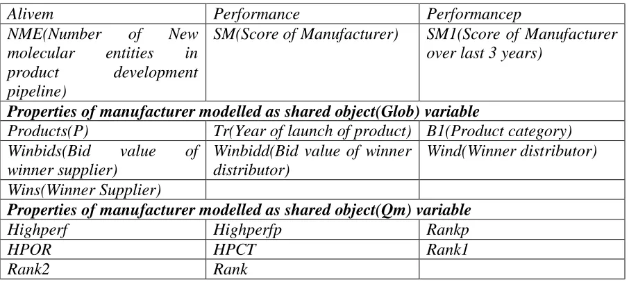
Distributor also has several attributes and methods to interact with manufacturers. 3.4.3.1 Distributor Object Properties
Table 5: Distributor Object Properties
Alived SR(score) Movaverage
SD(score in last 3 years) Performance CD(Number of active contract)
Properties of distributor modelled as shared object(Qd) variable
Rank2 CMSC(Cumulative score) Highperf
HPCT HPOR Rank1
3.4.3.2 Distributor Object Methods
Distributors also take decisions and perform their actions based on a number of methods. These methods implement the rules mentioned in Table 2. They use these methods to determine the bids, profits, performance and to update their scores. These methods are discussed below.
Bid
This method is similar to those of supplier except that in case of distributors if they loose the previous two bids they increase their bid value. This method is used by distributors only during the simulation warm up period.
Bidnew
This method is similar to those of supplier except that distributors use this method if they won atleast one of the previous two bids. This method is used by distributors only during the simulation warm up period.
Update
Profits
This method is used by the distributors to determine the profits from the products for which they won contract in last 12 years.
Contractwon
This method updates the number of contract won by the distributor and the number of active contract of distributor with each manufacturer.
Scoreupdate
1. Distributor loses the operational cost
2. It updates the profit from all the active contracts. Distributor receives 10% of the over all sales of a particular product in its region as its profit.
3. Write the updated score into text file. Inflation
This method is used to estimate the inflation factor in any particular round. Relativeperformance
This method is used to carry out following three tasks:
1. Update the array which stores the score of distributor in last 12 rounds
2. Update the property called performance = (Current score - score 3 years back)/current score
3. Update the score in last 12 rounds and performance value into the shared object called
Qd
Sums
3.4.3.3. Shared objects
Agents communicate with each other and share data and information using the shared objects. These shared objects are used to store some of the object attributes mentioned above. The function of these shared objects is to share information between different agents. The shared objects are objects of the classes called Glob, Q, Qs, Qd, and Qm.
3.4.4 Global Attributes
There is a separate file which includes all the parameters, declared as global variables, which can be changed for future studies to model different environmental and operating conditions. Table 6 summarizes all the global variables in the simulation.
Table 6: Global Variable Properties
Bidlife(Life of product) Region(Number of regions) Experiment(Number of
simulation runs)
Percmp(time period for
which performance is
determined during merger)
Successrate(End of stage probability of passing a preclinical/clinical trials)
Pro( Revenue associated with different category of product in different stages of product life cycle)
Preapproval(Cost of testing drugs in different stages of clinical/preclinical trials)
Pn(Percentage of population in each region)
Perc(Percentage of Assets
of distributors after
deducting operations cost) Sup(Percentage of Assets of
supplier after deducting operations cost)
Basepd(Warmup period of simulation)
IA( number of suppliers at the start of simulation)
IM( Number of
Manufacturer at the start of simulation)
3.4.5 Statistics Methods
Round
This method is used to round of the data before saving it into the database or the text file. Sum
This method is used to determine the sum of scores of all the values in an array. Mean
This method is used to determine the mean of all the values stored in an array. Minimum
This method is used to determine the minimum value stored in an array. Maximum
This method is used to store the maximum value stored in an array. Stdev
This method is used to determine the Standard deviation of all the values stored in an array. Scorer
This method is used to assign scores to different players (suppliers, distributors, and manufacturers) at the start of the simulation using triangular distribution.
3.4.6 Data Collection and Other Features
To identify each kind of transaction we developed a unique key which can be used to sort and analyze the data. There is a separate class to develop these keys specific to each kind of transaction. The key is composed of 20 letters with the following significance:
Figure 6. Different classes and their interaction
We wrote the output specific to each layer of supply chain in separate text file. We also calculated statistics for total assets, minimum, maximum and mean and standard deviation of asset values of suppliers, manufacturers, and distributors in each region and for each round. We also collected data for the number of products launched by all the manufacturers and the number of survivors at each level of supply chain in each simulation. The above data was collected so as to develop a relation between the supply chain efficiency and the supply chain parameters.
3.5 Model Verification and Validation
t-tested to compare the means of products released and return on assets from the simulated and the actual data.
Results of Validation
We first performed the statistical validation of our model using 1000 runs. At 5 percent significance level, we identified the games for which the difference in the simulation parameter and the corresponding industry parameter is not statistically significant. The summary of validation results is given in Table 7.
Table 7: Number of simulations conforming to industry data at 5 percent significance level
KS-test(overall distribution)
KS-test (distribution
over time)
Chi square test
t-test
Products(before 1995)
928 987 391 859
Products*(with spike distributed)
499 819 19 460
Consolidation(yearly) 205 915 280 -
Return on Assets(before 1995)
146 - - 423
Return on Assets(entire data)
39 - - 23
*Spike was distributed using a simple exponential smoothing
Degree of Consolidation
Using results from the 1000 games we determined the change in the number of players in the last 30 years. We compared this result to the actual degree of consolidation each year in 1982 using Compustat database. We tested the null hypothesis:
Out of 1000 games, 280 games has the chi square statistic < Χ20.05(26). Therefore, at α=0.05 significance level, we do not have enough evidence to reject the null hypothesis for 280 games. That is, the data support the hypothesis that degree of consolidation in 280 games reasonably represents the actual degree of consolidation in the industry. The Kolmogorov Smirnov (K-S) test for the above hypothesis was performed to compare the overall distribution of consolidation as well as the distribution of consolidation over time. For the cross-sectional distribution of consolidation, the test statistics for 205 games were less than the critical K-S value. While testing the temporal distribution, 915 games had the test statistics less than the critical K-S value. Using the test related to consolidation over time, we cannot reject the null hypothesis for 915 games.
X1982 X1986 X1990 X1994 X1998 X2002 X2006
1 0 1 5 2 0 2 5 3 0
Survivors in Simulation
Years N o o f s u rv iv o rs
1985 1990 1995 2000 2005
1 0 1 5 2 0 2 5 3 0
Survivors among top 30 manufacturer Compustat data Years A c tu a l n o o f s u rv iv o rs
Figure 7a. Simulation output for the games with KS test statistic< critical value.
Products Released
We also verified if the number of products released in our model is representative of the actual values in the industry. We calculated the number of products launched by large pharmaceutical manufacturers from 1982 onward using the Orange Book data and Compustat data. While performing the Chi-Square test for the observed values and the orange book data, we realized that there were five data points in the orange book data which were very much different from the normal trend. These five points represented the number of new drugs approved shortly after 1996. This difference was primarily due to a law passed in 1992, which improved the efficiency of the drug development process in terms of time spent during the clinical trials (http://www.pubmedcentral.nih.gov/articlerender.fcgi?artid=1113977, accessed 10th July 2009). Since our model will not represent the outliers, we used the data points before 1995 for the statistical tests. Again, we performed Chi square test and Kolmogorov-Smirnovtest to determine which games are representative of the actual number of products launched in the industry per the FDA’s Orange Book. We tested the null hypothesis:
Ho: Number of products launched in the simulation has the same distribution as the actual number of products launched in the industry.
While testing the distribution over time, the K-S test statistics was less than the critical value for 987 games.
We also tested the above null hypothesis after simple exponential smoothing of the orange book data for the period after 1995. Out of 1000 games, 19 games has the chi square statistic < Χ20.05(27). Therefore, at α=0.05 significance level, we do not have enough evidence to reject the null hypothesis for 19 games. The KS –test for the overall distribution shows that we cannot reject the null hypothesis for 499 games at α=0.05 significance level. While testing the distribution over time, the K-S test statistics was less than the critical value for 819 games.
X1982 X1984 X1986 X1988 X1990 X1992
1 0 2 0 3 0 4 0
Products launched in Simulation
Years N o o f p ro d u c ts
1982 1984 1986 1988 1990 1992
1 0 2 0 3 0 4 0
Product launched by top 30 manufacturer Orange book data
Years A c tu a l n o o f p ro d u c ts
Figure 8a. Simulation output for the games with with KS test statistic< critical value.
Figure 8b. Orange book data for the large pharma companies of 1982
for 859 games for data before 1995, and for 460 games when considered the entire data after exponential smoothing.
Return on Assets
Finally, we tested if our model created representative return on assets. The actual return on assets for the pharmaceutical industry is much higher than other industries. Further, returns are from a variety of products that share common assets. Moreover, the return on assets was different for different markets and varied with the type of products and with the currency fluctuation. Therefore, we can expect some discrepancy between the simulated and the observed return on assets. We tested the null hypothesis
Ho: The return on assets in the simulation has the same distribution as the observed return on assets in the industry.
X1982 X1986 X1990 X1994 X1998 X2002
1 0 1 5 2 0
Return on Assets in Simulation
Years
R
O
A
1985 1990 1995 2000 2005
5 1 0 1 5 2 0
Median Industry ROA Congressional Budget Office
Years A c tu a l in d u s tr y m e d ia n R O A
Figure 9a. Simulation output for the games with KS test statistic< critical value.
The K-S test statistics was less than the critical value for 146 games when we consider data before 1995 i.e. before the passing of the new law affecting product launch. If we consider the entire data set, the test statistics for 39 simulation games was less than the critical value. Therefore, we cannot reject the null hypothesis for 39 games if we consider the entire data set.
We performed the paired t-test to check the null hypothesis that the mean ROA of the two-paired samples is equal. At α=0.05 significance level, we could not reject the null hypothesis for 423 games for data before 1995, and for 23 games when the entire data was considered.
Chapter 4
Results
Given that autonomous agent models are prone to state dependent results, we attempted to discern which factors had the greatest impact on final assets. This simplified analysis uses regression with lagged variables, direct effects, and cross-products with time – business quarters. We analyzed the quarter (linear, square, and cubic), the first and second lag of the assets, each tier of the supply chain’s concentration, the number of drugs released by the supply chain, and the interaction of concentration with time. The analysis of variance (see Table 8) shows that the model is significant with an F statistic of 2.053*e^9. The coefficients show that the end state of pharmaceutical supply chain is highly dependent on when mergers and acquisitions occur and when drugs are released.
Table 8: Analysis of Variance
Model Error C. Total Source
19 156981 157000 DF
1.8374e+17 7.3963e+11 1.8374e+17 Sum of Squares
9.671e+15 4711583.7 M ean Square
2.053e+9 F Ratio
0.0000* Prob > F
Tested against reduced model: Y=0
Analysis of Variance
concentration indicates that the industry may be susceptible to oligopoly or near monopoly pricing. To measure concentration we used the Herfindahl index where Herfindahl index is equal to sum of squared market shares of firms in the industry.
Both direct effects indicate that increased concentration at supplier or manufacturer level leads to higher total assets for the supply chain. This may be because a merger at manufacturer level will prevent bankruptcy which is a much bigger loss for supply chain because it results in loss of the entire product pipeline in development. At the supplier level, mergers result in less competition and therefore higher margins.
has a positive effect on total assets. The interaction effect is also positive and significant. As the game proceeds, drug release becomes more important to supply chain profitability.
Table 9: Regression Analysis
Financial quarter (Financial quarter)^2 (Financial quarter)^3 Product_W M_conc Sconc D1_Conc D2_Conc D3_Conc D4_Conc (Financial quarter-221)*(Product_W-6.13039) (Financial quarter-221)*(M_conc-0.17603) (Financial quarter-221)*(Sconc-0.14624) (Financial quarter-221)*(D1_Conc-0.19952) (Financial quarter-221)*(D2_Conc-0.17642) (Financial quarter-221)*(D3_Conc-0.22204) (Financial quarter-221)*(D4_Conc-0.22483) Totalscore_1 Totalscore_2 Te rm -24.4496 0.038331 0.0001575 173.09641 1308.065 3276.0215 132.75138 1.6305708 206.75137 192.8092 6.3167143 40.375261 -9.992852 8.1038721 5.5516437 11.565085 11.090451 1.85499 -0.851247 Estim ate 1.78157 0.016113 0.000037 5.214112 207.21 258.3455 84.76226 82.87256 99.1582 93.9236 0.097831 4.095373 4.936573 1.798728 1.769649 2.105138 1.942004 0.001453 0.001499 Std Err or
-13.72 2.38 4.26 33.20 6.31 12.68 1.57 0.02 2.09 2.05 64.57 9.86 -2.02 4.51 3.14 5.49 5.71 1276.4 -568.0 t Ratio <.0001* 0.0174* <.0001* <.0001* <.0001* <.0001* 0.1173 0.9843 0.0371* 0.0401* 0.0000* <.0001* 0.0429* <.0001* 0.0017* <.0001* <.0001* 0.0000* 0.0000* Prob>|t| Parameter Estimates RSquare RSquare A dj
Root Mean Square Error Mean of Response Observations (or Sum Wgts)
. .
2170.618 717696.8 157000 Summa ry of Fit
0 1000000 2000000 3000000 4000000 5000000 6000000 T o ta l_ in d u s tr y _ s c o re A c tu a l
Table 9 Continued
Where the definition of the terms in the regression model is as mentioned below: Financial
quarter
Industry financial quarter
Product_W Weighted average of active products with the percentage of sales of that product
M_Conc Sum of squared market share of manufacturer SConc Sum of squared market share of suppliers
D1_Conc Sum of squared market share of distributors in region 1 D2_Conc Sum of squared market share of distributors in region 2 D3_Conc: Sum of squared market share of distributors in region 3 D4_Conc Sum of squared market share of distributors in region 4
Totalscore_1 Total assets of all the manufacturers, distributors and suppliers in previous financial quarter
Totalscore_2 Total assets of all the manufacturers, distributors and suppliers in previous to previous financial quarter
Chapter 5
Summary and Future Work
The presented model is able to replicate several important characteristics found in the pharmaceutical supply chain. Based on observations in previous research we have developed realistic rules for three major classes of agents in the PSC. Suppliers and distributors interact with manufacturers to create, manufacture, and distribute three types of drugs: blockbuster, average, and small. Much like the actual PSC all activity revolves around funding and distribution of drugs. Manufacturers in our model finance drugs internally through residual profits or through acquiring another manufacturer with a promising pipeline. It is this merger and acquisition functionality combined with a product development pipeline that separates our model from other industrial models. This creates a test bed to examine the co-evolution of product development and supply chain structure under differing agent rules and environmental conditions.
of consolidation at various levels of the supply chain on profitability and research productivity. Important questions that this model can help answer include: the effect of the timing of mergers and acquisitions on the acquiring firm’s profitability, the effects of gaps in the product pipeline, the effect of relationship length between individual supply chain members, as well as impact of blockbusters on industry structure. Future models will address changes in government regulation, funding sources, and distribution models. These models will likely include retailers and hospitals, pharmacy benefit managers, and government agencies
integration. As Cardinal Health’s recent sale of its drug making unit1 demonstrates, these vertical relationships are often less important than peer competition and drug discovery – both accurately reflected in our model.
REFERENCES
Pharmaceutical research and manufacturers of America. Pharmaceutical industry profile 2006. http://www.phrma.org/files/2006%20Industry%20Profile.pdf
Arunachalam R and Sadeh NM. 2005. The supply chain trading agent competition. Electronic Commerce Research & Applications 4(1):63-81.
Austin DH et al. 2006. Congress of the United States. Congressional budget office. Research and development in pharmaceutical industry. Washington: U.S. government printing office, 2006. http://www.fdareview.org/approval_process.shtml
Balci O and Ormsby WF. 2007.Conceptual modelling for designing large-scale simulations. Journal of Simulation. August, 2007:175-86.
Barbuceanu M, Teigen R, Fox MS.1997.Agent based design and simulation of supply chain systems. Enabling Technologies: Infrastructure for Collaborative Enterprises.
Proceedings Sixth IEEE workshops on , vol., no., pp.36-41, 18-20 Jun 1997
Choi TY, Dooley KJ, Rungtusanatham M. 2001. Supply networks and complex adaptive systems: Control versus emergence. J Oper Manage 19(3):351-66.
Cockburn IM and Henderson RM. 2001. Scale and scope in drug development: Unpacking the advantages of size in pharmaceutical research. J Health Econ 20(6):1033-57. Danzon PM, Nicholson S, Pereira NS. 2005. Productivity in pharmaceutical–biotechnology
R&D: The role of experience and alliances. J Health Econ 24(2):317-39.
Danzon PM, Epstein A, Nicholson S. 2004. Mergers and acquisitions in the pharmaceutical and biotech industries. Cambridge, MA: National Bureau of Economic Research. DiMasi JA, Hansen RW, Grabowski HG. 2003. The price of innovation: New estimates of
drug development costs. J Health Econ 22(2):151-85.
DiMasi JA, Hansen RW, Grabowski HG, Lasagna L. 1991. Cost of innovation in the pharmaceutical industry. J Health Econ 10(2):107-42.
Frank RG. 2003. New estimates of drug development costs. J Health Econ 22(2):325-30. Grabowski H, Vernon J, DiMasi JA. 2002. Returns on research and development for 1990s
Grabowski HG and Vernon JM. 1994. Returns to R&D on new drug introductions in the 1980s. J Health Econ 13(4):383-406.
Henderson R and Cockburn I. 1996. Scale, scope, and spillovers: The determinants of research productivity in drug discovery. Rand J Econ 27(1):32-59.
Higgins MJ and Rodriguez D. 2006. The outsourcing of R&D through acquisitions in the pharmaceutical industry. J Financ Econ 80(2):351-83.
Rossetti CL, Handfield R, Dooley KJ. Forces, trends, and decisions in pharmaceutical supply chain management. Working paper.
Sadeh NM, Arunachalam R, Eriksson J, Finne N, Janson S. 2003. TAC’03: A supply chain trading competition. AI Magazine 24(1):83-91.
http://www.aaai.org/ojs/index.php/aimagazine/article/view/1692/1590
Siebers P, Aickelin U, Celia H and and Clegg C. 2007. A multi-agent simulation of retail management practices. In Proceedings of the 2007 Summer Computer Simulation Conference (San Diego, California, July 16 - 19, 2007). Summer Computer Simulation Conference. Society for Computer Simulation International, San Diego, CA, 959-966. Solo K, and Paich M. 2004. A modern simulation approach for pharmaceutical portfolio
management. International conference on health sciences simulation, San Diego, California, USA. http://www.simnexus.com/SimNexus.PharmaPortfolio.pdf Swaminathan JM, Smith SF, Sadeh NM. 1998. Modeling supply chain dynamics: A
multiagent approach. Decision Sciences 29(3):607-32.
Wellman MP, Greenwald A, Stone P. 2007. Autonomous bidding agents : Strategies and lessons from the trading agent competition. Cambridge, Mass.: MIT Press.
Yonghui F, Piplani R, de Souza R, Jingru Wu. 2000. Multi-agent enabled modeling and simulation towards collaborative inventory management in supply chains. Simulation Conference Proceedings, 2000 Winter 2:1763, 1771 vol.2.
Sources of data
Appendix: Java program for different classes in the simulation
Appendix includes the code in Java programming language. The simulation is composed of number of classes. The functions of these classes were described in the simulation development section. These classes are as follows:
1. Main class
2. Manufacturer class 3. Supplier class 4. Distributor class 5. Global variables class 6. Glob class
7. Statistics class 8. Semaphores class(Q)
1. Main class
import java.io.*; import java.util.*;
import java.lang.Object.*; import java.math.*; import java.lang.*; import java.sql.*; public class Main {
public static void main(String[] args) throws Exception {
BufferedWriter pr = new BufferedWriter(new FileWriter("C:\\Output\\prod.txt")); BufferedWriter wm = new BufferedWriter(new FileWriter("C:\\Output\\Mscore.txt")); BufferedWriter ws = new BufferedWriter(new FileWriter("C:\\Output\\Sscore.txt")); BufferedWriter wd1 = new BufferedWriter(new FileWriter("C:\\Output\\D1score.txt")); BufferedWriter wd2 = new BufferedWriter(new FileWriter("C:\\Output\\D2score.txt")); BufferedWriter wd3 = new BufferedWriter(new FileWriter("C:\\Output\\D3score.txt")); BufferedWriter wd4 = new BufferedWriter(new FileWriter("C:\\Output\\D4score.txt")); BufferedWriter mr = new BufferedWriter(new FileWriter("C:\\Output\\Mergers.txt")); BufferedWriter profs = new BufferedWriter(new FileWriter("C:\\Output\\sProfit.txt")); BufferedWriter profd = new BufferedWriter(new FileWriter("C:\\Output\\dProfit.txt")); BufferedWriter profm = new BufferedWriter(new FileWriter("C:\\Output\\mProfit.txt")); BufferedWriter es = new BufferedWriter(new FileWriter("C:\\Output\\Endscore.txt")); BufferedWriter msry = new BufferedWriter(new FileWriter("C:\\Output\\MSummary.txt")); BufferedWriter ssry = new BufferedWriter(new FileWriter("C:\\Output\\SSummary.txt")); BufferedWriter d1sry = new BufferedWriter(new
FileWriter("C:\\Output\\D1Summary.txt"));
BufferedWriter d2sry = new BufferedWriter(new FileWriter("C:\\Output\\D2Summary.txt"));
BufferedWriter d3sry = new BufferedWriter(new FileWriter("C:\\Output\\D3Summary.txt")); BufferedWriter d4sry = new BufferedWriter(new FileWriter("C:\\Output\\D4Summary.txt"));
BufferedWriter product = new BufferedWriter(new FileWriter("C:\\Output\\Product.txt")); // BufferedWriter psry = new BufferedWriter(new
FileWriter("C:\\Output\\Productdistribution.txt"));
BufferedWriter testing = new BufferedWriter(new FileWriter("C:\\Output\\Testing.txt")); BufferedWriter prdev = new BufferedWriter(new
FileWriter("C:\\Output\\Productdevelopment.txt"));
BufferedWriter dbid = new BufferedWriter(new FileWriter("C:\\Output\\dbidding.txt")); BufferedWriter report = new BufferedWriter(new
FileWriter("C:\\Output\\ReportSummary.txt"));
for(G.sim=0; G.sim<G.experiment;G.sim++) {
/* declaring variables for the Agent and manufacturer.Declaring array for the bid values,scores and active bids */
Glob g; //= new Glob(); Q q ; //= new Q(); Q q2; // = new Q(); Q q3; // = new Q(); Q q1; // = new Q(); Qs qs; // = new Qs(); Qm qm; // = new Qm(); Qd qd; // = new Qd();
Runtime z = Runtime.getRuntime();
Agent a[]= new Agent[G.agent]; //declaring objects of class Agent Manufacturer ma[]= new Manufacturer[G.man];
distributor de[][]= new distributor[G.Region][G.distributor];
Random generator = new Random(); //creating an object of class Random to generate random numbers
keygen key1=new keygen();
int newsupp = 0; // variable to generate a new supplier out of merger
int newman = 0; // variable to generate a new manufacturer out of merger int[][][] nb; // Array to save the next bid year
int[]count; //Array to count the number of bids won by a distributor with an particular manufacturer
float[]sum; // Array to keep track of Average returns to a distributor from the old products from a particular manufacturer
float[] delta; // Array to store the value of all the returns to the suppliers for all the product of a particular manufacturer
int[] newdist; // A variable to create a new distributor. Each time a distributor is created , its value is incremented by 1
float[][] maxbid; // An array to store maximum bid for each product launched by any manufacturer
int sn =0;
Random rng = new Random(); int tpr=0;
int[] nme;
int productcount=0; float Rnd;
float clintrialcost=0f; float coc=0;
//INITIALIZE THE VALUES TO THE VARIABLES g= new Glob();
q = new Q(g); q2 = new Q(g); q3 = new Q(g); q1 = new Q(g); qs = new Qs(g); qm = new Qm(g); qd = new Qd(g);
maxbid=new float[G.man][G.spacealloc]; sum = new float[G.man];
int bl=0; int leadman=0; float margin=0; int leadsupp=0; newsupp = 0; newman=0;
newdist =new int[G.Region];
delta= new float[G.man]; count= new int[G.man];
nb= new int[G.Region][G.man][5*G.spacealloc]; G.j=1;
G.start=0; //Prevent manufacturer thread from starting until the simulation clock starts //Initializing manufacturers. Start the new thread for each manufacturer agent for(int n=0;n<G.im;n++)
{ // Assigning one product to each manufacturer in the second round
ma[n]= new Manufacturer(1,Stat.scorer(1),n,q,qm,q1,q2,q3,g,profm,key1,dbid,Rd); // alivem, score
g.modifyalivem(n,1); g.modifymborn(n,1); }
//Initializing supplier. Start the new thread for each supplier agent for(int n=0;n<G.ia;n++)
{
float temp =Stat.scorer(2);
a[n]= new Agent(1,temp,0,n,q,qs,q1,q2,q3,g,profs,key1); g.modifyalives(n,1);
g.modifyaborn(n,1); }
//Initializing distributors. Start the new thread for each distributor agent for(int n1=0;n1<G.Region;n1++)
{ for(int n=0;n<G.id[n1];n++)
de[n1][n]= new
distributor(G.dcn[n1][n],n1,n,0,1,Stat.scorer(0),n,q,qd,q1,q2,q3,g,profd,key1); g.modifyalived(n1,n,1);
g.modifydborn(n1,n,1); }
} int y2=0;
System.out.println("Simulation :"+G.sim); G.start= 0;
//INITIALIZATION IS OVER
//NEXT STEP: MANUFACTURERS INTRODUCING NEW PRODUCTS EACH YEAR for(G.j=1;G.j<G.bid;G.j++)
{ // System.out.println( "Round"+G.j); G.start= 1; // Start the manufacturer threads if(G.j>G.basepd && G.j<G.basepd+25) Thread.sleep(200);
q2.nextround(3); if(G.j>G.basepd)
G.coc=(float)Math.pow(1.06,((G.j-G.basepd)/4)); else G.coc=1;
// Wait for all the threads to finish mergers and acquisition process q1.determinewinner2(3);
G.incyear=0; int merger=0;
// Estimate the relative performance of all the suppliers, their ranking based on // their performance and score
if(G.j>G.percmp)
{qs.estrelativeperformance(); qs.estrelativeperformance2(); }
///Suppliers Merger String str5=""; if(G.j>G.basepd+1)
for(int t2=0; t2<qs.s1max;t2++)
{ if(qs.lhpor[qs.s1rank[t2]]>1 && g.Aliveagent[qs.s1rank[t2]]==1) {
for(int temp3=0; temp3< qs.s2max;temp3++) {
if(qs.score[qs.s2rank[temp3]][G.percmp-1] > 5*qs.score[qs.s1rank[t2]][G.percmp-1] && g.Aliveagent[qs.s1rank[t2]]==1 && g.Aliveagent[qs.s2rank[temp3]]==1 )
{