Direct Estimation of Genetic Principal Components



DOI: 10.1534/genetics.104.029181

Direct Estimation of Genetic Principal Components:

Simplified Analysis of Complex Phenotypes

Mark Kirkpatrick*

,1

_{and Karin Meyer}

†

*Section of Integrative Biology, University of Texas, Austin, Texas 78712 and†_{Animal Genetics and} Breeding Unit, University of New England, Armidale NSW 2351, Australia

Manuscript received March 23, 2004 Accepted for publication August 16, 2004

ABSTRACT

Estimating the genetic and environmental variances for multivariate and function-valued phenotypes poses problems for estimation and interpretation. Even when the phenotype of interest has a large num-ber of dimensions, most variation is typically associated with a small numnum-ber of principal components (eigen-vectors or eigenfunctions). We propose an approach that directly estimates these leading principal com-ponents; these then give estimates for the covariance matrices (or functions). Direct estimation of the principal components reduces the number of parameters to be estimated, uses the data efficiently, and pro-vides the basis for new estimation algorithms. We develop these concepts for both multivariate and function-valued phenotypes and illustrate their application in the restricted maximum-likelihood framework.

Q

UANTIFYING variation in multivariate pheno- ance matrix, that has an infinite number of values (

Kirk-patrickandHeckman1989).

types presents four basic difficulties. First,

stan-These considerations have motivated the widespread dard methods require estimation of a large number of

use of data-reduction methods. The most common of parameters. Withktraits, there arek(k⫹1)/2 genetic

these is principal components analysis (Morrison1976). variances and covariances and typically an equal or

In the multivariate setting, principal components (PCs) larger number of parameters that describe

environmen-are the eigenvectors of the covariance matrix, linear tal sources of variation, measurement error, etc.

Limita-combinations of the original variables that reflect pat-tions on the sizes of data sets and correlapat-tions among

terns of covariation in the data. In the function-valued the variables cause the estimates to lose precision rapidly

context, the PCs are the eigenfunctions of the covariance as the number of traits measured increases. This issue

function (RamsayandSilverman1997, 2002). Each ei-is a particular concern in evolutionary genetics, where

genfunction represents a family of deformations in the the numbers of individuals measured are usually

mod-shape of the average curve for the population (

Kirkpat-est. Second, computational constraints can be limiting

rickandLofsvold1992). In both the multivariate and

with large data sets. In dairy cattle, for example, it is not

function-valued contexts, PCs are appealing because they unusual to have several measurements taken on each

are statistically independent (orthogonal), describe the of hundreds of thousands of individuals. A third issue

maximum amount of variation with the minimum number involves numerical difficulties caused by sampling error.

of parameters, and are easy to visualize. These can produce estimates of covariance matrices that

Quantitative geneticists have used principal compo-are not within the parameter space and unstable

esti-nents in three ways. The first is as a tool to visualize pat-mates of individual variances and covariances (Hilland

terns of genetic variation. In this mode, the genetic

Thompson1978;HayesandHill1981). A fourth prob- _{principal components are calculated from an estimate}

lem is interpretation. Patterns of covariation involving _{of the full genetic covariance structure (e.g.,Atchley} three or more variables are not readily obvious from _{andRutledge1980;KirkpatrickandLofsvold1992).} inspecting a covariance matrix. Both the estimation and _{This approach suffers from the usual problems that come} the visualization problems are particularly acute in the _{with estimating a large number of parameters. The} sec-case of “function-valued” traits in which individuals are _{ond use of principal components is to define genetic} represented by curves, such as growth trajectories and _{parameters to be estimated. Under special conditions,} reaction norms. Here genetic variation is naturally rep- _{parameterizations based on principal components} re-resented by a covariance function, rather than covari- _{duce a multivariate problem to a series of univariate} ones (e.g., Hayes and Hill 1981; Meyer 1985). This approach has had limited use, however, because of the restrictive conditions it requires. A third use is to distill 1_{Corresponding author:Section of Integrative Biology, 1 University}

the original number of measurements down to a smaller

Station C-0930, University of Texas, Austin TX 78712.

E-mail: [email protected] number of phenotypic principal components and then

timate the genetic parameters of these PCs (e.g.,Chase wide range of estimation frameworks, including likeli-hood and Bayesian approaches. Next, we introduce an et al.2002). Weaknesses with this approach are that fixed

effects and selection can introduce bias into the esti- algorithm for fitting PCs that makes use of their orthogo-nality. The algorithm is again independent of the choice mates and that there is no guarantee that this is an

efficient way to estimate genetic variation. For example, of statistical framework. To make the concepts of direct estimation concrete, we next show how it can be imple-much information is lost when the phenotypic PCs

poorly reflect patterns of genetic variation. mented using restricted maximum likelihood (REML). We then show how the direct-estimation approach ex-This article proposes putting the cart before the horse:

we can estimate the leading principal components of tends naturally to function-valued traits. Last, we use a numerical example to highlight some of the advantages genetic and environmental variation directly from the

data, without going through the intermediate step of of direct estimation. Further details about the calcula-tions underlying the direct estimation approach are estimating the corresponding covariance matrix or

co-variance function. Several advantages follow from this given byMeyerandKirkpatrick (2005). direct estimation strategy. Because most genetic

varia-tion is often associated with just two or three PCs, the

REPRESENTING PHENOTYPES WITH PCs

population can be well described with a relatively small

number of parameters. With 10 traits, for example, esti- _{To show how phenotypes can be represented in terms} mating the full covariance matrix involves 55 parame- _{of genetic and environmental principal components,} ters, while estimating the first two PCs involves only _{we start with the standard multivariate (MV) case with} 19. Once the PCs have been estimated, corresponding _{ktraits. Our main goal is to estimate the additive genetic} estimates for the covariance matrix (or function) can _{covariance matrix G, which determines the response} be easily calculated. Second, the data are used effi- _{to selection (Falconer andMackay1996). A second} ciently. The leading PCs account for the maximum _{interest is to estimate the environmental covariance} amount of variation possible with a linear combination _matrixE.

of the trait values (RamsayandSilverman1997, 2002). _{The vector phenotypic measurements for individual} Third, the orthogonality of PCs can be exploited in _{ican be written as the sum}

estimation algorithms (JugaandThompson1992). In this article we propose a stepwise algorithm in which

yi⫽␮i⫹ ai⫹ ei⫹ εi, (1) searching for themth PC is restricted using the results

from the firstm⫺1 PCs, with the result that estimation

where␮iis a mean vector (which includes the popula-becomes faster with succeeding PCs. Fourth, adding

tion mean and can also include effects of gender, locale, measurements of additional traits to the analysis

in-etc.), and ai is the additive genetic component (the creases the accuracy of the estimates, rather than

desta-breeding value). The vectoreirepresents the environ-bilizing them by increasing the degrees of freedom.

mental and nonadditive genetic effects (also referred Fifth, the covariance structure estimated by the direct

to as “permanent environmental effects” in the breeding method is guaranteed to be positive semidefinite, which

literature). Finally, the vectorεirepresents the residual is not true of some other approaches (HayesandHill

errors (or “temporary environmental effects”), caused, 1981;Kirkpatricket al.1990).

for example, by measurement error. The residual error The direct-estimation strategy has several additional

for traitjis distributed with variance␴2

εj, and we assume

benefits when the phenotypes are function valued. By

the residual errors for the different traits are indepen-estimating a reduced number of PCs, the corresponding

dent. The last three terms on the right of (1) are defined estimate of the covariance function is smoothed, and

to be mutually independent and have expectation 0, smoothing filters out measurement error. Different

in-and we follow classical quantitative genetics by assuming dividuals can have different numbers of measurements

they are multivariate-normally distributed. If some mea-taken at different ages. Because of the decreased

compu-surements for individualiare missing, then the corre-tational load, it may become possible to use more

desir-sponding elements of each vector in Equation 1 are able but more complex basis functions (such as splines)

deleted. This statistical model could be modified, for to model the covariance function. Last, the principal

example, to include a dominance component or a dif-components for function-valued traits can be easily

visu-ferent error structure. alized, giving insight into patterns of variation on which

The genetic covariance matrixGand environmental selection can act (KirkpatrickandLofsvold1992).

covariance matrix E are respectively equal to the vari-This article begins by showing how multivariate

phe-ance ofaiand the variance ofeiacross individuals sam-notypes can be represented in terms of genetic and

pled at random from the population. These covariance environmental PCs, how these PCs relate to the

corre-matrices can in turn be written as sponding covariance matrices, and how simplified

esti-mates of the covariance matrices can be found using a

G⫽

兺

k

i⫽1

␺Ai␺TAi, E⫽

兺

k

i⫽1

where␺Aiis theith eigenvector of the additive genetic variance matrices can be well approximated by truncat-ing the sums in Equations 2 after the firstmAterms for covariance matrixG, and␺Eiis theith eigenvector of the

environmental covariance matrixE. The eigenvectors of Gand the firstmEterms for E, where oftenmA andmE may be as small as 2 or 3. We discuss how to determine

Gare mutually orthogonal, as are those ofE. Equations

2 follow immediately from the well-known spectral rep- appropriate values for those cutoffs below.

This then is the essence of the direct estimation ap-resentation of symmetric matrices (Strang1976).

Often eigenvectors are defined to have unit length proach: fitting a small number of principal components (that is, the eigenvectors that appear in Equation 2) (or norm), in which case each term in the summations

of Equations 2 is modified to include an additional that adequately describe the variation in the population. An important point is that our parameterization auto-factor, the eigenvalues. When written in the form of

Equations 2, however, the eigenvalues are absorbed into matically ensures that the estimated covariance matrix will be positive semidefinite. That is, there can be no the vectors␺. The length (norm) of each eigenvector

is now equal to the square root of the corresponding negative eigenvalues for a covariance function written in the form of Equation 2. This immediately eliminates eigenvalue. This parameterization is allowed because an

eigenvector is determined only to within a multiplicative a source of bias that plagues other approaches for esti-mating genetic parameters (HayesandHill1981). constant (Strang1976). Further, doing this simplifies

the calculations described below and is therefore conve- The simple idea underlying our direct estimation ap-proach can be applied in a wide range of frameworks nient. We follow the convention that the eigenvectors

are ordered in size from largest to smallest in length. for statistical inference. Later we show how it can be im-plemented using restricted maximum likelihood. But first The eigenvectors␺Aand␺Eare thegeneticand

environ-mentalPCs, respectively. We use the terms eigenvector we outline an algorithm that can be used to fit the PCs. and principal component interchangeably. These PCs

are the key to our analysis. An individual’s breeding

AN ALGORITHM TO SEARCH FOR PCs

values and environmental deviations for the measured

traits can always be expressed as weighted sums of the Here we discuss a three-step algorithm for fitting PCs that takes advantage of their orthogonality. Briefly, the genetic and environmental PCs:

algorithm is to estimate the first genetic and first

envi-ai⫽

兺

k

j⫽1

␣ij␺Aj, ei⫽

兺

k

j⫽1

␥ij␺Ej. (3) ronmental PCs. We then search for the estimates of the second and subsequent PCs, restricting the search to The vector␣i⫽ {␣i1,␣i2, . . . ,␣ik}T is made up of the the parameter space that is orthogonal to the PCs that breeding values of individualifor the genetic principal have already been estimated. Once an adequate number components. The value of␣ijsays how much genetic PC of PCs have been estimated, we finish with a final optimi-jcontributes to the phenotype of individuali. The vector zation in which the estimated PCs are rotated and their ␥i⫽ {␥i1,␥i2, . . . ,␥ik}T plays the same role for environ- lengths are perturbed. We emphasize that this algorithm mental PCj. Equation 3 is general: because the eigen- is not a mandatory part of the direct estimation approach: vectors span the phenotypic space, we are guaranteed the PCs can be fitted with other search algorithms. that the vectors a and e can always be written in this To estimate parameter values, we need to adopt a form (Strang1976). framework for statistical inference. In the following sec-The additive genetic variance corresponding to ge- tion we show how the direct estimation approach can netic PCiis given by the square of its length (or norm), be implemented with restricted maximum likelihood, but the idea could be applied with other paradigms ␭Ai⫽

兺

k

j⫽1 ␺2

Aij, (4) such as Bayesian inference. In this section we use the generic phrase “optimizing the fit,” which in the likeli-hood framework means finding the parameter value where␺Aijis thejth element of␺Ai. This quantity is an

eigenvalue of the genetic covariance matrixG. The ei- that maximizes the likelihood.

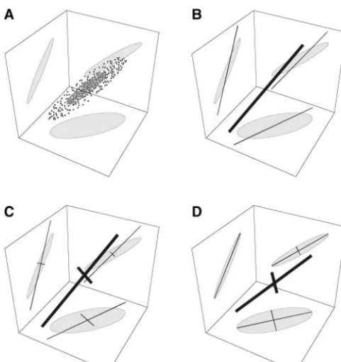
Figure 1 sketches the algorithm in graphical form. genvalues␭Ei for the environmental covariance matrix

Eare defined in an analogous way on the basis of the Step 1 is to estimate the leading genetic and environ-mental principal components. Withktraits, we search environmental PCs, the␺Ei’s.

By rewriting an individual’s breeding value and envi- ak-dimensional space for the first genetic PC,␺A1, and for the first environmental PC,␺E1. The search contin-ronmental deviation in terms of the genetic and

environ-mental PCs, we have just reparameterized Equation 1, ues until we converge on estimates of␺A1and␺E1that optimize the fit (Figure 1B).

swapping one set of variables for another. The central

idea of our scheme is to simplify the estimation problem We can stop at that point or continue by estimating additional PCs. If we choose to go on, step 2 begins by by reducing the number of terms in the sums of

Equa-tions 2 and 3 and therefore the number of parameters searching for the second genetic PC (Figure 1C). We exploit the orthogonality property of PCs by restricting to be estimated. Eigenvalues typically decline rapidly in

step 2, the fit of each successive principal component is conditioned on the PCs that have already been esti-mated. That does not guarantee that the fit is optimized when all the PCs are allowed to vary simultaneously. We do, however, hope to be close to the global optimum at the end of step 2. We therefore perform small rotations on the estimated sets of genetic and environmental PCs and small perturbations on their lengths, now seeking to maximize the fit globally (Figure 1D). These “Givens rotations” are a natural perturbation because they pre-serve the orthogonality of the principal components

(JugaandThompson1992;PinheiroandBates1996).

A rotation is defined by an angle and a pair of axes that determine its equatorial plane. Consider a trial set of m(m ⫺ 1)/2 rotation angles␪ ⫽ {␪12, ␪13, . . . , ␪1m, ␪23, . . .}, where␪ijis the rotation involving the axes de-fined by PCsiandj. Given a set {␺i} of meigenvectors estimated under step 2, we calculate a new set {␺i⬘} that results from the rotation using

␺⬘i ⫽

  

兿

m⫺1

j⫽1

兿

m

k⫽j⫹1

Mjk(␪jk)_



␺i, (6)

Figure1.—Schematic of the search algorithm when fitting

m⫽2 principal components tok⫽3 traits. (A) A scatterplot _{fori⫽ 1, 2, . . . ,m. The quantity in square brackets is} of the data in three dimensions, with the 95% confidence

a matrix that rotates all of the principal components.

ellipses projected onto the bounding planes. (B) Step 1 fits

Mij(␪ij) is a Givens rotation matrix for principal

compo-the first PC with some error. (C) Step 2 fits a second PC in

nentsiandj. It is based on anm-dimensional identity

a direction that is confined to be orthogonal to the first PC.

The result again has some error. (D) Step 3 rotates the two matrix with the following changes: the stth element is

PCs and perturbs their lengths until the overall fit is optimized. _{cos(␪ij) ifs⫽t⫽ior ifs⫽t⫽j, sin(␪ij) ifs⫽i⬍t⫽}

jor ifs⫽ j⬍t⫽ i, and⫺sin(␪ij) ift ⫽i⬍ s⫽jor if t⫽j⬍s⫽i. For example, withm⫽4 principal compo-orthogonal to the first PC, which speeds the search.

nents, the matrix that rotates PCs 1 and 3 through an Likewise, we can choose to search for a second

environ-angle␪13is mental eigenvector. The process is repeated, in each

iteration decreasing by 1 the number of dimensions that must be searched. We are finally left with a set of mA

genetic PCs andmEenvironmental PCs. _M

13(␪13)⫽

    

Cos[␪13] 0 Sin[␪13] 0

0 1 0 0

⫺Sin[␪13] 0 Cos[␪13] 0

0 0 0 1

    

. The search gets easier with each PC because the

num-ber of dimensions of the space in which we search gets smaller. Say that we want to estimate genetic PCi,␺Ai,

Step 3 also requires perturbing the lengths of the having already estimated PCs 1 to i ⫺ 1. We need fit

PCs. That is done by multiplying PCiby 1⫹ ␦i, where onlyk⫺i⫹1 of itskelements because the remaining

the perturbation␦i that optimizes the fit will often be i ⫺ 1 elements are determined by the constraint that

much smaller than 1. In total, step 3 involves searching this next PC must be orthogonal to the previous ones.

among mA(mA ⫺ 1)/2 axes of rotation for the genetic Specifically, let elements 1 to k⫺ i ⫹ 1 of␺Ai be the

PCs,mE(mE⫺1)/2 axes for the environmental PCs,mA elements to be estimated. A bit of algebra based on the

perturbations on the lengths of the genetic PCs, andmE orthogonality constraint then shows that the remaining

perturbations on the lengths of the environmental PCs. elements k⫺i⫹ 2 tokare given by

Figure 1 shows the result of this algorithm in an ideal case where the first two of three PCs are estimated per-fectly. Even with the perfect fit there is variation in the

    

qi,k⫺i⫹2 qi,k⫺i⫹3

⯗ qi,k

    

⫽

    

q1,k⫺i⫹2 q1,k⫺i⫹3 … q1,k q2,k⫺i⫹2 q2,k⫺i⫹3 … q2,k

⯗ ⯗ _{⯗ ⯗}

qi_⫺1,k⫺i⫹2 qi⫺1,k⫺i⫹3 … qi⫺1,k

    

⫺1

    

兺

k⫺i⫹1 j⫽1 q1,jqi,j

兺

k⫺i⫹1

j⫽1 q2,jqi,j ⯗

兺

k⫺i⫹1

j⫽1 qk,jqi,j

    

, _{third dimension, which is not accounted for by the two} PCs. In a real application, further error is introduced because the PCs themselves will not be estimated per-(5) _{fectly. Below we present an example with simulated data}

and further discuss these two sources of error. where for compactness we useqi,jto denote thejth

ele-How many parameters have been estimated in the ment of PC␺Ai.

is a problem that involves (mk⫺m(m⫺1)/2) genetic environmental effects, respectively. The matrix ⌿A is block-diagonal, where blockiis a matrix whose columns parameters. IfmⰆk, the estimation problem increases

approximately linearly with bothmandk. This compares are the firstmA genetic PCs. (If any measurements are missing for individuali, then the corresponding rows very favorably with estimating the unrestricted

covari-ance matrix. That entailsk(k⫹1)/2 parameters, a prob- of this submatrix are deleted.) The matrix⌿Eis formed in the same way using the environmental PCs.

lem that increases roughly as the square ofk.

How do we decide when to stop fitting additional The likelihoodLof a set of parameter values can be written in a variety of ways (reviewed byMeyer1991). principal components? The residual error decreases

with each new principal component that is added. But For the model of Equation 7, a useful form is it does so at the expense of increasing the number of

⫺2 log L⫽const⫹mAlog |A|⫹log |R|⫹log |C|⫹yTP y, parameters in the statistical model: withmPCs already

(8) fitted, estimating another PC addsk ⫺ mparameters.

Several methods are available to determine if the im- _{where |·| denotes a matrix determinant; minimizing this} provement is significant, including the likelihood-ratio _{quantity maximizes the likelihoodL. The first term on} test (Edwards1972) and the Akaike information crite- _{the right is a constant that does not depend on the} rion (AIC;Akaike1973). _{parameters being estimated. The second term is a} func-tion ofA, which is the (numerator) relationship matrix whoseijth element is twice the coefficient of coancestry

ESTIMATING PCs WITH REML

between individuals i and j (e.g., 1/2 for parents and To this point we have focused on an algorithm for _{offspring, 1/4 for half-sibs, etc.). This term is constant} searching parameter space, but not discussed how to _{when the number of genetic PCs being fit is fixed and} evaluate the estimates. REML is a framework that offers _{so needs to be considered only when comparing models} a flexible and powerful approach (Patterson and _{with different degrees of fit (i.e., different values ofmA).}

Thompson1971). Among its strengths are that arbitrary _{In the third term of (8), Ris thekT⫻kTcovariance}

pedigrees can be used, bias from fixed effects (gender, _{matrix for the residual errors ε. It is block-diagonal,} age, environment, etc.) and selection is decreased, and _{with blockRithe diagonal matrix whosejth element is} missing data can be accommodated. Here we follow the _␴2

εj, but with rows and columns that correspond to

miss-argument ofMeyer(1998) to show how REML can be _{ing measurements (if any) deleted. In the fourth term,} applied to the direct estimation of genetic principal _{the matrixC is}

components. A more detailed analysis of the statistical issues is given byMeyerandKirkpatrick(2005).

Read-ers interested in a more general pRead-erspective on the use _C⫽

    

XT_R⫺1_{X X}T_R⫺1_⌿

A XTR⫺1⌿E

⌿T

AR⫺1X ⌿TAR⫺1⌿A⫹A⫺1丢ImA ⌿

T

AR⫺1⌿E

⌿T

ER⫺1X ⌿TER⫺1⌿A ⌿TER⫺1⌿E⫹IN丢ImE

     ,

of likelihood and REML to estimate genetic parameters can consultHarville (1977) andLynchand Walsh

(1998, Chaps. 26 and 27). ₍₉₎

We want to estimate the covariance matrices Gand

where 丢 is the Kronecker (or direct) matrix product

E, which we do by estimating the genetic PCs (the␺Ai)

(Searle1982), andIiis the identity matrix with

dimen-and environmental PCs (the␺Ei). Fitting the model will

sionsi. also give us estimates of the residual error variances

The last term on the right side of Equation 8 involves (the␴2

εi). Our approach is based on the general linear

the matrix model, or “animal model,” of quantitative genetics

(LynchandWalsh1998, Chap. 26). Using Equations _{P ⫽V}⫺1_{⫺ V}⫺1_X(XT_V⫺1_X)⫺_XT_V⫺1_{, (10)}

1 and 3, the data for all of the individuals can be written

where⫺is a generalized matrix inverse (Searle1982). as the mixed model:

V⫽Var[y] is a block-structured matrix whoseijth block

y⫽X␤⫹ ⌿A␣⫹⌿E␥ ⫹ε. (7) _{describes the expected covariance in measurements} be-tween individualsiandj,

On the left is the vectoryofkTobservations, formed by

concatenating the corresponding vectors for individu- _V

ij⫽ Aij⌿Ai⌿TAj⫹ ␦ij⌿Ei⌿TEi⫹ ␦ijRi, (11) als. On the right, the vectors␣(the breeding values for

the genetic PCs),␥(the deviations for the environmen- where␦ij ⫽1 ifi⫽jand is 0 otherwise.

Equations 8–11 tell us how to calculate the restricted tal PCs), andε(the residual errors) are formed in the

same way. The first term on the right side is the vector likelihood L. REML estimates for the parameters (the genetic and environmental PCs and the residual error) of mean effects, which is the product of the design

matrix X and the vector ␤ of unknown fixed effects. are those values that maximizeL. In practice, the esti-mates are found numerically. Evaluating the equations REML is based on a transformation that removes the

matrices. In animal breeding applications, for example, is simple:G(x1,x2) andE(x1,x2) are just the additive genetic and environmental covariances for the trait between ages it is not unusual for the calculations to involve solving

millions of simultaneous equations (Misztalet al.2000; x1andx2. Like the genetic covariance matrixGfor multi-variate traits, the covariance functionGdetermines how FV

Schaeffer2004). Great effort has gone into developing

efficient algorithms, however, with the result that it is traits respond to selection (Kirkpatrick andHeckman

1989;GomulkiewiczandBeder1996). The relations now feasible to find REML estimates for even very large

data sets.MeyerandKirkpatrick(2005) discuss some between the covariance functions and the eigenfunc-tions are given by the analogs of Equaeigenfunc-tions 2:

of the numerical issues involved with the direct-estima-tion approach in more detail.

G(x1,x2)⫽

兺

mA

i⫽1

␺Ai(x1)␺Ai(x2), E(x1,x2)⫽

兺

mE

i⫽1

␺Ei(x1)␺Ei(x2).

(13)

FUNCTION-VALUED TRAITS

In general, decomposing a covariance function into As mentioned in the Introduction, traits like growth _{a sum of eigenfunctions requires an infinite number of} trajectories and reaction norms arefunction valued(FV). _{terms, in which case the limits of the sums in (13) and} Because the value of the character is a function of a _{(14) are infinity. In practice, however, experience shows} continuouscontrol variable(such as age or temperature), _{that most genetic and phenotypic variation is associated} we can view these traits as consisting of an infinite num- _{with the first two or three PCs (e.g.,Kirkpatricket al.} ber of dimensions. The natural way to describe variation _{1990, 1994; Kirkpatrick and Lofsvold1992). Thus} in such traits is with a covariance function whose value _{our approach once again is to approximate the} covari-gives the covariance of the character between any pair _{ance structure by truncating the sums, using values of} of values for the control variable (KirkpatrickandHeck- _m

AandmEthat are as small as possible but that still give

man1989). Because function-valued traits have higher _{an adequate description of the population.}

dimensionality than multivariate traits, the need to find _{The new issue raised by function-valued traits is how} efficient descriptions of variation for FV traits is even _{to represent the eigenfunctions. If we do not place any} more acute. The concepts developed above for multivar- _{constraint on their form, estimating each of them would} iate phenotypes extend in a natural way to the FV setting _{involve searching an infinite-dimensional space.} Fortu-with only minor changes. In what follows, we talk about _{nately, biological covariance functions and their} eigen-age as the control variable, as when studying growth curves, _{functions tend to be smooth. That means that the} eigen-but the control variable could as well be an environmental _{functions can be approximated in a simple way. The} variable (e.g., temperature) or a spatial coordinate. _{key is to write each of them as a weighted sum of a set}

We begin the discussion of function-valued traits by _{of basis functions, {φj(·)}:} showing how they can be represented using principal

components in a way that is completely analogous with _␺Aj(x)⫽

_兺

k_A

i⫽1

φi(x)CAij, ␺Ej(x)⫽

兺

k_E

i⫽1

φi(x)CEij (14) the multivariate case. We then show how the genetic

parameters can be estimated using the search algorithm _{(KirkpatrickandHeckman1989). When suitable basis} and via REML. _{functions are chosen, experience shows that very good}

Representing FV traits with PCs: Measurements are _{approximations to the eigenfunctions are often achieved} taken on each individual at a set of ages, and the number _{with a small number of terms, say three or four.} of measurements and the ages may differ between indi- _{A very broad range of basis functions could be used} viduals. The additive genetic and environmental contri- _{to represent the eigenfunctions. The computations are} butions to thejth measurement for individualican be _{simplified, however, if we use orthogonal functions that} written with a minor modification of Equation 3, _{have been scaled to have unit norm over the range of} the control variablex, and we assume that the {φi} have aij ⫽

兺

mA

l⫽1

␣il␺Al(xij), eij⫽

兺

mE

l⫽1

␥il␺El(xij), (12) those properties in what follows. One natural choice for the basis functions is Legendre polynomials (see

Kirk-patrick et al. 1990; Meyer 1998). Estimates for the

wherexijis the age at which that measurement was taken.

eigenfunctions are then polynomials of degree k⫺ 1. Comparing these expressions with (3), we see that the

An alternative possibility for the basis function is splines. genetic and environmental eigenvectors,␺Aand␺E, have

The additive genetic variances for the genetic princi-been replaced by the genetic and environmental

eigen-pal components can be written in terms of the weights functions, ␺A(·) and ␺E(·). These eigenfunctions act as

that appear in Equation 14 : the principal components of the FV setting. Like their

multivariate analogs, they can be used to describe

varia-␭Ai⫽

兺

k_A

j⫽1 C2

Aij (15)

tion in a population.

The genetic and covariance matrices of the

an FV trait are determined by the vector of weightsCAi sions in which to search. To do that, we use the algorithm described earlier. Specifically, replace␺Aiin Equation 5 in the same way they are by the genetic eigenvector␺Ai

in the MV setting. withCAi, and replace␺EiwithCEi, whereCAiandCEiare respectively theith columns of the matricesCAandCE. Our approximation for function-valued traits

there-fore works on two levels. First, the covariance functions We finish with step 3, the final optimization that rotates and perturbs the lengths of the vectors that compose are approximated by reconstructing them using only the

firstmprincipal components (eigenfunctions). Second, the columns ofCAandCE, just as in the multivariate case.

Estimation with REML:With a function-valued trait, the principal components themselves are approximated

by functions with onlykdegrees of freedom (for exam- the aim is to estimate the covariance functionsG(·,·) andE(·,·). The approach is again based on estimating ple, polynomials of degreek⫺1). We might find, for

ex-ample, that the data are well described by two principal the genetic and environmental PCs, which are now the eigenfunctions␺Ai(·) and␺Ei(·). Fitting the model also components (m⫽2), each of which is a cubic (k⫽4).

We can now describe an individual’s breeding value gives estimates of the residual error variances.

The calculations described earlier for the MV setting in terms of genetic principal components. Putting

to-gether Equations 12 and 14, we see thatai, the vector carry over to FV traits with only trivial changes. In Equa-tions 7–11, the matrix⌿Aiis replaced by⌽iCA, and the of individuali’s breeding values for the trait at the ages

at which it was measured, can be written in terms of␣i, matrix⌿Eiis replaced by⌽iCE. The last thing needed is a model for the residual error. The residual error matrix its vector of its breeding values for the genetic principal

components, for individualiis diagonal with elements [Ri]jj⫽ ␴2

ε(xij),

where␴2

ε(x) is the residual (temporary environmental)

ai⫽⌽iCA␣i, (16)

error at agex. A reasonable approach is to assume that this function can be represented by a smooth function where [⌽i]jk⫽φk(xij).CAis thekA⫻mAmatrix of

coeffi-cients that appear in Equation 14. [This matrix is related like a polynomial or spline, in which case the coefficients of that function are included among the parameters we to the coefficient matrixCGofKirkpatricket al.(1990)

viaCG⫽ CA CTA.] Similarly, the environmental compo- seek to estimate (seeMeyer2001). nent of the phenotype can be writtenei⫽⌽iCE␥i.

Be-cause we have chosen to represent these components in

AN EXAMPLE

turn as sums of orthogonal basis functions, the columns

ofCAare mutually orthogonal, as are the columns ofCE. This section illustrates the direct estimation approach We have now succeeded in representing a finite num- _{and our algorithm for fitting PCs. The numerical} exam-ber of phenotypic observations in terms of sums of or- _{ple uses likelihood to estimate the PCs and the} covari-thogonal basis functions. Estimates of the covariance _{ance function of a function-valued trait. For simplicity,} functions are found by optimizing the fit of the coeffi- _{we use a phenotypic example in which the aim is simply} cient matricesCAandCE, using the statistical framework _{to estimate the phenotypic covariance function using full} of our choice. Those matrices then give us estimates for _{maximum likelihood. Meyer and Kirkpatrick (2005)} the PCs (Equation 14), their eigenvalues (Equation 15), _{analyze a genetic example using restricted maximum} and the covariance functions (Equation 13). As in the MV _likelihood.

case, the covariance function is guaranteed to be posi- _{The simulated data:The covariance function is taken} tive-definite. In the next two subsections we show how _{from the numerical example from Kirkpatrick et al.} optimizing the estimates can be accomplished using our _{(1990), which in turn is based on a study of growth in} search algorithm and the REML estimation framework. _{mice byRiskaet al.(1984). The covariance function is}

Searching for the PCs of an FV trait:The algorithm

P(a1,a2)⫽ 5655⫺ 4256(a1⫹a2)⫹642(a21⫹a22) described earlier in the MV setting now carries over

di-rectly if we visualize the columns of the coefficient ma- _{⫹ 3462a}

1a2⫺ 530(a1a22⫹ a12a2)⫹81.6a21a22 tricesCAandCEas the analogs of the eigenvectors␺Aand ₍₁₇₎ ␺E(respectively) from the multivariate case. In brief, we

for 2ⱕa1,a2ⱕ 4. The function is shown in Figure 2. search sequentially for the vectors that make up the

col-Because this function is quadratic, it has only three umns ofCAandCEin just the same way that we searched

nonzero PCs, which are shown in Figure 3. They are in the multivariate setting for the eigenvectors␺A and

␺E. Step 1 involves searching for themAelements of the _{␺1⫽43.87⫺ 45.89a⫹7.269a}2_, first column ofCAand themEelements of the first column

␺2⫽57.15⫺ 33.39a⫹4.64a2_, ofCEthat optimize the fit. These give estimates of the

first genetic and environmental PCs (eigenfunctions). _␺3⫽

21.53⫺ 15.52a⫹2.688a2_{. (18)} In step 2, we search sequentially for additional columns

ofCA andCE, which give estimates of subsequent PCs. (These differ from the corresponding equations in

Kirkpatricket al.1990, p. 984, because here age is on

We can exploit the fact that the columns of these

Figure2.—The covariance function used in the numerical example.

are defined to be equal to the square root of the corre-sponding eigenvalues.) The eigenvalues are␭1⫽1361, ␭2 ⫽24.54, and␭3⫽1.535.

The aim is to estimate the phenotypic covariance functionPby fittingm⫽ 1, 2, and 3 principal compo-nents. For each replicate, we simulated a population of 100 individuals, each measured atk⫽5 equally spaced ages. The covariance matrix for the traits was deter-mined by evaluating Equation 17 on a 5 ⫻5 lattice of points. An individual’s phenotype was simulated as a vector of five measurements sampled from the corre-sponding multivariate normal distribution with mean

zero. To each of these measurements we added an i.i.d. _{Figure 3.—The three principal components} (eigenfunc-“temporary environmental error” (or measurement er- tions) of the covariance function for the numerical example. The actual PCs are the thick solid curves, and typical estimates

ror) term with variance ␴2

ε⫽ 625, which corresponds

are shown as dashed curves.

to between 43 and 59% of the total variance, depending on the point in the covariance function. We fit one, two, and three PCs to each sample of 100 individuals via

We evaluated the accuracy with which the individual full likelihood (because the model has no fixed effects).

principal components were estimated in two ways. A PC The likelihood was maximized using the derivative-free

is a vector quantified by a direction and a length (or simplex algorithm (NelderandMead1965). For each

norm). (This holds equally for function-valued traits, degree of fit (that is, value ofm), we calculated the

cor-where the “direction” is reflected by the shape of the responding estimate for the covariance function using

PC, or eigenfunction.) A natural measure of the error Equation 13. We also estimated the full 5⫻5 covariance

in the estimated direction is the angle between the esti-matrix, which is equivalent to a multivariate analysis

mate and the true PC. For the multivariate case, that is that ignores the ordering of the ages at which the

mea-surements were taken. This procedure was repeated for

␪i⫽arccos

  

␺T i␺ˆi |␺| |␺ˆ|

  

, (20)

10,000 replicates.

Measuring the accuracy of the estimates:We evaluated

our estimation approach in several ways. Our first mea- _{where |·| denotes norms of vectors. [This relation} fol-sure is the average proportional error in the overall _{lows from the fact that the inner product of two vectors} estimate of the covariance function reconstructed from _{with unit norm is equal to the cosine of the angle}

be-the PCs, _{tween them (Strang 1976).] For the function-valued}

case, the analogous expression is

ε(P)⫽

冮冮

x_max

x_min

|Pˆ(x1,x2)⫺P(x1,x2)| P(x1,x2)

d_x1d_x2/(xmax⫺ xmin)2,

␪i⫽arccos

冤

冮

xmax

xmin

␺i(x)(␺ˆ)i(x)dx

/

冪冢

冮

xmax

xmin

␺2 i(x)dx

冣冢

冮

xmax

xmin

␺ˆ2 i(x)dx

冣冥

(19)

where the hat denotes an estimate, and the ages range

from xmin⫽ 2 to xmax ⫽ 4. We calculated the integrals ⫽_arccos

 

CT iCˆi

|Ci||Cˆi|

  

, ₍₂₁₎

whereCiis the vector of coefficients for PCithat appears in Equations 14 and 15. If the direction (or shape, in the FV context) of an estimated PC is perfectly aligned with the population value, then␪ is the ideal 0⬚, while if the estimate is a perfect failure (that is, the estimate is orthogonal to the true PC), then␪ ⫽90⬚.

Our second measure for the accuracy with which the PCs were estimated is the relative error in an estimate of eigenvalue i (which is the square of the norm, or length, of PCi):

ε(␭i)⫽|␭ˆi⫺ ␭i|/␭i. (22)

This measure is zero when the magnitude of the eigen-value is estimated perfectly and otherwise is positive. We quantified the bias in estimate of the eigenvalue as

bias(␭i)⫽(␭ˆi⫺ ␭i)/␭i. (23)

This measure is zero when the eigenvalue is estimated with no bias, is negative when it is underestimated on aver-age, and is positive when it is overestimated on average. Finally, we quantified the relative error in the esti-mates of the temporary environmental variance using a statistic analogous to what we used for the eigenvalues:

ε(␴2

ε)⫽ |␴ˆ2ε⫺ ␴2ε|/␴2ε. (24)

Results: Table 1 shows the simulation results. The direct estimation approach does well in estimating the overall covariance function: on average, the covariances are estimated with an error of 15%. This is encouraging in view of the facts that the data sets consisted of only 100 individuals and the variance contributed by surement error was roughly as large as that of the mea-surements themselves.

A striking result is that the accuracy in estimating the covariance function when two or three PCs are fit is no better than when just one PC is estimated: neitherε(␪1) norε(␭1) changed substantially when different numbers of PCs were fit. The reason becomes clear when we look at the estimation errors for the PCs (Figure 3). The first PC is consistently well estimated. The average error in estimating its shape is trivial:ε(␪1)⫽2.7⬚. The error in es-timating the first eigenvalue,ε(␭1), is greater: on average the estimate is off by 14%. The bias for that eigenvalue, however, is extremely small. On average it is underesti-mated, but by⬍1% of its true value. This contrasts with standard multivariate methods, which can produce sub-stantial upward biases in estimates of the leading eigen-value (HayesandHill1981).

The situation is quite different for the second and subsequent PCs. The shape (direction) of the second PC is poorly estimated, with an error of 28⬚, and esti-mates for the second eigenvalue are on average 83–90% away from their true values. The third eigenfunction fares even worse: the error in the shape is 29⬚, and the average error in the estimate of␭3is 190%. But because these PCs contribute so little to the total variation, these

TABLE 1 Errors in the estimates b ased on fi tting m ⫽ 1, 2, and 3 p rincipal components to simulated phenotypic data sets, each consisting o f 1 00 individuals (see text for details) PC1 PC2 PC3 m ε ( P ) ε ( ␭1 ) B ias( ␭1 ) ε ( ␪1 ) ε ( ␭2 ) B ias( ␭2 ) ε ( ␪2 ) ε ( ␭3 ) Bia s( ␭3 ) ε ( ␪3 ) ε ( ␴

2)ε

DISCUSSION

errors have almost no impact on the accuracy of the

overall estimate of the covariance function. _{The point of departure for this article is the simple} How do the results depend on the number of mea- _{observation that covariance matrices and covariance} surements taken on each individual? Not surprisingly, _{functions can be estimated directly in terms of a small} the accuracy of the estimate for the leading PC improves _{number of principal components. Several benefits flow} as the number of ages measured increases. As a result, _{from this strategy. The data are used efficiently in the} the entire covariance function is better estimated. Com- _{sense that the maximum amount of variation is} ex-paring results for five ages (Table 1) with those for nine _{plained with the smallest number of parameters. This} ages (not shown), the estimation error in the overall co- _{reduction should speed calculations and lead to greater} variance function decreases by 11%. The error in esti- _{numerical stability of the estimates. The covariance} ma-mating the leading eigenvalue declines by 10%, and the _{trix (or function) estimated by the direct method is} guar-error in the estimate of the direction of PC1 by 18%. _{anteed to be positive semidefinite. Last, estimation biases} These improvements may seem modest, given that the _{for the leading eigenvalues, which have long been} recog-amount of data is almost doubled. But this situation is _{nized as a problem in classical estimation approaches,} ap-far better than what we would see with a conventional _{pear to be reduced substantially. These last two points} ob-multivariate analysis. There, the accuracy of the estimates _{viate the need for heuristic corrections to estimates of} can actually decline because the number of parameters _{covariance matrices, for example, the “bending” method} being estimated increases so rapidly with the number _{proposed byHayesandHill(1981). Some of the} advan-of traits measured (SalesandHill1976a,b). _{tages of working with genetic PCs have been recognized} It is also interesting to compare these results with a _{previously (Misztalet al.2000;Nobreet al.2002), but it} standard multivariate analysis of the same data. In effect, _{seems they have not yet been exploited systematically.} the MV approach discards all information about the _{We have seen that the orthogonality of PCs can be} ages at which the measurements were taken. The aver- _{exploited in an algorithm to estimate the covariance} age relative error in estimating the 5 ⫻ 5 covariance structure. Pinheiroand Bates (1996) compared the matrix is 20%, which is worse than the error when we efficiency of the Givens rotations (which is the third estimate only a single PC but make use of the function- component of our algorithm) with four other parame-valued nature of the data (15%; see Table 1). The rela- terizations used for estimating covariance matrices from tive error in the estimate of the first eigenvalue is very phenotypic data. They found that other parameteriza-similar for the standard MV approach and our new tions are often faster, largely because of the computa-approach [ε(␭1)⫽0.14 for both], but the MV approach tional expense of the calculations involving the rota-also estimates the direction of the leading principal tions. In large genetic analyses, however, this may not be component with greater error than the FV approach a concern because calculating the likelihood itself will does (5.5⬚vs.2.7⬚). These results reinforce the impres- typically be a much larger part of the problem. A sepa-sion that combining the FV and the direct estimation rate issue is whether likelihood surfaces for genetic pa-approaches makes efficient use of the data. rameters under our parameterization are conducive to Bias in estimates of the leading eigenvalues is reduced numerical search.MeyerandKirkpatrick(2005) ana-by the new method. We used the simulated data to es- lyzed a genetic example and found that the direct esti-timate the leading eigenvalue using the standard MV mation approach seems to be quite efficient in that con-approach, that is, by calculating the eigenvalues from text also. Extensive simulations will be needed, however, the estimated covariance matrix. The estimate is typi- to determine the robustness of the approach in general. cally biased upward, as expected from the arguments of One potentially useful application of the direct PC

HayesandHill(1981), on average by 3.8%. But when approach is in studies of the evolution of the additive

the direct estimation method is used, bias is much re- genetic variance-covariance structure, a topic of emerg-duced. Depending on the number of PCs estimated, ing interest in evolutionary genetics. A variety of statisti-bias under the direct estimation method is between cal tools have been developed to compare covariance three and nine times smaller than that under the classic matrices (reviewed byHouleet al.2002;Steppanet al.

MV approach. 2002). Among them are methods that focus on

proach contributes. Further work is needed on several some applications. Evolutionary biologists would like to know the degree to which patterns of genetic variation issues, for example, to determine how the choice of the

number of PCs estimated affects these analyses. may constrain the potential for adaptation (Maynard

Smithet al.1985). Function-valued traits are a

particu-The direct PC approach may be most useful with

function-valued traits. The additive genetic covariance larly interesting context in which to study this problem because there are in principle an infinite number of function plays a central role in determining how FV

traits respond to natural and artificial selection (Kirk- dimensions to which organisms must adapt (

Kirkpat-rickandLofsvold1992). Our approach of extracting

patrick and Heckman 1989; Kirkpatrick 1993;

Gomulkiewicz and Beder 1996; Kirkpatrick and only the major PCs is poorly suited to this kind of

prob-lem because it will often discard information about

phe-Bataillon1999). Consequently, estimation and

analy-sis of covariance functions is rapidly expanding in both notypic dimensions for which there is a small but non-zero amount of genetic variation. By neglecting these evolutionary genetics and applied animal breeding (

Jaf-fre´zicandPletcher2000;Misztalet al.2000;King- dimensions, we might be falsely led to believe there is

no heritable variation available for adaptation when in

solveret al.2001;Schaeffer2004). Estimates of

covari-ance functions are sensitive to error, however, and so fact there is.

Some kinds of traits do not fall into either the multi-there is substantial interest in developing methods that

are fast, make efficient use of the data, and are numeri- variate or function-valued cases we discussed above. We might be interested in a set of several traits that change cally stable (Jaffre´zic and Pletcher 2000; van der

Werf2002). with age, for example, or in a trait that varies as a func-tion of more than one continuous control variable (for Two major families of methods to estimate covariance

functions are currently in use. The first, which is nonpar- example, age and environment). The direct estimation approach can be extended to these more complex kinds ametric in spirit, represents the covariance function in

terms of flexible basis functions such as polynomials. of phenotypes. This is an attractive idea because the number of parameters to be estimated is otherwise very The earliest approach fit polynomials to a covariance

matrix that had been previously estimated for a fixed set large (Schaeffer2004).

There has recently been much interest in function-of ages (Kirkpatricket al.1990, 1994). An important

advance was the introduction of the method of random valued traits among statisticians working in areas out-side of quantitative genetics.RiceandSilverman(1991) regression, which escapes the need for the covariance

matrix by fitting a set of basis functions to the observa- introduced a nonparametric approach in which obser-vations on individuals were fit with splines, and the PCs tions for each individual (Schaeffer and Dekkers

1994; Meyer and Hill 1997; Meyer 1998). Random were derived from them. Their approach has been ex-panded and generalized in several respects (Ramsayand regression has been widely implemented using

poly-nomials as the basis functions (Schaeffer2004), but Silverman1997, 2002). Some of the developments par-allel those made independently in quantitative genet-other basis functions such as splines have also been

used (White et al. 1999; Torres 2001). Splines are ics, for example, the use of random regressions (James

et al. 2000). There are, however, basic differences be-numerically better behaved than polynomials, but have

the drawback that they require fitting a larger number tween these phenotypic analyses and those in quantita-tive genetics. Major goals of quantitaquantita-tive genetics are of parameters and so can become unwieldy with very

large data sets. to partition variation into heritable and nonheritable components and to estimate the breeding values of indi-The second family of methods begins with the

as-sumption that the covariance function takes a simple viduals. Those goals motivate the standard assumption of quantitative genetics that variance components are parametric form (e.g.,PletcherandGeyer1999;

Jaf-fre´zicet al.2003). This constraint reduces the number normally distributed. In contrast, many phenotypic

ap-plications can afford to take more general nonparamet-of parameters and so makes the results less sensitive to

estimation error (Jaffre´zic and Pletcher 2000). A ric approaches (Ramsay andSilverman 1997, 2002). Nevertheless, the direct PC approach developed here drawback of this approach is that there is often no strong

biological justification for any particular functional may also find uses in the analysis of phenotypic data. form. If an inappropriate choice is made, then estimates _{This work was supported by grant BFGEN.100 of Meat and Livestock} of genetic parameters will be biased. Australia (to K.M.) and grants DEB-9973221 and EF-0328594 from the National Science Foundation and NER/A/S/2002/00857 from the

The direct estimation method proposed in this article

Natural Environment Research Council (to M.K.).

may have some of the advantages of both families of methods. It makes no prior assumption about the form of the covariance function, but involves many fewer

LITERATURE CITED

parameters than the standard random regression

meth-ods. The reduction may make it feasible to use more Akaike, H., 1973 Information theory and an extension of the maxi-mum likelihood principle, pp. 267–281 inThe Second International

complex models, for example, using splines rather than

Symposium on Information Theory, edited by B. N. Petrov and

polynomials to estimate the eigenfunctions. _{F.Csaki. Akad. Kiado`, Budapest.}

Atchley, W. R., andJ. J. Rutledge, 1980 Genetic components of

size and shape. I. Dynamics of components of phenotypic variabil- Meyer, K., 1998 Estimating covariance functions for longitudinal data using a random regression model. Genet. Sel. Evol.30:221–240. ity and covariability during ontogeny in the laboratory rat.

Evolu-Meyer, K., 2001 Estimating genetic covariance functions assuming

tion34:1161–1173.

a parametric correlation structure for environmental effects. Chase, K., D. R. Carrier, F. R. Adler, T. Jarvik, E. A. Ostrander

Genet. Sel. Evol.33:557–585. et al., 2002 Genetic basis for systems of skeletal quantitative

Meyer, K., andW. G. Hill, 1997 Estimation of genetic and

pheno-traits: principal component analysis of the canid skeleton. Proc.

typic covariance functions for longitudinal data by restricted max-Natl. Acad. Sci. USA99:9930–9935.

imum likelihood. Livest. Prod. Sci.47:185–200.

Edwards, A. W. F., 1972 Likelihood: An Account of the Statistical Concept

Meyer, K., andM. Kirkpatrick, 2005 Restricted maximum

likeli-of Likelihood and Its Application to Scientific Inference.Cambridge

hood estimation of genetic principal components and smoothed University Press, Cambridge, UK.

covariance matrices. Genet. Sel. Evol.36(in press).

Falconer, D. S., andT. F. C. Mackay, 1996 Introduction to

Quantita-Misztal, I., T. Strabel, J. Jamrozik, E. A. Ma¨ntysaariandT. H. E.

tive Genetics, Ed. 4. Longman, London.

Meuwissen, 2000 Strategies for estimating the parameters

Flury, B. D., 1988 Common Principal Components and Related

Multivari-needed for different test-day models. J. Dairy Sci.83:1125–1134. ate Models. Wiley, New York.

Morrison, D. F., 1976 Multivariate Statistical Methods. McGraw-Hill,

Gomulkiewicz, R., andJ. H. Beder, 1996 The selection gradient

New York. of an infinite-dimensional trait. Soc. Ind. Appl. Math. J. Appl.

Nelder, J. A., andR. Mead, 1965 A simplex method for function

Math.56:509–523.

minimization. Comput. J.7:147–151.

Harville, D. A., 1977 Maximum likelihood approaches to variance

Nobre, P. R. C., I. Misztal, S. Tsuruta, J. K. Bertrand, L. O. C. component estimation and to related problems. J. Am. Stat. Assoc.

Silvaet al., 2002 Genetic evaluation of growth in beef cattle

72:320–338.

with a random regression model. Seventh World Congress on

Hayes, J. F., and W. G. Hill, 1981 Modification of estimates of

Genetics Applied to Livestock Production, INRA, Castanet-Tolosan, parameters in the construction of genetic selection indices

France, Communication 20.10. (‘bending’). Biometrics37:483–493.

Patterson, H. D., andR. Thompson, 1971 Recovery of inter-block

Hill, W. G., andR. Thompson, 1978 Probabilities of non-positive

information when block sizes are unequal. Biometrika58:545–554. definite between-group or genetic covariance matrices.

Biomet-Phillips, P. C., andS. J. Arnold, 1999 Hierarchical comparison of

rics34:429–439.

genetic variance-covariance matrices. I. Using the Flury hierarchy.

Houle, D., J. MezeyandP. Galpern, 2002 Interpretation of results

Evolution53:1506–1515. of common principal components analysis. Evolution56:433–440.

Pinheiro, J. C., andD. M. Bates, 1996 Unconstrained

parameteriza-Jaffre´zic, F., andS. D. Pletcher, 2000 Statistical models for

esti-tions for variance-covariance matrices. Stat. Comput.6:289–296. mating the genetic basis of repeated measures and other

function-Pletcher, S. D., andC. J. Geyer, 1999 The genetic analysis of

age-valued traits. Genetics156:913–922.

dependent traits: modeling the character process. Genetics153:

Jaffre´zic, F., R. ThompsonandW. G. Hill, 2003 Structured

antede-825–835. pendence models for genetic analysis of repeated measures on

Ramsay, J. O., andB. W. Silverman, 1997 Functional Data Analysis.

multiple quantitative traits. Genet. Res.82:55–65.

Springer, New York.

James, G. M., T. J. HastieandC. A. Sugar, 2000 Principal

compo-Ramsay, J. O., andB. W. Silverman, 2002 Applied Functional Data

nent models for sparse functional data. Biometrika87:587–602.

Analysis. Springer, New York.

Juga, J., andR. Thompson, 1992 A derivative-free algorithm to

esti-Rice, J. A., andB. W. Silverman, 1991 Estimating the mean and

co-mate bivariate (co)-variance components using canonical

trans-variance structure nonparametrically when the data are curves. formations and estimated rotations. Acta Agric. Scand. Sect. A

J. R. Stat. Soc. B53:233–243. Anim. Sci.42:191–197.

Riska, B., W. R. AtchleyandJ. J. Rutledge, 1984 A genetic analysis

Kingsolver, J. G., R. GomulkiewiczandP. A. Carter, 2001

Varia-of targeted growth in mice. Genetics107:79–101. tion, selection and evolution of function-valued traits. Genetica

Sales, J., andW. G. Hill, 1976a Effect of sampling errors on

effi-112–113:87–104.

ciency of selection indices. 1. Use of information from relatives

Kirkpatrick, M., 1993 Evolution of size and growth in fisheries

for single trait improvement. Anim. Prod.22:1–17. and other harvested natural populations, pp. 145–154 in The

Sales, J., andW. G. Hill, 1976b Effect of sampling errors on

effi-Exploitation of Evolving Resources(Lecture Notes in Biomathematics

ciency of selection indices. 2. Use of information on associated 99), edited by K.Stokes, J. M.McGladeand R.Law.Springer- _{traits for improvement of a single important trait. Anim. Prod.} Verlag, Berlin.

23:1–14.

Kirkpatrick, M., and T. Bataillon, 1999 Artificial selection on

Schaeffer, L. R., 2004 Application of random regression models

phenotypically plastic traits. Genet. Res.74:265–270. _{in animal breeding. Livest. Prod. Sci.86:35–45.}

Kirkpatrick, M., andN. Heckman, 1989 A quantitative genetic _{Schaeffer, L. R., andJ. C. M. Dekkers, 1994 Random regression}

model for growth, shape, reaction norms, and other infinite- _{in animal models for test-day production in dairy cattle.} Proceed-dimensional characters. J. Math. Biol.27:429–450. _{ings of the 5th World Congress on Genetics Applied to Livestock}

Kirkpatrick, M., andD. Lofsvold, 1992 Measuring selection and _{Production, Guelph, Ontario, Canada, Vol. 18, pp. 443–446.}

constraint in the evolution of growth. Evolution46:954–971. _{Searle, S. R., 1982 Matrix Algebra Useful for Statistics. Wiley, New York.}

Kirkpatrick, M., D. LofsvoldandM. Bulmer, 1990 Analysis of _{Steppan, S. J., P. C. Phillipsand D. Houle, 2002 Comparative}

the inheritance, selection, and evolution of growth trajectories. _{quantitative genetics: evolution of theGmatrix. Trends Ecol. Evol.}

Genetics124:979–993. _{17:320–327.}

Kirkpatrick, M., W. G. HillandR. Thompson, 1994 Estimating the _{Strang, G., 1976 Linear Algebra and Its Applications. Academic Press,}

covariance structure of traits during growth and aging, illustrated _{New York.}

with lactations in dairy cattle. Genet. Res.64:57–69. _{Torres, R. A. A., 2001 Markov chain Monte Carlo methods for}

estimat-Lynch, M., andJ. B. Walsh, 1998 Genetics and Analysis of Quantitative _{ing the covariance structure of longitudinal data: an application to}

Traits. Sinauer Associates, Sunderland, MA. _{dairy cattle. Ph.D. Thesis, Cornell University, Ithaca, NY.}

Maynard Smith, J., R. Burian, S. Kauffman, P. Alberch, J. Camp- _{van der Werf, J. H. J., 2002 Optimizing selection for traits along}

bellet al., 1985 Developmental constraints and evolution. Q. _{trajectories. Seventh World Congress on Genetics Applied to}

Live-Rev. Biol.60:265–287. _{stock Production, INRA, Castanet-Tolosan, France,}

Communica-Meyer, K., 1985 Maximum likelihood estimation of variance compo- _{tion 16.07.}

nents for a multivariate mixed model with equal design matrices. _{White, I. M. S., R. ThompsonandS. Brotherstone, 1999 Genetic}

Biometrics41:153–165. _{and environmental smoothing of lactation curves with cubic splines.}

Meyer, K., 1991 Estimating variances and covariances for multivari- _{J. Dairy Sci.82:632–638.}

ate animal models by restricted maximum likelihood. Genet. Sel.