Modelling polycrystalline microstructures using polygonal finite element

MODELLING POLYCRYSTALLINE MICROSTRUCTURES USING

POLYGONAL FINITE ELEMENT

S. Chakraborty, S. Singh, D. Roy Mahapatra

Department of Aerospace Engineering, Indian Institute of Science, Bangalore, INDIA-560012 E-mail of corresponding author: [email protected]

ABSTRACT

In this paper we employ numerical schemes to optimally integrate the stiffness terms on polygonal shaped finite elements. This powerful method involving polygonal shaped finite elements has several advantages in context of material microstructure modeling as compared to explicit meshing of microstructure by standard quadrilateral finite elements. First we discuss the theoretical background behind the optimal numerical schemes to get the optimal integration points for any polygonal domain. Then optimum integration points are obtained for quadrilateral, pentagonal and hexagonal element with structured mesh. Next, this optimum integration points are used to compute the strain-energy, considering the material as polycrystalline in nature where the material axis of each grain is rotated according to crystallographic properties. The performance of the new scheme is verified with commercial finite element packages by explicitly meshing each polygonal crystal treated as a sub-domain with material property varying from one sub-domain to another according to the crystallographic orientation. Results are verified considering cantilever beam without crack using the newly developed Polygonal Finite Element (PFEM) framework and the same domain with crack using eXtended Finite Element (XFEM) framework.

INTRODUCTION

Finite Element Method (FEM) is a powerful numerical method to solve partial differential equation and it has been used widely in the industry. But almost all commercial FEM packages use either triangulation or quadrilateral element to discretize the domain. In problems involving finite element modeling of microstructure of polycrystalline materials, typically either a continuum level elasto-plastic constitutive model is used or each polygonal grain is explicitly discretized into triangles or quadrilaterals with grain level material details. This is done mainly because of the non-availability of any better quadrature rule for numerical integration of terms in the finite element equations defined over polygonal domains (typical grains being of polygons with more than four sides). In case of microstructure modeling it appears to be most convenient to consider each grain as an element itself, which requires polygonal type element. Other than polycrystal microstructure problem, in several other problems involving complex geometry and ill-posed aspect ratio or shape of object, it is often easier to discretize a complicated geometry using polygonal element.

FINITE ELEMENT FORMULATION FOR LINIER STATIC ELASTICITY PROBLEM

The governing differential equation for two-dimensional linear elasticity problem defined in the domain Ω bounded by Γ is given by

0 in

T

s

σ

b

∇

+ =

Ω

(1)

where

σ

is the stress tensor and b is the vector of external forces. The boundary conditions can be expressed as

u t

on

on

T

u

u

n

σ

t

=

Γ

=

Γ

(2)

where

u

=

(

u u

x

,

y

)

is the prescribed displacement vector on the essential boundary

Γ

_u and

t

=

( ,

t t

x y

)

is the

prescribed traction vector on the natural boundary

Γ

t;

n

is the unit outward normal vector. The weak form

becomes

(

s

) ( )

s

( )

( )

0

T _{T T}

u

D

u d

u

bd

u

td

δ

δ

δ

Ω Ω Γ

∇

∇

Ω −

Ω −

Γ =

where

u

_{is the trial function which satisfies the essential boundary condition on}

Γ

u and

D

is the constitutive

matrix. The finite element method uses the following trial function

h

1

u ( )

N ( )

p

n

i i

i

x

x u

=

=

∑

(4)

where

n

_p is the total number of nodes in the mesh and

u

i are the degrees of associated with node

i

. By

substituting the trial function in the week form and invoking the arbitrariness of virtual nodal displacements, eq. (3) yields the standard discretized algebraic system of equations:

Ku=f

(5) with the stiffness matrix given by

h

T

K=

B DBd

Ω

Ω

∫

(6)

and the load vector is given by

h t

T T

Ω

f=

N bd

Ω

+ N td

Γ

Γ

∫

∫

(7)

where

Ω

h is the discretized domain formed by union of elements and the strain displacement matrix

B

is given by

i

0

B ( )

( )

0

i i s i i i

N

x

N

x

N x

y

N

N

y

x



_∂







∂







_∂



= ∇

=



_∂









_∂

_∂





_∂

_∂







(8)

where

i

in eq. (8) correspond to node

i

of the element. In the present work and interpolation function called Wachspress shape functions have been used to construct the interpolation scheme over polygon and a brief review is given in the next section.

WACHSPRESS SHAPE FUNCTION FOR PLOYGON

Using the principles of projective geometry, Wachspress constructed rational basis functions on polygonal domain [1] in the form of rational polynomial form. This can be written in a simplified form as [2]

n i

1

( , )

N ( , )

( , )

i n

j j

w x y

x y

w x y

=

=

∑

(9)

where

w x y

i

( , )

is given by

1 1

i

1 1

(

, ,

)

w ( , )

(

, , ) ( ,

, )

i i i

i i i i

A P

P P

x y

A P

P P A P P

P

− +

− +

=

(10)

Fig.1: Shape of Wachspress basis function. (a) Quadrilateral domain. (b) Pentagonal domain. (c) Hexagonal domain.

GEOMETRIC MAPPING AND NUMERICAL INTEGRATION

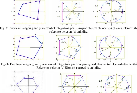
The element stiffness matrix in eq. (6) must be evaluated by integrating the integrand over the polygonal element domain. As it can be seen from eq. (9) that since the shape functions are rational polynomials in nature, the integrand in eq. (6) is also a rational polynomial. To integrate this rational polynomial over n-sided-polygon there are some scheme available in reference [3] and [4] but they have their own limitation. In the present study we employ two new schemes to obtain the optimal integration points, which involve two-level mapping of the physical polygonal elements. In the first level of mapping the field variables are transformed from the real space to a regular polygon using isoparametric mapping. In the second step, these transformed variables are then further transformed from regular polygon to the unit disc using Schwarz-Christoffel mapping. Schematic representations of this two-level mapping for quadrilateral element, pentagonal element and hexagonal elements are shown in figures (3), (4) and (5), respectively. In the proposed method, Schwarz-Christoffel (SC) mapping is done using SCPACK [6] subroutines in FORTRAN and MATLAB SC Toolbox [7] in MATLAB.

Fig. 3: Two-level mapping and placement of integration points in quadrilateral element (a) physical element (b) reference polygon (c) unit disc.

Fig. 4: Two-level mapping and placement of integration points in pentagonal element (a) Physical element (b) Reference polygon (c) Element mapped to unit disc.

Determination of Optimal Integration Points

As discussed earlier, first we map the physical polygon with any shape to a regular polygon using isoparametric mapping and then from the regular polygon to the unit disk using SC mapping. Integration points are defined on unit disk. For the present case of two-level mapping, the following approximation is used to integrate

( , )

f x y on an element in physical space:

1 1

( , )

( , )

( , )

(

,

)

r d

r

ip ip sc

n n

j i j i ip sc ij

i j

f x y dxdy

f

J d d

f

J J d d

f r Cos

r Sin

J J A

θ

ξ η

ξ η

ξ η

ξ η

θ

θ

Ω Ω Ω

= =

=

=

∫

∫

∫

∑∑

(11)

where (

r

_j,

θ

_i) is the coordinate of the integration point.

A

_ij are the weights associated with the integration points.

ip

J

and

J

_scare the Jacobian associated with isoparametric mapping and SC mapping, respectively.

Optimal Integration Points Based on Scheme 1

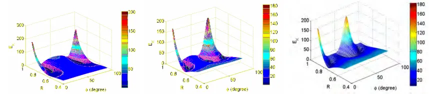
In scheme 1 we first calculate the stiffness matrix of the reference element using a known method with very good accuracy, although this is computationally very expensive. We call this the reference solution. Now we place the integration points on unit disk as shown in figs. (3-c), (4-c) and (5-c). Stiffness matrix is calculated based on these integration points. Stiffness matrix thus obtained is compared with the reference solution. The error in the stiffness matrix in terms of Frobenious norm error is calculated. The Frobenious norm of a matrix

K

is given by

2 1 1

K

n m

ij F

i j

k

= =

=

∑∑

(12)

The error in the stiffness matrix is defined as

100%

h F

k

h F

K

K

E

K

−

=

×

(13)

where

K

and

K

_h are the stiffness matrices obtained from reference solution and the proposed solution method (scheme 1) respectively. Now the values of (

r

,

θ

) are varied and error as defined in eq. (13) is plotted over the entire domain. The value of (

r

,

θ

) corresponding to the minimum error in

E

_k gives the coordinate of the optimal integration point.

Fig. 2: Error in Frobenius norm vs. coordinates

( , )

R

θ

of integration points on unit circle for (a) 4-node quadrilateral element (b) 5-node pentagonal element (c) 6-node hexagonal element.

Table 1: Optimal coordinate of integration points obtained based on scheme-1.

Quadrilateral Pentagonal Hexagonal

Optimum

R

0.749 0.7607 0.787

Optimum

θ

16.28 57.84 46.74

Optimal Integration Points Based on Scheme 2

h h

u u

E

u

∞ ∞

∞

−

=

(14)

Now from eq. (5) one has

1 1

and

_{h h}

u

=

K

−

f

u

=

K

−

f

(15) By substituting eq. (15) in eq. (14) we get

(

1 1

)

1 1

1 1

1 1

n

ij hij

h j

h

n ij j

K

K

K

K

u u

E

u

K

K

− − − −

=

∞ ∞

∞ −

−

∞ _∞

=

−

−

−

=

=

=

∑

∑

(16)

where

K

_and

K

_h are the stiffness matrices obtained from reference solution and the proposed solution method (scheme 2), respectively. Now the values of (

r

,

θ

) are varied and the error as defined in eq. (16) is plotted over the entire domain. The value of (

r

,

θ

) corresponding to the minimum error in

E

_∞ gives the optimal integration points.

Fig. 3: Error in Infinity norm of displacement vs. coordinates

( , )

R

θ

of integration points on unit circle for (a) 4-node quadrilateral element (b) 5-4-node pentagonal element (c) 6-4-node hexagonal element.

Table 2: Optimal coordinate of integration points based on scheme-2.

Quadrilateral Pentagonal Hexagonal

Optimum

R

0.749 0.761 0.797

Optimum

θ

16.28 57.84 45.68

As we can see from table-1 and table-2 that the optimal integration points for two different schemes are almost same and for quadrilateral mesh they are exactly same. In the rest of this paper we will use only one set of integration points (scheme-1) for all the numerical simulation.

VALIDATION OF SCHEME FOR POLYCRYSTALLINE MATERIAL

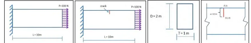
We will use a cantilever beam with axial load to study the performance of our integration scheme. Figure(4) shows the geometric and boundary configuration of the beam with crack and without crack.

For time being we will consider the polygonal element as polycrystal. We will render the crystallographic orientation for each element. Figure(5) shows few example of random crystaligraphic orientation distribution with respective standard deviation.

Fig. 5: Sample of random distribution of crystallographic orientation (a) with standard deviation 5.33, (b) with standard deviation 25.5, (c) with standard deviation 45.39.

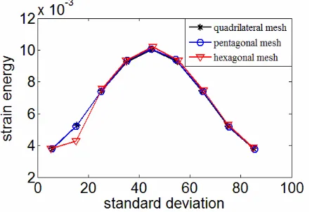
Let us now consider a microstructure based on regular hexagonal elements, where each grain is modeled by one hexagonal element. We first assume a distribution of the crystallographic orientation or material axis orientation based on the assumption that the total energy to form such microstructure during solidification would be minimum. In order to determine the distribution of the crystallographic orientations, we minimize the total strain energy. Figure 6 shows the variation of strain energy for various different distributions of crystallographic orientation. It is clear from the figure that among all those various crystallographic orientation distributions, the distribution which has least standard deviation of the random distribution about zero degree or ninety degree stores the minimum strain energy.

Fig. 6: Variation of strain energy for various different crystallographic orientation distributions.

Fig. 7: Discretization of quadrilateral grain structure explicitly meshed using commercial FEM package and solved (a) without crack (b) with crack.

Fig. 8: Discretization of pentagonal grain structure meshed explicitly using commercial FEM packages and solved (a) without crack (b) with crack.

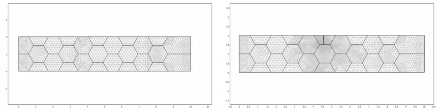
Fig. 9: Discretization of hexagonal grain structure meshed explicitly using commercial FEM packages and solved (a) without crack (b) with crack.

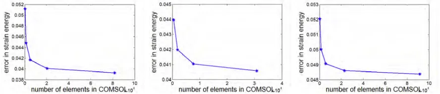
Fig. 10: Difference in strain energy without any crack obtained using the new polygonal element scheme and explicit FE mesh for (a) Quadrilateral grain structure (b) Pentagonal grain structure and (c) Hexagonal grain

structure.

CONCLUSION

A new polygonal finite element scheme has been proposed for numerical integration of rational polynomial in polygonal domain and the relative benefit of the new scheme to predict the deformation behaviour of polycrystalline material has been demonstrated. The main advantages here is that the polygonal elements representing each grain of the polycrystalline microstructure does not require explicit discretization of the grains as otherwise required in standard finite element. This can enable substantial speed-up in computation as well as allow efficient implementation of several physics based mechanisms in microstructure such as grain boundary sliding, dislocation migration and fundamental predictions about damage initiation. Importantly for crack related problem this scheme has been verified using XFEM framework, in which one does not need to discretize each polygonal grain and also due to the use of special enrichment function under XFEM framework one does not need any remeshing by conforming the shape of the crack. In our future work the crack propagation in polycrystalline types of material within XFEM framework will be considered.

Fig. 11: Difference in strain energy with crack obtained using the new polygonal element scheme and explicit FE mesh for (a) Quadrilateral grain structure, (b) Pentagonal grain structure and (c) Hexagonal grain structure.

REFERENCES

1. Wachspress EL. A rational basis for function approximation. Lecture notes in Mathematics, 228. Academic Press, Inc. New York: 1971.

2. Meyer M, Lee H, Barr AH. Generalized barycentric coordinates for irregular n-gons. Journal of Graphics Tools 2002; 7(1):13–22.

3. Sundararajan natarajan, St`ephane Bordas and D Roy. Mahapatra. Numerical integration over arbitrary polygonal domain based on Schwarz-Christoffel conformal mapping. Int. J. Numer.Meth. Engng., Vol. 80, 103–134 , 2009.

4. S.E. Mousavi, H. Xiao and N. Sukumar Generalized Gaussian Quadrature Rules on Arbitrary Polygons Int. J. Numer.Meth. Engng 2010; 81:660–670.

5. Belytschko T, Black T. Elastic crack growth in finite elements with minimal remeshing. International Journal for Numerical Methods in Engineering 1999; 45:601–620.

6. Trefethen LN, Numerical computation of the schwarz-christoffel transformation. SIAM Journal of Scientific and Statistical Computing 1980; 1:82–102.