ABSTRACT
ANYAH, RICHARD. Modeling the Variability of the Climate System over Lake Victoria Basin (Under the direction of Dr. Fredrick H.M. Semazzi)
The physical mechanisms associated with the diurnal to inter-annual variability of Lake Victoria Basin and regional climate are examined based on a three-tier modeling approach. First, diagnosis of eastern and the Horn of Africa climate variability, in which the Lake basin climate is intimately embedded, is performed based on two GCM ensemble simulations. The goal was to identify some of the systematic errors inherent in the GCMs before downscaling their output using regional climate model. The second part evaluates the downscaling ability of RegCM3 over eastern Africa based on multi-year ensemble simulations of the short rains season. Finally, the physical mechanisms associated with Lake Victoria Basin climate variability are investigated using a fully coupled RegCM3-3D lake modeling system.
A dissertation submitted to the Graduate Faculty of North Carolina State University
In partial fulfillment of the Requirements for the Degree of
DEDICATION
BIOGRAPHY
Richard ANYAH was born in Kisumu District in western Kenya. He attended Onjiko and Cardinal Otunga High Schools between 1980 and 1986 for his Secondary and High School education, respectively. After high school he joined Siriba Teachers College in 1987 where he graduated with a Diploma in Education in 1989, majoring in Mathematics. After a five year stint in teaching Mathematics at various High Schools in Kenya, he joined the University of Nairobi in 1993 for a Bachelor of Science Degree in Meteorology and graduated in 1997 with a BS(first class honors). Soon after finishing his undergraduate studies, he was awarded the University of Nairobi Merit Scholarship to pursue a Master of Science (MS) degree in Meteorology in October 1998.
ACKNOWLEDGEMENTS
I wish to recognize, with profound appreciation, the invaluable academic mentoring I received from my advisor, Professor Fredrick Semazzi. His humble demeanor and astute approach to scientific questions/discussions made working with him not only fulfilling academically, but also immensely enriched my personality. My sincere thanks are also due to all my advisory committee members; Dr. Lian Xie, Dr. Adel Hanna and Dr. Dev Niyogi for their guidance throughout the course of my research. I am also greatly indebted to Prof. Laban Ogallo who helped to mould my unstructured thoughts of venturing into regional climate modeling into a reality. Dr. Joseph Mukabana also inspired me with his teaching of Dynamic Meteorology at the University of Nairobi.
The National Science Foundation (NSF), through a number of grants awarded to my academic advisor during the course of my study, primarily funded my research. The numerical model experiments were performed at North Carolina State University’s High Performance Computing Center and on the National Center for Atmospheric Research (NCAR) supper computers. NCAR is sponsored by NSF.
TABLE OF CONTENTS
Page
LIST OF TABLES... x
LIST OF FIGURES ... xi
CHAPTER 1 1 INTRODUCTION... 1
1.1 General climatology and seasonal to inter-annual variability of East Africa ... 7
1.2 Location and Physical dimensions of Lake Victoria ... 10
1.3 Hydrology and drainage of Lake Victoria basin... 10
1.4 Climatology of Lake Victoria Basin... 11
1.5 The study Objectives... 13
1.6 Statement of the research problem and Justification of the study ... 15
1.7 Related previous climate modeling studies... 16
1.8 Thesis Outline ... 21
CHAPTER 2 2 DESCRIPTION OF NUMERICAL MODELS AND VALIDATION DATA... 24
2.1 Description of component models of the RegCM3-POM system ... 24
2.1.1 RegCM3 Model ... 24
2.1.2 Princeton Ocean Model (POM) ... 26
2.1.3 Coupling of RegCM3 and POM via surface fluxes ... 27
2.1.4 Initial and boundary conditions for RegCM3 ... 30
2.2 Model Validation Data... 34
2.2.1 Rain gauge observed rainfall data... 35
2.2.2 Climate Prediction Center Merged Analysis of Precipitation Data (CMAP)..35
2.2.3 Climate Research Unit (CRU TS 2.0) Dataset... 36
2.2.4 Tropical Rainfall Measuring Mission (TRMM)/Microwave Imagery(TMI) Data ………..36
CHAPTER 3 3 VARIABILITY OF THE GREATER HORN OF AFRICA CLIMATE BASED ON GCM ENSEMBLE SIMULATIONS... 38
3.1 Introduction... 39
3.2 Data and methods of analysis ... 43
3.2.1 Observed rainfall and wind data ... 43
3.2.2 NCAR-CAM2.0.1 model ensemble... 44
3.2.3 NASA-CCM3 ensemble ... 45
3.3 Empirical Orthogonal Functions (EOF) technique ... 46
3.4 Results and discussions... 47
3.4.1 GCM ensemble and observed rainfall climatology ... 47
3.4.2 Latitude-time evolution of rainfall during the short rains season ... 50
3.4.3 Relationship between 925hPa circulation pattern and tropical Oceans SST anomalies during 1961 and 1997 wet events ... 64
3.4.4 Circulation and specific humidity (moisture) anomaly relationships during 1961 and 1997 wet episodes ... 69
3.4.5 EOF analysis of monthly mean rainfall over the GHA domain... 73
3.4.7 Uncertainty in NCAR-AGCM ensemble simulations of GHA rainfall
variability ... 92
3.4.8 Trends in rainfall variability over GHA... 94
3.4.9 Trends in the mean surface temperatures over Eastern Africa ... 98
3.5 Conclusions... 102
CHAPTER 4 4 VARIABILITY OF EAST AFRICA CLIMATE BASED ON MULTI-YEAR RegCM3 SIMULATIONS... 106
4.1 Introduction... 106
4.2 Model simulations and Validation Data ... 111
4.2.1 Model simulations... 111
4.2.2 Validation data ... 111
4.3 Results and discussions... 112
4.3.1 Simulated versus observed monthly rainfall climatology... 112
4.3.2 Latitude-time evolution of rainfall over East Africa... 120
4.3.3 Rainfall climatology over homogeneous climate sub-regions... 124
4.3.4 Inter-annual variability of rainfall over homogeneous climate zones ... 127
4.3.5 EOF analysis of simulated and observed monthly rainfall ... 137
4.3.6 RegCM3, NCEP and NASA-CCM3 mean circulation patterns at 850hPa .. 152
4.3.7 Comparison between simulated and observed seasonal mean surface temperature ... 157
CHAPTER 5
5 HYDRODYNAMIC CHARACTERISTICS OF LAKE VICTORIA BASED ON
IDEALIZED 3D LAKE MODEL SIMULATIONS... 165
5.1 Introduction... 166
5.2 Formulation of the elliptic bathymetry/geometry for Lake Victoria ... 172
5.3 Results and Discussions... 173
5.3.1 Lake surface temperature evolution... 173
5.3.2 Horizontal cross sections of the temperature profile ... 181
5.3.3 Lake currents... 186
5.3.4 Surface temperature distribution... 194
CHAPTER 6 6 PHYSICAL MECHANISM ASSOCIATED WITH THE COUPLED VARIABILITY OF LAKE VICTORIA BASIN CLIMATE... 199
6.1 Introduction... 200
6.2 Results and Discussions... 203
6.2.1 Simulated versus satellite estimated (TRMM) monthly mean rainfall over the lake 203 6.2.2 Comparison between RegCM3-POM and RegCM3-1D simulations... 210
6.2.3 Diurnal variability of Lake Victoria Basin climate based on coupled model simulations ... 213
6.2.4 Diurnal cycle and daily rainfall variability over Lake Victoria... 223
6.2.5 Daily rainfall variability over Lake Victoria ... 227
6.2.6 Contribution of large scale moisture to the Lake Basin rainfall variability.. 232
6.2.9 Effects of land surface/use changes on basin-wide rainfall climate variability 254
6.2.10 Rainfall variability as a response of lower boundary forcing ... 258
6.3 Conclusions... 263
CHAPTER 7 7 SUMMARY, CONCLUSIONS AND RECOMMENDATIONS... 267
7.1 Summary ... 267
7.2 Conclusions... 269
7.3 Recommendations... 277
LIST OF TABLES
Table 4.1: Number of times RegCM3 model simulates the same/not same rainfall anomaly compared to observations(CRU) over four homogeneous climate sub-regions in October ... 131 Table 4.2: Same as table 4.1, but December... 133 Table 4.3: Same as Table 4.2, but for OND... 135 Table 4.4: The total rainfall variance(5) explained by three leading eigenmodes derived from RegCM3 simulated rainfall and observations(CRU)... 138 Table 4.5: Correlations coefficients among RegCM3 and CRU three leading EOF temporal
patterns... 139 Table 6.1: Summary of Numerical Experiments ... 232 Table 6.2: Percent differences between large scale moisture anomaly experiments and CTRL ... 233 Table 6.3: Numerical experiments to investigate sensitivity of Lake Basin climate to land
LIST OF FIGURES
Figure 1.1: Long-term mean annual rainfall total over Lake Victoria Basin based (adapted
from Asnani, 1993) ... 13
Figure 1.2: Conceptual modeling framework for the climate variability of Lake Victoria Basin and contiguous regions ... 23
Figure 2.1: Topographical features of the outer domain, with areas higher than 1000m shaded ... 34
Figure 3.1: 30-year (1961-1990) rainfall climatology. (a) NCAR-CAM2.0.1 (b) NASA-CCM3 (c) CRU (d) Wilmont ... 49
Figure 3.2: Latitude-time evolution of rainfall in mm/day over GHA ... 52
Figure 3.3: The north-south rainfall (mm/day) evolution over the GHA during the flood events in 1961 and 1997 ... 55
Figure 3.4: Differences between rainfall amounts/patterns during November 1961 and 1997 wet events... 56
Figure 3.5: Mean 925hPa circulation pattern in October... 59
Figure 3.6: Mean 925hPa circulation pattern in November... 60
Figure 3.7: Mean 925hPa circulation pattern in December. ... 61
Figure 3.8: Mean and anomaly circulations at 850hPa in November 1961 (a) CAM2.0.1 ensemble mean circulation (b) NCEP reanalysis mean circulation (c) CAM2.0.1 1961 circulation anomaly (d) NCEP 1961 circulation anomaly... 62
Figure 3.9: Same as figure 3.8, but for the 1997 wet episode... 63
Figure 3.10: Circulation and SST anomaly fields in November 1961. (a) CAM2.0.1 ensemble average(b) NCEP reanalysis. Regions of positive SST anomalies are shaded ... 67
Figure 3.11: Circulation and SST anomaly fields in November 1997. (a) GCM ensemble average (b) NCEP reanalysis. Regions of positive SST anomalies are shaded ... 68
Figure 3.13: Same as figure 3.12, but for November, 1997... 72
Figure 3.14: Spatial patterns of CAM2.0.1 ensemble average and CMAP EOF1(1979-2000). Upper panels(OCT). Lower panels(November) ... 76
Figure 3.15: Same as figure 3.14, but for December and OND... 77
Figure 3.16: Comparison between CAM2.0.1 and CMAP EOF1 temporal patterns derived from the 22-year(1979-2000) analysis... 78
Figure 3.17: Spatial patterns of GCM ensemble average and CMAP EOF2 (1979-2000). Upper panels (October). Lower panels (November)... 80
Figure 3.18: 22-year time series of EOF2... 81
Figure 3.19: CAM2.0.1and CMAP EOF2 spatial patterns (1979-2000). Upper panels (December). Lower panels (OND) ... 82
Figure 3.20: Same as figure 2.18, but for December and seasonal mean ... 83
Figure 3.21: Comparison between CAM2.01 and CCM3 EOF1 spatial patterns in October(1961-1990)... 85
Figure 3.22: Comparison between CAM2.0.1 and CCM3 EOF1 temporal patterns... 85
Figure 3.23: Same as figure 3.21, but for December ... 87
Figure 3.24: Same as figure 3.22, but for December ... 87
Figure 3.25: Same as figure 3.21, but for OND... 89
Figure 3.26: Same as figure 3.22, but for OND... 89
Figure 3.27: Comparison between CAM2.0.1 and CCM3 EOF2 spatial patterns for seasonal mean rainfall(1961-1990) ... 91
Figure 3.28: Comparison between CAM2.0.1 and CCM3 EOF2 temporal patterns... 91
Figure 3.29: EOF1 time series for selected members of CAM2.0.1 ensemble ... 93
Figure 3.31: 5-point running mean of the EOF2 time series of CAM2.0.1 ensemble average, CMAP and gauge observations over East Africa ... 97 Figure 3.32: Comparison of normalized monthly mean surface temperature between CRU
and GCM ensemble average ... 100 Figure 3.33: Comparison of normalized monthly mean surface temperature between CRU
and GCM ensemble average ... 101 Figure 4.1: The monthly rainfall climatology for October. (a) RegCM3 forced by GCM
output (b) RegCM3 forced by NCEP reanalysis (c) Observations (0.5ox0.5o CRU
gridded data: bottom panel) ... 115 Figure 4.3: The monthly rainfall climatology for December. (a) RegCM3 forced by GCM
output (b) RegCM3 forced by NCEP reanalysis (c) Observations (0.5ox0.5o CRU gridded data... 117 Figure 4.4: Monthly long term mean simulated rainfall difference between RegCM3 forced
by GCM and NCEP reanalysis ... 119 Figure 4.5: Latitude-time evolution of rainfall(mm/day) over East Africa during short rains
season, 1988. (a) RegCM3 coupled to 1D-Lake model (b) same as a, but without lake model (c) CRU data (d) CMAP ... 123 Figure 4.6: Comparisons of simulated and observed rainfall climatologies over different
homogeneous climate sub-regions... 126 Figure 4.7: Seasonal mean rainfall total over different homogeneous climate sub-regions. 127 Figure 4.8: Simulated versus observed inter-annual variability over different homogeneous
climate sub-regions in October ... 130 Figure 4.9: Same as figure 4.8, but for December ... 132 Figure 4.10: Same as figure 4.8, but for OND... 134 Figure 4.11: Comparisons between RegCM3 simulations and observed spatial averaged
seasonal mean rainfall variability over four homogeneous sub-regions over East Africa ... 136 Figure 4.12: Spatial and temporal patterns of EOF1 in October. (a) spatial pattern of
Figure 4.14: Same as figure 4.12, but for December ... 144
Figure 4.15: Same as figure 4.12, but for seasonal mean rainfall (OND). ... 145
Figure 4.16: Spatial and temporal patterns of EOF2 in October (a) spatial pattern of RegCM3 (b) spatial pattern of CRU (c) temporal patterns ... 148
Figure 4.17: Same as figure 4.16, but for November... 149
Figure 4.18: Same as figure 4.16, but for December ... 150
Figure 4.19: Same as figure 4.16, but for OND... 151
Figure 4.20: Mean circulation pattern over the larger(African) Domain (a) RegCM3-NCEP(b) RegCM3-GCM (c)NCEP reanalysis (d) CCM3 ... 154
Figure 4.21: Same as figure 4.20, but fort November ... 155
Figure 4.22: Same as figure 4.20, but for December ... 156
Figure 4.23: Inter-annual variability of mean surface temperature over East Africa ... 158
Figure 4.24: Mean surface temperature fluctuations over homogeneous climate sub-regions in October (a) NEK (b) CKE (c) CST (d) CTZ ... 160
Figure 5.1: Idealized versus real geometry/bathymetry of Lake Victoria ... 173
Figure 5.2: Initial temperature profile... 174
Figure 5.3: Vertical temperature profiles after (a) 5 days (b) 10 days (c) 1 month (d) ... 177
Figure 5.4: Temperature evolution at the surface ... 179
Figure 5.5: Same as figure 5.4, but at 40m depth ... 180
Figure 5.6: Cross section of the temperature profiles after 2, 15 and 30 days of model integration ... 183
Figure 5.7: Similar to figure 5.6, but for 45 and 60 day comparisons... 184
Figure 5.8: Cross section of the vertical profile of water current after 2 days (upper panels), 15 days(middle panels) and 30 days(bottom panels)... 185
Figure 5.10: Same as figure 5.9 but after 30 days (upper panels) and 60 days (lower panels) ... 190 Figure 5.11: Similar to figure 5.9, except the area of the lake is relatively larger... 191 Figure 5.12: Similar to figure 5.10, but after 30 and 60 days of model integration ... 192 Figure 5.13: 30-day simulated mean current with idealized surface stress forcing, but using
20km resolution bathymetry data for Lake Victoria... 193 Figure 5.14: Surface temperature distribution after 5 days (upper panels)... 196 Figure 5.15: Same as figure 5.14, after 30 days(upper panels) and after 60 days (lower
panels)... 197 Figure 5.16: Simulated surface temperature with uniform wind stress forcing, but real
bathymetry (a) after 5 days (b) after 15 days (c) after 30days... 198 Figure 6.1: Comparison between RegCM3-POM simulated monthly mean rainfall and.... 206 Figure 6.2: Same as figure 6.1, but for November, 2000... 207 Figure 6.3: Same as figure 6.1, but for November, 2002... 208 Figure 6.4: Over-lake averaged rainfall (a) northern half (b) southern half (c) over-lake
anomaly based on 1998-2002 average... 209 Figure 6.5: Differences between RegCM3-POM and RegCM3-1D rainfall simulations for
November. (a) 1998 (b) 2000 (c) 2002 ... 212 Figure 6.6: Mean circulation pattern at 850hPa over the Lake Basin at 3LST (a) RegCM3-1D (b) RegCM3-3D (c) Difference ... 217 Figure 6.7: Same as figure 6.6, but at 15LST ... 218 Figure 6.8: Overlay of 850hPa mean flow on convective precipitation field at 3LST over the Lake Basin (a) RegCM3-1D (b) RegCM3-POM... 219 Figure 6.9: Same as figure 6.8, but for 15LST ... 220 Figure 6.10: Same as figure 6.8, but the mean flow is overlaid onto non-convective
Figure 6.12: 3-hourly total rainfall over four different quadrants over the Lake ... 225
Figure 6.13: Same as figure 6.12, but for November 2000... 226
Figure 6.14: Same as figure 6.12, but for November 2002... 227
Figure 6.15: Simulated and TRMM mean daily rainfall averaged ... 230
Figure 6.16: Same as figure 6.15, but for rainfall averaged ... 231
Figure 6.17: Simulated rainfall (mm) over Lake Victoria basin with large moisture through eastern boundary reduced by (a) 20% (b) 50% (c) 80%... 236
Figure 6.18: Simulated rainfall over the Lake Basin with large scale moisture across different boundaries reduced by 50% (a) Control (b) northern boundary (c) southern boundary (d) western boundary (e) eastern boundary ... 237
Figure 6.19: Comparisons between simulations with large scale moisture reduced by 50% (a) (a) Left panels (all the four boundaries) (b) right panels (only eastern boundary)... 238
Figure 6.20: Different types of topographical heights used to investigate the response of Lake Basin climate to topographic-induced circulations... 241
Figure 6.21: Vertical velocity profiles in the TPALL experiments (a) 3LST (b) 15LST... 245
Figure 6.22: Profiles of vertical velocity differences between TPALL and CTRL experiments (a) 3LST (b) 15LST... 246
Figure 6.23: Difference between convergence/divergence fields at 925hPa (a) 3LST (b) 15LST. Positive values show regions of net divergence, and negative values show regions of net convergence (values x 10-4m2s-2) ... 247
Figure 6.24: Same as figure 6.22, but for TPEA case... 251
Figure 6.25: Same as figure 6.24, but for TPEA-CTRL case ... 252
Figure 6.26: Same as figure 6.22, but for TPEA-CTRL case ... 253
Figure 6.27: Vertical velocity profiles in the LBOG experiment ... 256
Figure 6.28: Profiles of LBOG-CTRL vertical velocity differences ... 257
CHAPTER 1
1 INTRODUCTION
The geography and physical characteristics of East Africa presents a classic setting where complex terrain and land surface heterogeneities exert significant influence on the regional climate. The high mountains, large inland lakes, fast growing urban centers and variable vegetation cover/types modulates regional climates through the generation of orographic precipitation, lake/land breeze circulation and urban heat island (Leung et al., 2003). The East Africa Great Rift Valley system that hosts several of the largest and deepest tropical lakes such as Lake Victoria (the largest tropical fresh water lake), Lake Tanganyika (the deepest tropical lake) and Lake Malawi also forms a unique, but enabling environment for interactions between local and large scale circulations. These features and their consequent interactions with large-scale climate forcing mechanisms contribute significantly to the diverse spatial patterns of climate (rainfall) over East Africa that also changes within very short distances (Nicholson, 1996; Ininda, 1998).
However, the ITCZ which crosses the region twice a year; March through May (long rains season) and October through December (short rains season) is mainly responsible for the climatological and the predominantly bimodal rainfall pattern over the region. The onset of seasonal rains has been shown to lag the ITCZ position by three-to-four weeks (Okoola, 1998). An extended discussion of the general climatology of East Africa is provided in a later section.
A comprehensive study of tropical circulation dynamics generally requires an in-depth investigation of interactions of cumulus convection and meso-scale circulations with large scale motions (Holton, 2004). Equatorial eastern Africa is one such region where complex interactions among an array of environmental and geographic variables with the prevailing circulation takes place on sub-seasonal to inter-annual scales. However, better understanding of such interactions demands an integrated, process-based approach. Hence, in this study dynamical downscaling technique based on a regional climate model (RCM) coupled to a three dimensional Lake model is employed to investigate some of the dominant physical and dynamical mechanisms responsible for Lake Victoria Basin and regional climate variability.
techniques often do not provide enough scope to unravel the cause-effect mechanisms responsible for regional climate variability because of their primary dependence on sparse observations.
In general, both the GCM and “conventional” observational/empirical analysis techniques cannot provide sufficient climate information needed for seasonal predictions as well as regional climate change projections. Furthermore, whereas the foundation and success of predictability of large-scale seasonal climate is based mainly upon the interactions of the atmosphere with the slow-varying surface boundary conditions (e.g sea surface temperatures (SSTs) and soil moisture), predictability of regional scale seasonal climate depends upon the interactions between the anomalies of atmospheric circulation and geographic features such as terrain, land cover, and oceans or lakes (Goddard et al., 2001, Leung et al., 2003).
systematically examine the variability and sensitivity of different climate variables to different forcings (Wang et al., 2004). In other words, RCMs provide sufficient scope for investigating multi-processes that may combine to influence regional climate variability. Besides, when coupled to appropriate land surface, hydrologic or lake models the enhanced resolutions of RCMs permits adequate representation of land surface-atmosphere interactions which improves the simulations of detailed precipitation, temperature and surface hydrological features (Small et al., 1999).
The present study primarily focuses on Lake Victoria basin and the regional climate in which the lake’s climate is also intimately embedded. Principally, the emphasis is to improve understanding of the various physical processes that influence the diurnal, sub-seasonal, seasonal and inter-annual variability of Lake Victoria Basin and regional climate. The effects of the interactions among regional orography, Lake Victoria, land cover/use changes and large scale forcing are studied using a three dimensional lake model coupled to a regional atmospheric climate model.
The intimate relationship between Lake Victoria basin and regional climate on seasonal to inter-annual scale has also been well demonstrated in a number of previous studies (e.g Stager et al., 1986; Anyamba, 1983; Nicholson and Kim, 1998; Phillipon et al., 2002; Lehman, 1998 and Anyah and Semazzi, 2004). Nicholson (1996) used a long time series of historical observations, dating back to the late 1880s and derived from both historical reconstructions and modern instruments and showed that historical changes in the levels of Lake Victoria and other East Africa Rift Valley lakes have been fluctuating concomitantly with the regional climatic conditions. For, example, the above average rainfall experienced over the region during 1961/62 floods led to a record lake level rise of over 2m (Anyamba, 1984). In contrast, during the early periods of the 19th century when the region experienced frequent droughts, the lake level also fell significantly (Nicholson, 1997; Lehman, 1997). This further indicates that the climate of the Lake (Basin) is intimately coupled to the regional climate.
importance of the basin. This economic potential translates to direct support for more than one third (more than 30 million) of the population of the riparian communities. In recognition of this economic potential, the riparian countries of Kenya, Uganda and Tanzania under the aegis of East Africa Community Development Agenda strategy have designated the Lake Basin as a regional economic growth zone (LEVMP, 2003). However, the major socio-economic activities within Lake Basin are highly sensitive to climate perturbations. Climate variations are especially linked to the lake conditions through mechanisms of heat budget and mixing regimes that are consequences of atmosphere-lake interactions (Lehman, 1998). This means that integrating the role of the lake into regional climate variability studies is a critical ingredient in the formulation and sustainability of the regional economic policies.
Hence, an integrated study of the climate variability, predictability and changes over the Lake Basin has potential beneficial input into regional economic development agenda. However, in order to accomplish such a study, it is important to start by investigating how some of the current research tools capture the regional climate variability associated with large scale atmospheric circulation systems. Therefore, the strategy adopted in this study was to first undertake comprehensive diagnoses of eastern Africa climate variability based on GCM ensemble simulations before using a regional climate model (RegCM3) and a fully coupled RegCM3-Lake model for dynamical downscaling of the GCM output over the Lake Victoria Basin. In this case the deficiencies of the large scale driving fields that may undermine optimal performance of the regional model over the Lake Basin are identified.
The evaluation of the GCM performance is primarily based on the ability of the model to reproduce the mean climate and the inter-annual variability over eastern and the Horn of Africa (GHA) sub-region. Brief descriptions of the observed climatology and some of the peculiar climatic and physiographic aspects of East Africa and Lake Victoria Basin are given in the following sub-sections.
1.1 General climatology and seasonal to inter-annual variability of East Africa
rainfall pattern experienced over many parts during March to May (long rains) and October to December (short rains).
Thus the climatological rainfall pattern over the region is intimately linked to the north-south movement and near surface location of the ITCZ, which itself follows the inter-hemispheric migration of the overhead sun. The northeast (NE) and southeast (SE) monsoons normally trails the ITCZ and the two main rainfall seasons are experienced during the transition periods between the peaks of the monsoons. However, over southern Tanzania unimodal climate regime dominates, with the only main rainfall season occurring during boreal winter (December through February). Also some parts of western Kenya, western and northwestern Uganda are characterized by trimodal regimes since they often receive significant amounts of rainfall during July through September. Rainfall during this period is mostly associated with the penetration of the mid-tropospheric moist westerly flow from the Atlantic Ocean and the tropical rainforest (Congo) air mass (Davies et al., 1985; Mutai el al.,1998; Anyamba, 1984). However, superimposed on these prevailing synoptic systems are the local circulations generated by the complex orography, large inland lakes and the Indian Ocean leading to substantial amount of rainfall throughout the year near the large water bodies and over the highlands.
2000; Bowden et al., 2004). In particular, El Niño/Southern Oscillation (ENSO) anomaly patterns are closely linked to the anomalous dry and wet seasons. The warm phase of ENSO (El Niño) is associated with excess rainfall and flooding, while the cold phase (La Niña) often coincides with extreme drought conditions (Ogallo, 1988; Nicholson, 1996).
Indeje et al. (2000) and Mutai et al. (2000) have summarized the dominant sources of inter-annual variability over eastern Africa to include: -
(a) El Niño/Southern Oscillation(ENSO)
(b) Indian Ocean Zonal temperature gradient (or Dipole Mode) (c) Tropical Atlantic Ocean temperature anomalies
(d) Quasi-biennial oscillation (QBO) in the equatorial zonal wind (e) Orographic forcing
In addition to the above, Shreck and Semazzi(2004) recently showed that there is a strong Global Warming footprint on the regional climate variability, especially during the past two decades.
1.2 Location and Physical dimensions of Lake Victoria
The approximately rectangular (saucer)-shaped Lake Victoria (Ochumba, 1996) is located in the middle of the three East African states, with most of its northern half in Uganda, southern half in Tanzania and a relatively small northeastern portion gulfing into Kenya. The lake is located within 0.2oN-3.0oS and 31.5oE-34.5oE and is about 400km long and 280km wide. Its extensive water surface, estimated at 69,000km2 is situated at an elevation of about 1134m AMSL between the shoulders of western and eastern Rift Valley system. The lake’s drainage basin covers an area of about 195,000km2 that extends to parts of Rwanda and Burundi to the west of the lake. Compared to other Rift Valley lakes, Lake Victoria is quite shallow; with mean (maximum) depth of 40m(84m) and a coastline of about 3440km all round the lake perimeter (Ochumba, 1996). The water volume of the lake is only 2760km3 per annum (Coulter and Spigel, 1996), compared to Lake Tanganyika’s 18,880km3 and Lake Malawi’s 84,000km3. Comparison of the physiographic statistics of the large East Africa Great Rift Valley and some of the world largest lakes is presented in Table 1.
1.3 Hydrology and drainage of Lake Victoria basin
The hydrologic balance of the lake is dominated by rainfall and evaporation (Piper, 1986; Nicholson and Yin, 2000), with runoff contributing a negligible fraction. Thus the mean annual rainfall over the lake is in near perfect balance with evaporation (Nicholson and Yin, 1998; Ba and Nicholson, 2000). Sene and Plinston(1994) and Nicholson et al. (2000) have indicated that more than 90% of the annual water input into the Lake Basin is from precipitation onto the lake surface. This further demonstrates that precipitation and evaporation are the dominant terms in the water budget of the lake. However, due to inadequate meteorological measurements the lake’s water balance/budget cannot be conclusively evaluated.
1.4 Climatology of Lake Victoria Basin
The large-scale precipitation over the lake is mainly initiated from the easterly/southeasterly (Indian Ocean) monsoon flow that transports maritime moisture into the interior of East Africa. The humid Congo air mass has also been linked to significant rainfall amounts received over the western and northwestern parts of the lake (Asnani, 1993). However, convective precipitation over the Lake Basin is considered to come mainly from recycling of lake water via evaporation and re-precipitation on the lake surface (Nicholson, 1996; Nicholson and Kim, 1998). In terms of inter-annual variability, Lake Victoria Basin climate is characterized by periodic episodes of anomalously wet/dry conditions. Some of the most recent events include the 1961/62 and 1997/98 floods that left behind a huge trail of damage to property and infrastructure. The 1961/62 floods were associated with a strong zonal SST gradient over the equatorial Indian Ocean and mid-troposphere westerly flow from Tropical Atlantic (Anyamba, 1984; Anyah and Semazzi, 2005). On the other hand, the 1997/98 floods coincided with one of the warmest ENSO episodes (strongest El Niño) of the last century as well as very strong Indian Ocean dipole mode. Hence, the inter-annual variability of the Lake Basin is also closely linked to the SST anomalies over the global ocean basins.
intense insolation throughout the year. Lake water temperatures also usually follow the magnitude of solar radiation input but with some lag (Bugenyi and Magumba, 1996). Thus, based on sample measurements over a number of points over the lake surface, the mean monthly solar radiation is estimated at 240-270W/m2 and the surface water temperatures ranges between 24oC and 28oC(Ochumba, 1996; Bugenyi and Magumba, 1996).
Figure 1.1: Long-term mean annual rainfall total over Lake Victoria Basin based (adapted from Asnani, 1993)
1.5 The study Objectives
variability of Lake Victoria and regional climate. Since the primary vehicle employed to investigate these mechanisms is a coupled lake-atmosphere modeling system, some of the research questions this study addresses include,
(1) How skilful can the GCMs predict (nowcast) the large-scale features of the East Africa climate?
(2) How well do the RCMs reproduce and predict the detailed features of the regional climate when nested in the GCMs or driven by analysis of observations?
(3) Can RCMs, when fully coupled to 3D-lake models, improve understanding, characterization and prediction of mechanisms associated with the Lake Basin and regional climate variability on diurnal, sub-seasonal, seasonal and inter-annual scales?
Given the spatial scale of interest, the focus of this study is to address questions 2 and 3. Nevertheless, question 1 is also addressed in a fairly comprehensive detail since any biases in the GCMs would subsequently undermine the downscaled climate features using RCMs. In sum, the three primary objectives of this study are:-
Objective 1: Diagnose the intra-seasonal and inter-annual variability of eastern Africa climate based on two GCMs ensemble simulations (i.e 50-year NCAR-AGCM ensemble and a 30-year NCAR/NASA CCM3 ensemble)
Objective 2: Characterize East African climate variability based on regional climate model (RegCM3) ensemble simulations with lateral boundary forcing taken from analysis of observations (NCEP reanalysis) and GCM output.
orographic-induced circulations, lake-induced circulations, Lake geometry/bathymetry changes and land surface/land use changes within the lake catchment.
1.6 Statement of the research problem and Justification of the study
This study focuses on understanding the dominant physical mechanisms that affect sub-seasonal, seasonal and inter-annual variability of Lake Victoria Bain and the regional climate. Lake Victoria and its hinterland is one of the major economic hubs in East Africa. Besides having an agriculturally rich hinterland, the lake also supports and sustains important fisheries, hydroelectric power supply and is a potent source of both domestic and industrial water supply. According to World Bank Development Indicators (1998), the annual economic product of the lake basin is estimated at between 3 and 4 billion US dollars and directly supports more than one third (30 million) of the population of the riparian communities. However, many of the socio-economic activities within the Lake Basin are very sensitive to climate fluctuations (Nicholson and Kim, 1998).
climate. In particular, deforestation within the catchment areas due to population pressure may not only have a negative feedback on the hydrological balance and lake basin climate, but also threatens the very existence of the lake altogether.
The aforementioned factors illustrate a multi-pronged onslaught on the lake, its ecosystem and climate. Hence, to improve understanding of the variability and changes in the basin and regional climate this study emphasizes a process-based approach using a fully coupled 3D-Lake/atmospheric modeling system.
1.7 Related previous climate modeling studies
meteorological input to force the lake model in ‘stand-alone’ simulations also does not permit feedbacks between the lakes and the atmosphere. The approach proposed by Bonan(1995) in which the surface fluxes are calculated separately over land and water fractions within each grid-cell of a GCM may be more realistic, but still does not allow full three-dimensional interactions between the atmosphere and the large inland lakes. A few studies have employed a fully coupled three-dimensional lake/atmospheric modeling system to study the catchment-scale and regional climates around large inland lakes (Song et al., 2002, 2004).
land-lake(sea) breeze circulations over lake Victoria region and along the East Africa coast. Their study indicated that strong horizontal velocity convergence /divergence between large-scale and meso-scale circulations occurred over the highlands east of Lake Victoria (in agreement with Okeyo, 1982, 1987) and along the coast. However, whereas these studies highlighted the important contributions of the local forcing on the diurnal variability of the regional climate they were based on a simplified one-dimensional land-lake (sea) thermal contrast formulation that does not permit two-way lake-atmosphere interactions. Furthermore, the above studies were based on specific weather events and did investigate the potential effects of the lake on regional climate on sub-seasonal to inter-annual scales since their primary objective was numerical weather prediction. The present study examines some of the physical and dynamical mechanisms associated with both short term (weather) and long term (climate) variability over the Lake Basin and employs a fully coupled lake-atmosphere modeling system.
However, the major model deficiency evident from the simulations of Sun et al., (1999) was over estimation of rainfall throughout the domain. Also use of a simple 1D model for Lake Victoria could not allow two-way interactions between the lake and atmosphere in order to better characterize the contribution of the lake on regional climate variability and might have also contributed to over-estimation of rainfall over the lake. Besides, in the absence of multi-year simulations (ensemble) of the short rains season, no reliable model climatology and other useful statistics could be generated to comprehensively characterize and understand the sub-seasonal to inter-annual variability of the basin and regional climate.
results further demonstrated that a fully coupled system produced more realistic simulations of rainfall over and around Lake Victoria compared to cases where a simple one dimensional thermal diffusion equation was used to compute flux exchanges between the lake and ambient atmosphere.
In spite of the milestones achieved by Sun et al. (1999a, b) in the customization and initial application of RegCM2-1D over East Africa and Song et al., (2001) in demonstrating the improvements achieved by applying a fully coupled RegCM2-3D Lake system to simulate Lake Victoria Basin climate, still a number of limitations that undermined the optimal performance of the model system over East Africa/Lake Victoria Basin still existed. Some of these limitations included;-
(i) Lack of multi-year model ensemble simulations in order to generate appropriate model climatology as well as other statistics of sub-seasonal, seasonal and inter-annual variability that would help to comprehensively evaluate the capability of the model across different climate regimes.
(iii) Course spatial and temporal resolution of SSTs used for lower boundary forcing. Since the computational domain includes a large portion of the western Indian Ocean, the model’s ability to capture the correct evolution of SSTs over the Ocean is quite important.
Some of the aforementioned deficiencies and limitations been addressed in the present study by applying the latest version of the regional climate model (RegCM3) with improved radiation and sub-grid scale precipitation parameterization schemes. These are described detail later in Chapter 2.
1.8 Thesis Outline
COUPLED CLIMATE VARIABILITY OVER LAKE VICTORIA BASIN (MODELING FRAMEWORK)
Figure 1.2: Conceptual modeling framework for the climate variability of Lake Victoria Basin and contiguous regions
Modeling the variability of the climate
system over Lake Victoria Basin
Diagnostics (GCM Ensemble)
)
NCAR-CAM2
(~280kmx 280km) (~110kmx140km)NASA-CCM3
Mean Climate/variability
NCEP/ERA40
(~270kmx270km)
ICBC RegCM3
(60km)
RegCM3-POM(20km) (Coupled)
Lake Basin Climate Variability/sensitivity:
CHAPTER 2
2 DESCRIPTION OF NUMERICAL MODELS AND VALIDATION DATA
The two components of the regional atmospheric climate/lake modeling system as well the various model validation data sets are described in the next sections.
2.1 Description of component models of the RegCM3-POM system
2.1.1 RegCM3 Model
RegCM3 is a three-dimensional primitive equation atmospheric model (Giorgi et al., 2003). It is an improved and augmented version of the NCAR-RegCM2 (Giorgi et al., 1993 b,c). The model uses a terrain-following (sigma-pressure) vertical coordinate system and has up to 23 vertical levels with the model top at 50mb. The radiation physics calculations are based on the latest version of NCAR-CCM3 scheme (Kiehl et al., 1996). Although this scheme fundamentally resembles the CCM2 radiation physics package used in NCAR-RegCM2 it also includes a new component for computing the effects of additional greenhouse gases (NO2, CH4, and CFCs), aerosols and cloud ice. The land surface physics parameterizations are based on Biosphere-Atmosphere-Transfer Scheme (BATS1e: Dickinson et al., 1993) in which a standard surface drag coefficient based on surface-layer similarity theory is applied to calculate sensible, water vapor and momentum fluxes at the surface. The drag coefficient is based on the surface roughness and stability of the surface layer.
RegCM2 has been replaced with its simplified version that instead uses a prognostic equation for cloud water. The prognostic variables include, cloud water formation, advection and mixing by turbulence, re-evaporation (in case of saturation) and conversion of cloud water into rain via a bulk auto-conversion term (see equation 3). The cloud water variables are also directly used in cloud radiation calculations and thus enable interactions between simulated hydrologic cycle and energy budget terms. Convective precipitation parameterization uses the Grell Scheme (Grell, 1993) with Fritsch and Chappell closure (Fritsch and Chappell, 1980). However, for large-scale precipitation parameterization, an exclusively new scheme has been added to the RegCM3 code; sub-grid explicit moisture scheme (SUBEX: Pal et al., 2000) to take care of non-convective clouds and model resolved precipitation. SUBEX accounts for the sub-grid variability in clouds by relating the average grid cell relative humidity (RH) to cloud fraction and cloud water (Sundqvust et al., 1989). Thus, if the fraction of a grid cell covered by clouds is FC then;
min max min RH RH RH RH FC − −
= ; (1)
where, RHmin is the relative humidity threshold at which clouds begin to form, RHmax is relative humidity where FC reaches unity. The assumptions include,
FC=0; for RH<RHmin FC=1; for RH>RHmax
Precipitation (P) is generated when the cloud water content exceeds the auto-conversion
threshold, th c
Q ; Q FC
FC Q C
p ppt c cth
−
= ; (3)
where, ppt
C
1 is the characteristic time for which cloud droplets are converted into raindrops.
Further modifications and customization of RegCM3 for equatorial eastern Africa domain has been carried out at North Carolina State University, Climate Simulation Laboratory based on the criteria applied in Sun et al.(1999a,b) during the first application of NCAR-RegCM2 for simulating the region’s climate.
2.1.2 Princeton Ocean Model (POM)
Princeton Ocean Model (POM97: Blumberg and Mellor, 1987; Mellor, 1998) is a three-dimensional, nonlinear primitive equation, finite difference ocean model. The model uses a mode splitting technique to solve for the two-dimensional (2D) barotropic mode of the free surface currents and the three-dimensional (3D) baroclinic mode associated with the full three dimensional temperature, turbulence and current structure. The barotropic(external) mode uses a shorter time step, while the baroclinic(internal) mode uses relatively longer time step. Both the internal and external modes are constrained by the Courant-Fredrichs-Lewy(CFL) computational stability criteria. The CFL constraint on the vertically integrated external mode and internal mode transport equations limits the time step to:
External mode: E t ∆ 2 1 2 2 1 1
1 + −
≤
y x
Ct δ δ (4)
Ct = 2(gH)2 1
+ Umax; Umax is the expected maximum velocity. Internal mode: I t ∆ 2 1 2 2 1 1
1 + −
≤
y x
CT = 2C + Umax; CT is the maximum internal gravity wave speed, based on the gravest mode(~2m/s), and Umax is the maximum advective speed.
POM uses a terrain-following vertical coordinate system that depends on both the bottom topography and time-dependent surface elevation as follows,
σ = (η – h)/(H+h) (6)
where H(x,y) is the bottom topography and η(x,y,t) is time dependent surface elevation. At z = η, σ = 0(surface); z = -H, σ = -1(bottom).
The model includes a 2.5 turbulence closure sub-model (Mellor and Yamada, 1974) with an implicit time scheme for vertical mixing. The equation of state (Mellor, 1991) is used to calculate density as a function of temperature, pressure and salinity.
POM is currently one of the reputable ocean models and has been widely used for studying coastal estuaries and inland lake basins ranging from relatively smaller lakes such as Lake Kinneret in Isreal(Atennuci, 2000) to large ones such as the North American Great Lakes( O’Connor and Schwab, 1994, Kelly et al., 1998) and Lake Victoria in eastern Africa( Song et al.,2002). For studying the hydrodynamics of inland lakes, different features of the POM model have been modified to represent fresh water properties. For instance, the salinity of the lake is set to 0.2psu that has been shown as suitable estimate fresh water lakes (O’Connor and Schwab, 1994). Detailed description of POM model can be found in Mellor and Yamada(1987), with subsequent updates available also at the POM website:
2.1.3 Coupling of RegCM3 and POM via surface fluxes
variability over Lake Victoria Basin (Song et al, 2002) applied a simplified flux-exchange formulation at the lake-atmosphere interface. Furthermore, both components of the coupled system have the same horizontal resolution (20km) and the lake surface flux-exchange with the overlying atmosphere, and vice versa, are executed once every hour. The coupled model time step is 60secs (1min), which is the same as lake’s external mode time step. The coupling of the atmosphere and the lake is through the fluxes of momentum/wind stress (τ), sensible heat (SH), Longwave radiation (LW), moisture/latent heat (Lq) and solar radiation (SW). The conceptual model of the coupling procedure is summarized in Figure 4 below:
IC BC
LW
SH
τ
SW
Lq
Figure 4: Schematic of the coupled atmosphere-lake system (modified from Song et al, 2004) NCEP Reanalysis (2.5ox2.5o)
NASA-FVGCM (1.25ox1o)
RegCM3-1D (60km)
RegCM3-1D (20km)
Surface boundary conditions used in the coupling between the atmosphere and lake models are expressed as follows:
ω = 0 at σ = 0, ∂ ∂ ∂ ∂ σ σ V U D M K
, = -ωu(0),ωv(0) at σ = 0 ; (7)
where, ωu(0) and ωv(0) are the x and y components, respectively, of surface momentum fluxes required in the horizontal model equations; KM is the vertical mixing coefficient for momentum; D is depth.
The upper boundary condition for temperature:
) (ωθ σ θ =− ∂ ∂ D H
K at σ = 0; (8)
where ωθ is the input value of surface turbulence heat flux; KH vertical mixing coefficient for heat; D is the depth
The other upper boundary conditions for the coupled RegCM3-3D lake model are mathematically summarized below:
Lake surface momentum flux exchange: -
( )
[
]
dm a ao ωu ρC V u
ρ =−
− 0 (9a)
( )
[
]
dm a ao ωv ρC V v
ρ =−
− 0 (9b) Upper boundary conditions for temperature (at the lake surface):
−ρ0
[ ]
ωθ = Fs + Fl + FLW + FSW; (10)where Fs and Fl are sensible and latent heat fluxes, respectively. FLW and FSW are net longwave
and shortwave radiation at the surface, respectively. FSW is calculated from the atmosphere
while FLW is calculatedfrom the relation,
where γ is the index of reflection (0.97), σ is the Stefan-Boltzman constant, Tl is lake surface temperature and Flatent is net longwave radiation from the atmosphere (calculated from RegCM3 model). Fl is calculated from,
q p v l F C L
F = ; (12)
Fq is evaporation(moisture flux) from the lake surface.
Sensible Heat flux (Fs):
Fs = ρaCdhVa
(
θa −θ0)
(13) Fq =ρaCdqVa(
qva−qv0)
(14)where, uaand va are the surface wind components in the zonal and meridional directions,
respectively. 2 2 a a
a u v
V = + is the resultant wind speed, subscripts ‘a’ and ‘o’ refers to quantities at the lowest model level and the uppermost surface of the lake, respectively. Cdm, Cdh and Cdq are the drag coefficients for momentum, sensible heat and latent heat fluxes,
respectively and depend on surface roughness, temperature and wind speed. Cdm is set to
0.0015.
2.1.4 Initial and boundary conditions for RegCM3
correctly in RCM (Denis et al, 2002). Thus, as opposed to numerical weather prediction (NWP) which relies on the accuracy of initial conditions, regional climate modeling is essentially a boundary value problem.
from the digital data made available by the Large lakes Laboratory (Johnson et al., 1996; Song et al., 2002). The lake surface boundary conditions for the lake are taken from the fluxes (wind stress, sensible and latent heat) output from the RegCM3 uncoupled runs.
2.1.5 Model domains
The issue of optimum domain size has received significant attention in regional climate modeling (Denis et al., 2002). Often, the choice of model domain size is a compromise between requirement for a higher resolution and computational costs. However, other aspects such as the appropriate model physics parameterizations and/or local climate features/systems one is interested in also counts significantly. Jones et al. (1995) investigated the influence of lateral boundary forcing on one-way nested RCM simulations using domains of four different sizes and showed that the largest domain produced significant deviations of RCM from GCM solutions. On the other hand, the smallest domain exhibited too strong large-scale control on the RCM solutions and thus showed very limited added value to the GCM output. Seth and Giorgi (1998) used analyzed observations (ECMWF) as lateral boundary driving fields for RegCM2 and demonstrated that with a smaller domain the simulated precipitation was closer to observation compared to simulations with a larger domain. However, the climate sensitivity to the internal forcing was better captured with larger domain. This means that the optimum domain size should be one where large-scale circulation in RCM is constrained to follow the driving GCM fields, but the finer mesoscale systems also have enough space to fully develop.
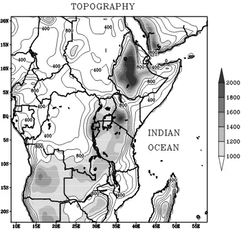
Figure 2.1: Topographical features of the outer domain, with areas higher than 1000m shaded
2.2 Model Validation Data
2.2.1 Gauge-observed rainfall data
The rain gauge observations network over East Africa is quite sparse. Furthermore, the available data are also riddled with numerous gaps in both space and time. These limitations in the quantity and quality of in situ observations impose substantial constraints on diagnostic studies of the regional climate (rainfall) variability. In this study monthly mean rainfall data were available from 136 stations (unevenly distributed) over East Africa during the 1961-1990 period and has been used to construct observed rainfall climatology. For the period after 1990, the stations with complete data are even fewer.
To evaluate the simulated diurnal variability of the climate over the lake basin, daily rainfall observations from near-shore stations have been used. Consistent daily rainfall data from five lakeshore stations; Kisumu, Bukoba, Entebbe, Jinja and Mwanza have been obtained from the Drought Monitoring Center data archive in Nairobi. However, no in situ observations are available over the Lake Victoria. Hence, to complement the available gauge-observations, satellite data have been used as well. These proxy datasets are described in the following sub-sections.
2.2.2 Climate Prediction Center Merged Analysis of Precipitation Data (CMAP)
MSU) while recent gauge-based rainfall estimates are produced by the Global Precipitation Climatology Centre (GPCC). GPCC estimates exists over land from 1986 to the present and incorporates rainfall from 6700 stations worldwide that are statistically interpolated on to 2.5º × 2.5 º grids (Xie and Arkin, 1997). Prior to 1986, the rainfall estimates were acquired from about 5000 gauges collected in the Climate Anomaly Monitoring system of the NOAA Climate Prediction Center ( Xie and Arkin, 1995). Over the oceans no gauge data are available so that the values come solely from satellite estimates. Detailed description of CMAP dataset is available in Xie and Arkin (1996, 997).
2.2.3 Climate Research Unit (CRU TS 2.0) Dataset
The CRU TS 2.0 dataset comprises of 1200 monthly-observed climate for the period 1901-2000 covering the global land surface and have been interpolated onto regular 0.5ox0.5o grid spacing (Mitchel et al., 2005). The dataset contains five climatic variables; precipitation, surface temperature, diurnal temperature range (DTR), cloud cover and vapor pressure. It is a revised and extended version of similar data constructed by New et al. (2000). In the present study only the surface temperature and precipitation variables have been used for model evaluation.
orbit (350km before 2001, and 430km afterwards) and carries a suite of five instruments; precipitation radar, multi-frequency TRMM imager (TMI), multi-frequency visible and infrared (VIRS), lightning imaging sensor, and clouds and earth’s radiant energy system. The TRMM precipitation radar (PR) and passive microwave radiometers builds homogeneous dataset of rainfall rate and vertical structures of precipitating systems over land and tropical oceans.
CHAPTER 3
3 VARIABILITY OF THE GREATER HORN OF AFRICA CLIMATE BASED ON GCM ENSEMBLE SIMULATIONS
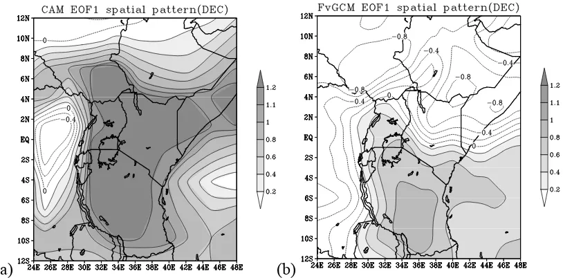
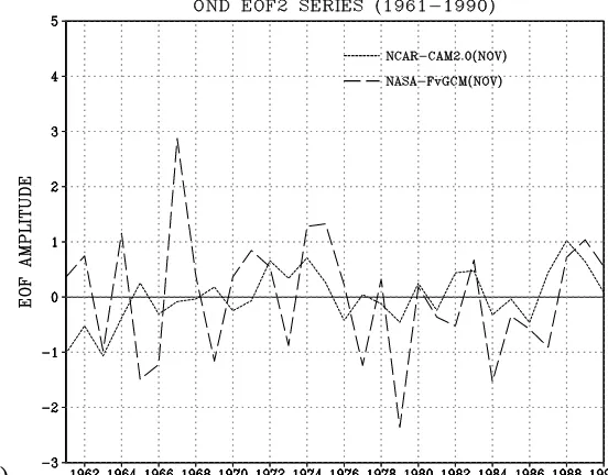
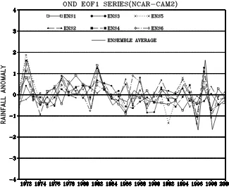
The intra-seasonal, seasonal and inter-annual variability of the Greater Horn of Africa (GHA) climate is investigated based on multi-year ensemble simulations by two GCMs. The GCMs are the eulerian version of NCAR-Community Atmosphere Model (CAM.2.0.1) and the finite volume version of the NCAR/NASA-CCM3. The NCAR-CAM2.0.1 ensemble consists of 15 realizations for 50 years (1948-2001). The NASA-CCM3 data is an ensemble of only two members, each of which covers a period of 30 years (1961-1990). Empirical Orthogonal Functions (EOF) technique has been employed to characterize the dominant and physically coherent modes of spatial and temporal variability of the sub-regional climate during the short rains season (October-December). The spatial and temporal patterns derived from EOF analysis of the two GCM ensembles are compared with CMAP data, CRU data and gauge observations derived from 136 East Africa rainfall stations.
variability is further subjected to dynamical downscaling using the latest version of the ICTP regional climate model (RegCM3) coupled to a 3D lake model (POM) to investigate the regional details of the coupled variability of Lake Victoria Basin and contiguous regions. A brief discussion of some of the GCM studies focusing on the equatorial eastern Africa and/or the GHA sub-region is given in the next section.
3.1 Introduction
The Greater Horn of Africa (GHA) sub-region covering eastern and the Horn of Africa has a distinct climate regime compared to the rest of the continent. The seasonal and inter-annual variability of the sub-regional climate are also characterized by extreme fluctuations, often associated with droughts and floods. However, the inter-tropical convergence zone (ITCZ) that traverses the region twice a year has significant influence on the climatological rainfall pattern. The ITCZ influence is largely responsible for the bimodal rainfall pattern experienced over many parts during March to May (long rains) and October to December (short rains). The inter-annual variability of the GHA climate is mainly associated with perturbations in the global SSTs, especially over the equatorial Pacific and India Ocean basins, and the Atlantic Ocean to some extent (Ogallo, 1988; Nicholson, 1996; Mutai et al., 2000; Indeje et al., 2000; Saji et al., 1999; Goddard and Graham, 1999, among others). In particular, El Nino/Southern Oscillation (ENSO) anomaly patterns have been shown to play a predominant influence on the inter-annual variability of the regional climate (Ogallo, 1988; Indeje et al., 2000).
variability and predictability of the GHA sub-regional climate. GCMs have become useful tools employed to enhance understanding of the variability of the climate system and also to aid in prediction of future climates (McGuffie and Henderson-Sellers, 2001). The phenomenal growth in computer power and capability has also enabled the current versions of GCMs to become sophisticated enough, thus leading to their improved skill in simulating and predicting certain aspects of large scale seasonal and inter-annual climate variability. For, instance, several GCMs can now predict the atmospheric response to SST anomalies associated with El Niño events with lead times longer than two seasons (Zebiak and Cane, 1995, 1997; IPCC, 2001). The improved simulations of some of the large-scale features of tropical rainfall patterns by AGCMs have also been attributed to the close relationship between rainfall and tropical sea surface temperatures (Mechoso et al. 1990).
investigated the month-to-month variability of East African rainfall during the long rains (March-May) and concluded that for this season, unlike the short rains, there were significant month-to-month variations in the response of regional climate to global SST anomalies. However, the simulations were performed for a very limited period of time (four years) that was not sufficient to comprehensively characterize the intra-seasonal and inter-annual variability of the regional climate.
Goddard and Graham (1999) used the German version of the European Commission GCM (ECHAM3) model to study the relative importance of the Pacific and Indian Ocean SSTs on eastern and southern African climate variability. Their study indicated that inter-annual rainfall variability over eastern and southern Africa correlates highly with ENSO as well as SST variability over Indian Ocean. In the simulations in which ECHAM3 was forced alternately with climatological and observed SSTs over the Indian and the Pacific Ocean Basins the study showed that the Indian Ocean SST variability had the dominating role in setting up a dipole precipitation (wet/dry) pattern over eastern and southern Africa. At the same time the variability of Indian Ocean SSTs were also shown to be significantly linked to SST variability over the tropical Pacific Ocean, with the latter leading by three months.
Semazzi, 2000) correct simulations of such ENSO-related fluctuations is a fundamental criterion for evaluating performance of GCMs over the region.
Recently, Behera et al. (2003) have also investigated the impact of the Indian Ocean Dipole mode on East African short rains using a coupled Ocean-Atmosphere General Circulation Model and obtained realistic simulations of the seasonal variability compared to observed climatology. The simulated results also compared quite well to other earlier empirical studies (e.g. Saji et al., 1999, Webster, 1999; Hasternrath et al., 1993; Black et al., 2003, among others). Of particular interest, Behera et al. (2003) showed that about 31% of the Indian Ocean Zonal temperature gradient anomalies or the Dipole Mode Indices (DMI) were associated with warm ENSO events while other DMI events were not necessarily linked to the equatorial Pacific SST anomalies. Regarding rainfall variability over East Africa, the study concluded that unusually wet conditions were experienced mostly when the DMI events coincided with the warm phase of ENSO than in the absence of ENSO events. This conclusion somehow, but not necessarily, concurs with the results of Goddard and Graham (1999) and Black et al. (2003).
analyzing GCM simulations on a regional scale where year-to-year and decade-to-decade differences in the simulated climate are often magnified and may introduce more uncertainty (Wehner, 1998). However, the prohibitive computational expense of performing lengthy climate simulations has often limited the ensemble size utilized in many previous GCM based studies over Africa (e.g. in Ininda, 1998; Goddard and Graham, 1999).
The primary objectives of the present study are:
(i) to assess the performance of two GCMs in simulating the sub-seasonal to inter-annual variability of the GHA climate based on multi-year ensemble simulations.
(ii) to evaluate the range of uncertainty in the ensemble simulations of the intra-seasonal, seasonal and inter-annual variability over the GHA sub-region based on EOF analysis of individual ensembles as well as the ensemble average.
(iii) investigate the probable physical mechanisms associated with the episodic floods of 1961(non-ENSO) and 1997(warm ENSO) years
The data and methods of analysis used in this study are briefly described in the following sub-sections.
3.2 Data and methods of analysis
3.2.1 Observed rainfall and wind data
CMAP is a hybrid of satellite, gauge (and model) data that has been merged using various data assimilation and interpolation techniques (Xie and Arkin, 1996, 1997). A recent study by Schreck and Semazzi (2004) performed EOF analysis using short rains seasonal CMAP data and showed that the data realistically represent the seasonal and inter-annual climate variability of eastern Africa. Hence, the dataset is a reasonable proxy to the relatively sparse gauge observations over the GHA. CMAP data is on a 2.5o x 2.5o uniform grid. CRU data are derived from gauge observations over land areas only and are interpolated on a regular 0.5o x 0.5o grid (Mitchel, et al., 2005). For the evaluation of the circulation patterns in the ensemble simulations, we use the 2.5o x 2.5o NCEP reanalysis data (Kalnay et al., 1996). Detailed descriptions of these datasets have been given earlier in Chapter 2 of this thesis.
3.2.2 NCAR-CAM2.0.1 model ensemble
Stüfing (1981), which is terrain following at the earth’s surface but reduces to pressure coordinate at some point above the surface. The cumulus parameterization scheme for deep convection is based on Zhang et al. (2003). The model also has enhanced physics that includes prognostic treatment of cloud-condensed water to deal more realistically with condensation and evaporation due to large scale forcing. Explicit representation of fractional land and sea-ice coverage is adopted in CAM2.0.1 unlike the earlier versions of the NCAR global atmospheric model (the CCM series) that uses a simple land-ocean-sea ice mask to define the underlying surface of the model. Detailed description of NCAR CAM2.0.1 series can be accessed online at the NCAR website (http://www.ccsm.ucar.edu/models/atm-cam/index.html).
The ensemble data used in the present study comprises of 50-year simulations with 15 realizations. Perturbing the initial surface temperature conditions generated the ensemble members. Details of the ensemble simulations can be found online at the NCAR-Climate Variability website (http://www.ccsm.ucar.edu/working_groups/Variability/index.html). This study takes advantage of this large ensemble size to evaluate the performance of the GCM in simulating the climate of the GHA sub-region. It is often not possible to generate such large GCM ensemble size, due to the prohibitive computational costs involved.
3.2.3 Finite volume NCAR/NASA-CCM3 ensemble
it uses the mass conserving finite element volume dynamics (Lin and Rood, 1996; Lin et al. 2004). The horizontal resolution is 1o latitude x1.25o longitude grid coordinates. Hybrid vertical coordinate system is used with a total of 18 levels.
The two ensembles were both run using observed SSTs, sea ice distribution and GHGs. The first ensemble member was initialized with the climatological January fields while the second with the fields obtained one week after the first run (Coppola and Giorgi, 2004). A detailed description of the finite volume version of CCM3 can be found in Lin and Rood (1996) and Lin et al., (2004) while the ensemble simulations are described in more detail in Coppola and Giorgi (2004).
3.3 Empirical Orthogonal Functions (EOF) technique
CMAP is the primary data used for the evaluation of the spatial and temporal patterns of the EOF modes constructed from the CAM2.0.1 ensemble due to the spatial superiority of CMAP (since it incorporates satellite observations). Besides, CMAP data have approximately the same spatial resolution as the CAM2.0.1 model used to generate the ensemble dataset. 3.4 Results and discussions
3.4.1 GCM ensemble and observed rainfall climatology
First, the ability of the two GCMs (NCAR-CAM2.0.1 and NCAR/NASA-CCM3) to represent the climatological rainfall pattern over the GHA sub-region is evaluated. The rainfall climatologies are derived for the 1961-1990 base period for both GCMs and CMAP data. However, CMAP climatology has been derived for 22 years (1979-2000) due to the limitation of the period of data availability. CMAP data, which merges satellite and gauge observations, is only available since 1979. Nevertheless, due to its spatial superiority it has been shown to be a suitable surrogate for diagnosing the climate variability over equatorial eastern Africa (Schreck and Semazzi, 2004).
a) (b)
(c) (d)
3.4.2 Latitude-time evolution of rainfall during the short rains season
Figure 3.2 show comparisons of latitude-time evolution between the two GCMs ensemble averages and observed rainfall derived from CMAP and CRU datasets during the short rains season of 1988. The short rains season in 1988 had near normal climatological conditions, especially over equatorial East Africa (Ininda, 1998, Indeje et al., 2000). The mean monthly rainfall (mm/day) for five months (September through January) is averaged between 28oE to 43oE longitudes. The north-south extent of the domain ranges from 10oS to 10oN. The area mainly covers land areas, but also includes a small section of the western Indian Ocean. The averaging period includes one month before and one month after the normal onset (October) and cessation (December) of short rains over most parts of eastern Africa in order to examine the latitude-time evolution of the seasonal rainfall(short rains) over the full length and breadth of our study domain. The data over oceans are excluded since the observed datasets (CRU and Wilmott) used to evaluate the GCMs only have data over land areas only.