ABSTRACT
Mountjoy, Daniel Neal. Perception-Based Development and Performance Testing of a
Non-Linear Map Display. (Under the direction of Dr. Sharolyn A. Converse and Dr.
James R. Wilson.)
The use of non-linear display methodologies has been successfully
demonstrated in a number of text-based and simple, graphic network applications;
however, most studies have focused on computational efficiency with very little
attention to human perceptual limitations. While the benefits of non-linear displays
are purported to be due to additional context with no loss of required detail, reports of
end-user performance gains have been limited at best. This research entailed the
design of a non-linear tactical map display, where the distortion parameters were
based upon empirical test results of navigation-related tasks combining various scales
and distortion techniques. A total of three experiments were conducted: two to define
the non-linear display parameters, and the third to attempt to validate the display
through a performance test using military participants. Results indicate that additional
scales can indeed be combined on the same map surface with no significant penalty in
navigation accuracy. However, there may be a response time difference depending on
the particular distortion technique applied. A modified fisheye distortion proved to be
better suited to this task environment than a Cartesian bifocal distortion. Performance
testing versus a traditional, pan and zoom display interface yielded no differences in
PERCEPTION-BASED DEVELOPMENT AND PERFORMANCE TESTING OF A NON-LINEAR MAP DISPLAY
by
DANIEL NEAL MOUNTJOY
A dissertation submitted to the Graduate Faculty of North Carolina State University
in partial fulfillment of the requirements for the Degree of
Doctor of Philosophy
INDUSTRIAL ENGINEERING
Raleigh
2001
APPROVED BY:
___________________________ ___________________________ Celestine A. Ntuen, Ph.D. William P. Marshak, Ph.D.
DEDICATION
To a man who always offered me encouragement and
inspiration; a man who rarely missed a Little League
game, band concert, choir concert or football game;
Someone I truly miss.
I love you, Dad.
~
Thomas Earl Mountjoy
BIOGRAPHY
Daniel Neal Mountjoy received the B.S.E. degree in Systems Engineering
(Human Factors) from Wright State University in 1989, and subsequently the M.S.E.
in the same field in 1991, also from Wright State University. His Master’s level work
focused on human knowledge representation, in particular, the validation of a model
of knowledge representation proposed by Dr. Richard J. Koubek (currently the Chair
of the Department of Biomedical and Human Factors Engineering at Wright State).
Since receiving the M.S.E. degree, Daniel has worked for two different companies
performing research primarily funded by the United States Department of Defense:
Anthropology Research Project, Incorporated (1991-1993) and Sytronics Incorporated
from 1993 to 2000. On the physical side of human factors, his work has entailed both
traditional and 3-D anthropometric data collection and modeling for U.S. Air Force
and Army clothing and workstation design projects. Daniel has spent the last four
years exploring advanced display methodologies aimed at improving information
transfer to Army commanders on the digitized battlefield of tomorrow. One such
ACKNOWLEDGEMENTS
I would first like to thank my committee members, Dr. Shari Converse, Dr.
James Wilson, Dr. Celestine Ntuen, Dr. William Marshak, and Dr. Cathy Zimmer, for
all their valuable help in piecing this research together through their combined
expertise in engineering, display evaluation, experimental and cognitive psychology
and statistics. Dr. David Kaber deserves special recognition for the great deal of time
spent offering his advice on the statistics as well as the write-up. I certainly would
like to thank my employer through most of this, Sytronics Incorporated, for their
financial backing, for without that I would never have considered going back to
school. My former boss, Dr. (Bill) Marshak deserves a second mention since I think it
was his grand scheme that moved me to North Carolina and got me into this whole
mess to begin with. Seriously, though, it was Bill that encouraged me to pursue the
Ph.D., and his urging (nagging?) and guidance was crucial in making that happen. I
would like to express my sincere gratitude to Mary Wesler who went out of her way
(all the way to New York) to assist in the data collection effort at the U.S. Military
Academy – her assistance was invaluable. Speaking of the Academy, Lieutenant
Colonel Larry Shattuck, Department of Behavioral Sciences and Leadership, arranged
for the final data collection to take place there, advertised for subjects, and made sure I
ended up with enough data points. Major James Merlo, Captain John Graham, and
Captain Steve (Mark) McMillion at the USMA all contributed greatly in the subject
Laboratory for believing (at least a little bit!) that this research was indeed worth
looking into. It was ultimately his call that let the West Point trip fall into place. I
would especially like to thank my parents for their love and encouragement through
the years. They taught me about the really important things in life. Finally, thanks to
my wife of ten years, Amanda, and our sons, Bryant and Joseph – I know the last few
years haven’t been particularly fun for them. Sometimes nights were late, sometimes
schedules and plans were interfered with, but they didn’t complain…too much. I love
TABLE OF CONTENTS
Page
LIST OF TABLES ... x
LIST OF FIGURES... xi
1. INTRODUCTION... 1
1.1 Identification of the Problem ... 2
1.2 Current Approaches... 3
1.3 Proposed Solution ... 4
1.4 Research Objectives and Approach... 6
1.5 Organization of the Dissertation ... 7
2. LITERATURE REVIEW... 8
2.1 Non-Linear Display Research ... 8
2.2 Distortion Algorithms ... 9
2.3 Graphical Perception ... 15
2.3.1. Weber’s Law ... 16
2.3.2. Stevens’ Law ... 17
2.3.3. Discussion of Graphical Perception ... 18
2.4 Situation Awareness and Performance Testing... 18
2.4.1. Definitions and measurement of situation awareness ... 21
2.5 Implications of Literature Review / Motivation for Proposed Research ... 22
3. EXPERIMENT I: THE EFFECT OF SCALE CHANGE ON MILEAGE ESTIMATION ... 24
3.1.1 Subjects ... 24
3.1.2 Apparatus ... 24
3.1.3 Experimental Design ... 25
3.1.4 Stimuli ... 26
3.1.5 Procedure... 28
3.2 Results ... 30
3.2.1 Mileage Estimation Accuracy ... 30
3.2.2 Response Time ... 31
3.2.3 Perceived Workload ... 33
3.2.4 Individual Differences... 34
3.3 Experiment I Discussion ... 35
4. EXPERIMENT II: THE EFFECT OF DISTORTION TYPE ON MILEAGE AND HEADING ESTIMATION ... 38
4.1 Method ... 38
4.1.1 Subjects ... 38
4.1.2 Apparatus ... 39
4.1.3 Experimental Design ... 39
4.1.4 Stimuli ... 40
4.1.5 Procedure... 43
4.2 Results ... 47
4.2.1 Mileage Estimation Error ... 47
4.2.2 Heading Estimation Error ... 49
4.2.4 Heading Estimation Response Time ... 52
4.2.5 Workload Ratings... 53
4.2.6 Individual Differences... 53
4.3 Experiment II Discussion ... 54
5. EXPERIMENT III: PERFORMANCE TEST ... 59
5.1 Method ... 60
5.1.1 Subjects ... 60
5.1.2 Apparatus ... 60
5.1.3 Experimental Design ... 61
5.1.4 Stimuli ... 61
5.1.5 Procedure... 64
5.2 Results ... 66
5.2.1 Mileage Estimation Accuracy ... 67
5.2.2 Mileage Estimation Response Time... 68
5.2.3 Heading Estimation Accuracy... 68
5.2.4 Heading Estimation Response Time ... 69
5.2.5 Number of Detected Critical Events ... 69
5.2.6 Critical Event Detection Response Time ... 70
5.2.7 Perceived Workload ... 71
5.2.8 Number of Required Interface Manipulations ... 71
5.2.9 Individual Differences... 72
6. GENERAL DISCUSSION AND CONCLUSIONS ... 75
6.1 Recommendations for Future Work... 76
7. REFERENCES... 80
8. APPENDICES... 83
8.1 Appendix A: North Carolina State University Informed Consent Form ... 84
8.2 Appendix B: Pre-Data Collection Information Survey ... 87
8.3 Appendix C: Experiment II Target Distribution ... 89
8.4 Appendix D: Matlab Code for Bifocal Non-Linear Map Generation ... 91
8.5 Appendix E: Matlab Code for Modified Fisheye Non-Linear Map Generation... 95
8.6 Appendix F: Task Description Provided to Experiment III Participants ... 98
8.7 Appendix G: Experiment I SAS Code and Output ... 100
8.8 Appendix H: Experiment II SAS Code and Output ... 105
8.9 Appendix I: Experiment III SAS Code and Output ... 113
LIST OF TABLES
Page
Table 2.1 Example exponents for Stevens’ Law... 18
LIST OF FIGURES
Page
Figure 2.1 Standard fisheye distortion ... 10
Figure 2.2 Uniform grid ... 11
Figure 2.3 Example bifocal grid... 11
Figure 2.4 Example grid transformed into polar coordinates outside a designated linear area ... 12
Figure 2.5 A standard 1:67K scale map of the Baghdad, Iraq area... 14
Figure 2.6 Mockup of the map from Figure 2.5 after undergoing a Cartesian demagnification (0.5X) in areas outside of grid location 10... 15
Figure 3.1 One-Inch Linear scale grid ... 26
Figure 3.2 Half-Inch Linear scale grid ... 26
Figure 3.3 Quarter-Inch Linear scale grid... 27
Figure 3.4 Half-Inch Bifocal and Half-Inch True Bifocal grid ... 27
Figure 3.5 Quarter-Inch Bifocal grid... 27
Figure 3.6 Modified Fisheye grid... 28
Figure 3.7 Mean mileage estimation error for each of the twelve target pairs ... 30
Figure 3.8 Mean response times for the mileage estimation task ... 31
Figure 3.9 Mean response times for each target pair across the seven scale types .... 32
Figure 3.10 Interaction between the scale types and the target pairs on estimation response time... 33
Figure 3.11 Interaction between the scale types and target pairs... 33
Figure 3.12 Mean performance ratings for mileage estimation task... 34
Figure 4.2 Distorted stimulus employed for the Cartesian Bifocal treatment group . 41
Figure 4.3 Distorted stimulus employed for the Modified Fisheye treatment group. 42
Figure 4.4 The angle estimation trainer ... 43
Figure 4.5 Distribution of targets for Experiment II ... 46
Figure 4.6 The effect of Target Pair on mileage estimation error... 48
Figure 4.7 The interaction between Distortion Type and Target Pair on mileage estimation error ... 48
Figure 4.8 The Distortion Type x Target Pair interaction displayed as linear trend lines ... 49
Figure 4.9 The effect of Target Pair on heading estimation error... 50
Figure 4.10 Response times for mileage estimations across all targets ... 51
Figure 4.11 Response times for mileage estimations to off-axis targets... 51
Figure 4.12 The effect of Target Pair on mileage estimation response time ... 52
Figure 4.13 The effect of Target Pair on heading estimation response time ... 52
Figure 5.1 Mock battlefield map ... 62
Figure 5.2 The control group’s display interface ... 63
Figure 5.3 The Modified Fisheye Distortion display interface ... 64
Figure 5.4 The effect of Target Location on mileage estimation accuracy... 67
Figure 5.5 The effect of Target Location on mileage estimation response time... 68
Figure 5.6 The effect of Target Location on heading estimation accuracy... 69
1. INTRODUCTION
At the height of the Cold War in 1968, the U.S. Army consisted of roughly
1,570,000 active personnel (U.S. Department of Defense, Directorate for Information
Operations and Reports, Statistical Information Analysis Division, 1995). During the
1989 fiscal year (following the toppling of the Berlin Wall and the declared end of the
Cold War) the Army began a major downsizing effort with an end result of 495,000
present-day active personnel (West and Reimer, 1996). As one might expect, along with
the decline of the “communist threat” military downsizing has occurred partly due to
budgetary constraints, and because of political and philosophical changes in the manner
in which the United States Government views its role in world peacekeeping (which is
influenced, in theory at least, by the changing views among the U.S. population as a
whole).
Due to its relative lack of numbers, the U.S. military has now recognized more
than ever the importance to win what is known as the information war; that is, in basic
terms, gaining an upper hand on the enemy by knowing more about the battlefield and
knowing it sooner (real-time situation awareness). The Army must be sleeker, smarter,
and faster than the enemy to maintain a high level of effectiveness. This idea has been
put into motion within the constructs of the future Army, Force XXI (U. S. Department of
the Army, Training and Doctrine Command, 1994).
As part of the Force XXI effort, the Army is currently funding research aimed at
the development of advanced sensors, data transmission/telecommunication, and
information display. The bottleneck in this scheme is the display area along with the
Concepts such as virtual reality, voice recognition software, intelligent data filters, tactile
displays, and gesture recognition are currently being explored as possibilities to improve
the soldier-display interface. The overall goal of the research is to enhance soldier
performance through reduced workload and increased situation awareness.
Unfortunately, the past decade of digitization research has not yet delivered on the
promise of digital advantages. One of the key difficulties rests in the bandwidth
requirements of newly developed visual displays (i.e., the required data throughput for
these displays to operate reliably and correctly). Due to lack of sufficient display
bandwidth, visual information is sometimes fragmented or simply cannot be displayed at
all. One innovative approach to reducing bandwidth requirements is the exploitation of
the elasticity of the display surface. Elasticity, as used here, is the ability to
simultaneously display more than one scale on an electronic display – a sort of stretching
or compression of the spatial information that is decidedly non-linear in its nature. The
non-linear display of map information is the focus of this research.
1.1 Identification of the Problem
Advances in information technology and subsequent “digitization of the
battlefield” is providing an impetus to move away from the present-day world (where
commanders and their staff typically rely on large paper maps for battle planning)
towards digital maps displayed on computer monitors. For battle planning and situation
awareness, brigade level commanders typically utilize a 1:250,000 scale paper map
the question. The incorporation of large electronic displays is also limited by the
vehicle’s interior dimensions. This all points to the need to develop new methods to
present large amounts of visual information in smaller, pixel-limited displays.
Even in tent-based operations such as a brigade-level tactical operations center
(TOC), the present technology advancement does not allow for a large screen display
suitable for this type of application (i.e., portable, rugged, high resolution). Digital
display systems in the field today utilize a 35” (at most) diagonal monitor, with 20” or
17” monitors more common.
Furthermore, electronic display resolutions are typically 72 dpi (dots per inch) or
less. Color displays can range up to 100 dpi, while monochrome displays may reach 300
dpi. When compared to a paper map’s resolution of at least 9600 dpi, it is easy to see that
detail is lost when electronic displays are used in an attempt to recreate the same area
coverage.
1.2 Current Approaches
A typical method used to counter this problem is to provide a map of a scale of
choice, and through the use of scroll bars, allow the user to pan around the map to
explore various areas of interest. If a more or less detailed view is desired, maps of
different scales can be selected. When using this methodology, however, updated
information may be missed if it is not in the visible portion of the screen, and as a direct
result, it becomes difficult to form an accurate mental image of the entire space. The user
must integrate the images from the various panned scenes in order to have a clear
There is evidence to suggest this is a difficult task (Henry & Hudson, 1991; Tolsby,
1993). Similar results can be expected when a magnified image area is displayed on top
of or beside an original image. An additional drawback of simple magnified images is
the possibility that the magnified window may occlude important underlying information
– information that was once peripheral to the magnified area. Still another approach
sometimes taken is to tile the image over multiple displays, where individual monitors
display different pieces of the map. Beyond the issues of bandwidth and pure monetary
cost, this method can result in a “French window effect”, where information can be lost
or fragmented due to the distraction caused by the transition space between displays
(Schneiderman, 1992). Given these integration issues (cognitive and otherwise), it is
suggested that a single-window display should be developed that provides detail (focus)
where needed, but at the same time provides enough information about outlying areas
(context) to enhance situation awareness (the situation awareness construct will be more
fully addressed in Section 2.4).
1.3 Proposed Solution
Brigade-level Army commanders are primarily concerned with their area of
responsibility (AOR) and require detailed information in that area. Outside of the AOR,
only a lower-detailed “big picture” is necessary. A display methodology to explore, then,
is to provide a multiple-scale map display where only the area of current interest is
displayed in a higher or magnified scale, and areas outside are de-magnified exploiting
expanded area represented in the single display. This display technique is often referred
to as non-linear magnification or distortion-oriented display, and has been explored in
areas such as geographical information systems (GIS), workspace awareness, large graph
viewing, and hierarchical network navigation (Anderson, Smith & Zhang, 1996; Gutwin,
Greenberg & Roseman, 1996; Sarkar & Brown, 1992; Schaffer, Zuo, Greenberg,
Bartram, Dill, Dubs & Roseman, 1996). A nice survey of applications in the information
visualization domain is provided by Herman, Melancon & Marshall (2000).
A rather large body of research in this field revolves around text-based,
groupware applications where multiple individuals may be simultaneously working on
the same document. In these applications, text in the particular area of interest is
magnified, while others’ work areas are de-magnified (see for example, Greenberg,
Gutwin & Cockburn, 1996a; Greenberg, Gutwin & Cockburn, 1996b; Greenberg &
Gutwin, 1995).
Non-linear display techniques have never been pursued for the display of military
tactical situation maps. Furthermore, most existing references in this area describe
various display techniques and computing algorithms, but have primarily focused on
computing efficiency – very little has been reported on the associated human
performance benefits. While the following quote from Herman et al. (2000) is directed at
the information visualization domain in particular, it appears to hold true throughout the
literature on the benefits of non-linear display work in general:
science have practical applications at this time and very few usability studies have been done” (p.28).
It certainly stands that, while maps can be distorted a great deal computationally,
there is likely some perceptual limit to how much (and what type of) distortion can be
tolerated without sacrificing user performance. It is, therefore, critical that human
perceptual and cognitive abilities are addressed from the start in the development of
tactical mapping systems.
1.4 Research Objectives and Approach
For the purposes of this research, the operating definition of a non-linear map is
as follows: A non-linear map is one in which two or more scales and/or coordinate
systems are combined within a single map product. There are two main questions to be
addressed by this research. First, if a non-linear map display is to be developed, what
type of distortion effects will lead to the least decrement in spatial interpretations (such as
navigation task performance)? This question is asked since two primary uses of maps are
distance and heading estimation. It is suggested, then, that in the construction of a map
tool, one should ensure that the performance of these tasks is not detrimentally affected.
Second, can non-linear map displays facilitate the monitoring of battlefield events better
than traditional pan and zoom map displays?
To answer the two primary questions as stated above, three experiments were
conducted. Experiments I and II were basic perception studies meant to determine the
linear mapping system versus a more traditional pan and zoom approach. The
methodology and results of each of these experiments is provided in the three chapters
following the literature review.
1.5 Organization of the Dissertation
The remainder of this dissertation is organized as follows: Chapter 2 contains the
literature review. Chapters 3 and 4 detail the two perception experiments performed to
establish the human-centered design parameters for non-linear maps. Chapter 5 describes
the performance study carried out in an attempt to validate the findings of the perception
experiments. The main portion of the dissertation ends in Chapter 6, which provides a
general discussion and recommendations for further research. References, appendices
2. LITERATURE REVIEW
The literature review is separated into three sections. First, historical research on
the application of non-linear displays is reviewed, followed by a section on
psychophysics and graphical perception – a look at human perceptual abilities in relation
to graphical elements such as line lengths and distance estimations. These are viewed as
important issues in the development of the specific approach taken in this dissertation
research. The third section provides an overview of the concept of situation awareness
along with associated measurement methodologies, and is meant to provide the
foundation to understand the reasoning behind the specific display evaluation paradigm
undertaken here.
2.1 Non-Linear Display Research
Although a non-linear display may be new to military applications, the concept
has been around since at least the mid-1980s when George Furnas presented a “fisheye
view” approach to displaying large volumes of text in computer programs and databases.
According to Furnas (1986) the fundamental motivation was to provide a balance
between local detail and global context (e.g. understanding a single line of code versus
understanding its purpose in the function in which it resides). The fisheye view approach
was a success in this particular application. When tested in a code navigation-related
task, subjects performed better (i.e., provided more correct responses) when using fisheye
views than the standard, “flat” view.
efficient algorithms for generating and displaying fisheye views, and no results of their
own performance testing were presented. However, other researchers have carried out
performance tests in this area. For example, Schaffer, Zuo, Greenberg, Bartram, Dill,
Dubs & Roseman (1996) found favorable results when using a fisheye display to navigate
hierarchically clustered networks such as a telephone network. Subjects were asked to
find breaks in lines, and to “repair” the network by re-routing lines to other nodes in the
network. The fisheye display was tested versus a full zoom approach where subjects
could alternately zoom and un-zoom to locate problems. Subjects took less time to
perform the task and required less navigation (zooming and un-zooming) when using the
fisheye display. Schaffer et al. suggest that better performance was due to the greater
context provided in the fisheye views.
2.2 Distortion Algorithms
Although everything discussed to this point has been labeled “fisheye” display,
there are, in fact, several different algorithms available to generate various types of
distortion effects. Leung and Apperley (1994) provide a comprehensive guide to
classifying various distortion-oriented presentation techniques along with example
functions used to generate them. Depending on the intended application, one type of
distortion may be better suited than another. Two major types of transformation
functions exist: continuous and discontinuous.
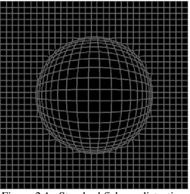
The fisheye display is generated by a continuous transformation function where a
selected display area is magnified, but none of it is held completely in focus (see Figure
focus. Outlying areas (depending on the characteristics of the transformation function)
are de-magnified, and can either be in or out of focus.
Figure 2.1. Standard fisheye distortion. (Source: Keahey, 1998).
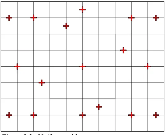
In addition, transformations can be performed using either Cartesian (Figures 2.2
& 2.3) or polar coordinates (Figure 2.4). A variety of non-linear transformations can be
applied to maps that distort the point-to-point distances to reduce map size, but retain the
spatial gestalt of the situation. The first is the bifocal display (Spence & Apperley, 1982),
which differentially magnifies map center and surround. For illustration purposes, a
linear grid (Figure 2.2) is distorted using the bifocal approach as shown in Figure 2.3.
While the relative positions of the crosshairs are maintained, the increased coverage area
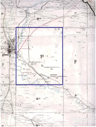
(i.e., context) of the grid is readily apparent. Another mockup of the bifocal distortion
was applied to a real map (Figure 2.5) with the resulting transformed map shown in
Figure 2.6. Notice that the map is quite a bit smaller in size, but retains the spatial
Figure 2.2. Uniform grid.
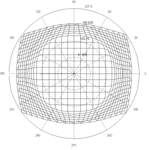
Figure 2.4. Example grid transformed into polar coordinates outside a designated linear area (also known as the modified fisheye distortion).
An alternative compression algorithm similar to the fisheye concept uses polar
coordinates to modify the map based on location relative to the map center (Figure 2.4).
This map has a linear center and a surround collapsed about it. Although distances are
distorted, the polar transform preserves directional relationships between the center and
surround. This is referred to as a “modified fisheye” distortion (Mountjoy & Marshak,
1998).
Several distortion techniques have been described in this section, and some have
The challenge and goal of this research, then, is the determination of which distortions (if
any) are best suited for use in mapping applications, specifically those used in tactical
environments. The specific research questions to be addressed are outlined later in this
Figure 2.6. Mockup of the map from Figure 2.5 after undergoing a Cartesian demagnification (0.5X) in areas outside of grid location 10.
2.3 Graphical Perception
Before one can determine the effect of combining multiple scales on a single map
surface, there must be some knowledge regarding human abilities to estimate distances
and headings (or angles) in the more usual, linear sense. This section provides a brief
2.3.1. Weber’s Law
Arguably one of the first derived and fundamental laws of human perception,
Weber’s Law (Weber, 1834) describes the relationship between the intensity of a
stimulus and the percentage of change in intensity necessary for detection (or, the just
noticeable difference – JND). In particular, the magnitude of the JND is said to be a
constant percentage of the stimulus intensity, so that the greater the stimulus intensity,
the greater the magnitude must change before a change in intensity is noticed. Expressed
mathematically
JND = KS,
where S is the magnitude of the stimulus, and K is a constant called the Weber fraction
(Goldstein, 1984).
While originally formulated through experiments with hand-held weights, the law
has been shown to hold for a variety of human senses, so long as the stimulus intensity is
not too close to the threshold or extremely large (Goldstein, 1984; Foley & Moray, 1987;
Matlin, 1988; Bennet, Nagy & Flach, 1997). While no literature has been found
describing its direct relationship to judged distances per se, Weber’s Law has been shown
applicable in detecting differences in line lengths (Cleveland, 1985). Baird (1970)
reports line length JND values in the range of three to five percent. Since judging the
distance between two objects can simply be viewed as judging the length of an imaginary
line between them, it seems logical to assume the same perceptual relationship exists for
2.3.2. Stevens’ Law
Extensive research by Stevens (1957) has shown that, when asked to judge the
magnitude of a particular stimulus when compared to a standard, an individual’s
perceived scale equals the actual scale raised to some power. Stevens’ Power Law, as
this relationship is sometimes known, is expressed mathematically as
p(x) = cxβ,
where x is the magnitude of a standard stimulus, p(x) is the perceived magnitude, and c is
a constant. If β > 1, the perceived magnitude grows faster than the magnitude of the
stimulus, and if β < 1, the perceived magnitude grows more slowly than the magnitude of
the stimulus.
In the case of judging line lengths, β has been shown to range from 0.89 to 1.1
(Baird, 1970; Cleveland, 1985; Foley & Moray, 1987). In other words, humans tend to
be quite good at length estimations. Although a β value was not computed, Cleveland
(1985) reported that angle judgments are generally worse than length judgments.
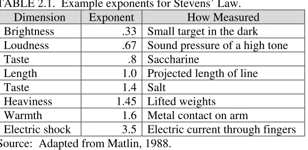
Example exponents for several different stimuli along with how they were measured are
TABLE 2.1. Example exponents for Stevens’ Law.
Dimension Exponent How Measured
Brightness .33 Small target in the dark
Loudness .67 Sound pressure of a high tone
Taste .8 Saccharine
Length 1.0 Projected length of line
Taste 1.4 Salt
Heaviness 1.45 Lifted weights
Warmth 1.6 Metal contact on arm
Electric shock 3.5 Electric current through fingers
Source: Adapted from Matlin, 1988.
2.3.3. Discussion of Graphical Perception
Psychophysical relationships of numerous stimulus types have been studied for
many decades, and data have been compiled to describe them mathematically. It can be
seen that in cases where line lengths are judged, humans tend to be quite accurate.
Perhaps this can be attributed to our frequent experience with rulers and other measuring
instruments (Goldstein, 1984). Since the need to combine more than one scale (not to
mention coordinate systems) on a single measuring device has not historically been an
issue, the perceptual effects of doing so are, at this point, unknown. This is the first
research question addressed in this dissertation.
2.4 Situation Awareness and Performance Testing
While spatial and angular relationships between specific entities are important, it
is also important to provide a more global view of the battlespace (i.e., contextual
information), such that a commander can maintain an accurate mental image of
Unit locations are symbolized on the map, and are updated throughout the course of the
battle. For all intents and purposes, it serves as the commander’s window into the
battlefield – the fundamental visual resource required for maintaining so-called situation
awareness. It is this type of map on which the non-linear distortions will be applied. It
follows, then, that a critical piece of this research is the performance testing of the
non-linear display to determine if such a concept will indeed enhance user performance
through the presentation of greater contextual information.
Perhaps the most important issue in the use of non-linear displays is how they
may affect a commander’s awareness of the important elements and events on the
battlefield (battlefield awareness). It is quite possible that non-linear map displays can
enhance battlefield awareness since they have the ability to display a greater amount of
real estate in the equivalent standard display space. However, if a greater amount of
effort is required in the interpretation of unit locations, for example, the increase in
workload associated with use of a distorted map may outweigh the benefits of additional
viewing area.
The concept of battlefield awareness is theoretically encompassed in the construct
of situation awareness (SA). Situation awareness is a concept that has exploded
throughout human factors literature in recent years, particularly in aviation and military
domains (see, for example,Adams, Tenney & Pew, 1995; Endsley 1995a; Endsley
1995b; National Research council, 1997; Sarter & Woods, 1991; Sarter & Woods, 1995).
While seemingly a research hotbed, it is a topic surrounded in controversy since there is
new “buzzword” attached to the same perception and cognition research that has been
performed for decades.
While a single-most accepted definition does not exist, researchers interested in
SA generally agree it is more than simply knowing what elements are present in the
environment of interest. It also has a great deal to do with the meaning of those elements,
both in the present and future states of events (National Research Council, 1997). By this
description, it should be obvious why the construct of situation awareness is an important
issue in a combat environment. A commander must make critical decisions based upon
his or her understanding of current state of affairs on the battlefield, as well as projections
of possible enemy courses of action and their predicted effects on the current friendly
mission.
The intent of bringing the SA topic into discussion here is not necessarily to
advocate any particular definition as being the best, nor is it to argue whether it is a new
phenomenon. Rather, it is simply the author’s opinion that the concept is useful as a term
descriptive of a type of research – a research genre, perhaps. Because of the controversial
nature of the subject, this research will address individual performance components, and
will eventually leave the SA label behind. However, before abandoning SA completely,
it is important to understand how researchers attempt to measure SA. In other words,
what types of subjective and objective performance measures are generally taken to
2.4.1. Definitions and measurement of situation awareness
According to Adams, Tenney & Pew (1995, p. 85), “situation awareness refers to
the up-to-the-minute cognizance required to operate or maintain a system.” Sarter &
Woods (1991, p.52) define SA as “the accessibility of a comprehensive and coherent
situation representation which is continuously being updated in accordance with the
results of recurrent situation assessments.” A widely published supporter of SA
research, Endsley (1995a, p.37) has provided the following general definition: “Situation
awareness is the perception of the elements in the environment within a volume of time
and space, the comprehension of their meaning, and the projection of their status in the
near future.” She breaks this definition down into three hierarchical levels of SA: Level
1 SA is described as the perception of the elements in the environment; Level 2 SA is the
comprehension of the current situation; and Level 3 SA is the prediction of future
states/events based upon knowledge of the first two SA levels.
To measure SA, Endsley (1995b) has developed the Situation Awareness Global
Assessment Tool (SAGAT), which she claims to be a global measure of all SA elements
based upon comprehensive assessments of operator SA requirements. SAGAT includes a
number of queries regarding Level 1, 2 and 3 SA components, and considers system
functioning as well as external environment features. SAGAT employs a “freeze
technique” where the simulation is halted (and screens blanked) during queries. While
this is done to avoid interference of the queries with normal operator performance, a halt
in the simulation would seem to have a similar interference effect.
Other SA measurement techniques include subjective ratings like the Situation
1995b), and the Subjective Workload Dominance (SWORD) measure (Vidulich, 1989).
SART allows operators to rate system designs based upon the perceived amount of
attention required, the amount of attention resources available, and their understanding of
the task. SWORD requires users to make a number of pairwise comparisons between
competing display designs regarding the degree to which one display provides SA versus
the other (Endsley, 1995b). A drawback of subjective ratings is that, although ratings
may correlate with performance measures, it is unclear whether the SA ratings are
influenced by task performance, or task performance is caused by a particular level of
SA. In other words, a cause and effect relationship cannot be positively concluded (see
Flach, 1995 for an in-depth discussion regarding the dangers of assuming SA to be a
causal agent).
Because of the uncertainty in defining SA, particularly as a directly measurable
variable, and since SA is generally thought to be positively correlated with performance,
traditional performance measures will be recorded during this research effort. Further,
since mental workload is generally associated with available attention resources,
subjective workload ratings will also be employed.
2.5 Implications of Literature Review / Motivation for Research
Of all of the reviewed literature dealing with the topic of non-linear display
magnification, few articles deal with end-user performance as a primary concern. Most
tend to revolve around the programming techniques utilized to create the distortions.
enhanced performance. However, historical applications have generally been text-based
or limited to simple graphics such as network diagrams.
Can the same positive results be expected when non-linear distortions are applied
to a tactical situation map? It seems perfectly reasonable to believe so, but given the
dangerous consequences involved due to the volatile operating environment in which
these tactical maps may be used, it is critical that the distortion parameters be based upon
human perceptual abilities, not simply software know-how. A host of work has been
performed in psychophysics to show that humans are fairly accurate judges of length, and
to a lesser degree, angles. However, since there is no known literature that documents
perceptual abilities in tasks where different scales and/or coordinate systems are
contained in the same visual space, this is the first issue to be examined.
Furthermore, once simple perceptual abilities have been examined, it is necessary
to test the display in a scenario with tasks more similar to those of the intended
end-application – one that involves searching and monitoring for both expected and
unexpected events. The following section outlines the specific procedures implemented
3. EXPERIMENT I: THE EFFECT OF SCALE CHANGE ON MILEAGE ESTIMATION
The purpose of this experiment was to determine the effects of map scale
(single-scale versus multi-(single-scale) on mileage estimation ability. That is, are the errors in mileage
estimation any worse when using multi-scale maps than those when using standard,
single-scale maps? Three hypotheses are addressed in Experiment I:
Hypothesis 1. The introduction of multiple scales within a single map surface will decrease distance estimation accuracy.
Hypothesis 2.The introduction of multiple scales within a single map will increase distance estimation response time.
Hypothesis 3. The introduction of multiple scales within a single map surface will increase subjective workload during mileage estimation.
3.1 Method
3.1.1 Subjects
A total of 84 individuals (43 men and 41 women) volunteered to participate in
this study. Subjects were a mixture of undergraduate and graduate students studying a
variety of disciplines at North Carolina Agricultural & Technical State University. The
participants’ average age was approximately 23 years old.
3.1.2 Apparatus
All stimuli were presented on a 17” diagonal monitor set to a display resolution of
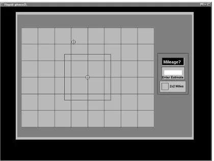
during the experimental trials. The experimental software was created using the rapid
prototyping and simulation package, Rapid (Emultek Ltd., 1997).
3.1.3 Experimental Design
To control for asymmetrical transfer of learning, a between subjects design was
chosen. Subjects were assigned to one of seven treatment groups based on the order in
which they arrived for testing (i.e., first arrival was assigned to first cell, second arrival to
second cell, etc.). The independent variables for this experiment were Scale Type (seven
levels) and Target Pair (twelve levels). The seven levels of Scale Type consisted of the
following: One-Inch Linear, Half-Inch Linear, Quarter-Inch Linear, Half-Inch Bifocal,
Quarter-Inch Bifocal, Modified Fisheye, and Half-Inch True Bifocal. The last display
condition is labeled “True” because it is the only non-linear condition that solely
included non-linear estimations (i.e., in the other three conditions, four of the twelve
different target pairs fell within the linear center). The Half-Inch True Bifocal condition
only contained target pairs that fell across the different scale boundaries. Note that this
seventh condition was added at a later date to ensure that any effects of non-linear
estimations were not diluted due to a combination of linear and non-linear estimations.
The twelve levels of Target Pair consisted of pairs of targets having different inter-target
distances (the targets are described in more detail below).
Dependent variables were Mean Absolute Error, Response Time, the NASA-TLX
measure of Overall Workload, as well as its individual indices of Mental Demand,
Performance, and Frustration Level. While the TLX indices of Temporal Demand,
that these factors would not significantly contribute to overall workload differences in
this task), they were still included in the calculation of the overall workload measure.
3.1.4 Stimuli
The background on which all stimuli were presented consisted of a 1” x 10” grid
divided into either three, five, six, seven, nine or twelve subsections depending on the
experimental treatment. Targets were ¼” diameter white circles with red crosshairs
running through their centers. The grids were located in the center of a 17-inch diagonal
color monitor with a black background. Mileage scales were located beneath the grids
(see Figures 4.1 – 4.6 below).
Figure 3.3. Quarter-Inch Linear scale grid.
Figure 3.4. Half-Inch Bifocal and Half-Inch True Bifocal grid.
Figure 3.6. Modified Fisheye grid.
3.1.5 Procedure
Upon reporting for the experiment, participants were briefed regarding the
purpose and basic procedures of the study, and were then asked to sign a consent form.
Demographic data collected included age, gender and field of study. Each participant
was asked to subjectively rate their mathematical and spatial reasoning abilities on
separate five-point Likert scales (ranging from “Much Below Average” to “Much Above
Average”). They were also asked to disclose if they had prior experience using maps for
activities other than driving, and if so, to explain their experience. The questionnaire can
be found in Appendix B. It is acknowledged that subjective ratings of mathematical and
spatial reasoning aptitude are not terrifically reliable, however, the ratings were included
to see if future research in this area may be warranted.
The experimenter demonstrated the software for the subjects and explained the
task to be performed. Subjects were then given time to become familiar with the
accuracy was most important, but to work quickly. They were informed that accuracy
and response time data were being recorded. Once the individual was satisfied with their
understanding of the task, the experimental trial was initiated.
At the start of the task, the grid and mileage scale(s) were presented in the center
of the screen, where they remained throughout data collection. Following a five-second
waiting period, a randomly selected set of two targets appeared on the grid. Subjects
were to estimate (as accurately as possible) the mileage between target centers based
upon the scale(s) provided below the grid, and key in their estimate using the keyboard.
Response times were recorded as the time lapse between target presentation and the
moment the first key was pressed. When the “Enter” key was pressed, the targets
disappeared, and a five-second inter-stimulus timer began. A different set of targets was
presented following each inter-stimulus break.
The location of targets with respect to the grid was varied (left, right, or center) so
that an equal number of targets appeared in each sector (four in each). A total of twelve
different target pairs were presented exactly twice in a randomized order, resulting in a
total of 24 different mileage estimates. Randomization of target presentation was
controlled to prevent the same pair from appearing immediately following its first
presentation (i.e., the same pair of targets could not appear twice in a row). The two
estimates for repeated target presentations were then averaged to obtain twelve estimates,
one for each target pair. The computerized version of the NASA-TLX workload
assessment technique was administered immediately following completion of the mileage
3.2 Results
Each performance measure (Mileage Estimation Accuracy and Mileage
Estimation Response Time) was analyzed using a mixed-factor analysis of variance
(ANOVA), where Scale Type was the between-groups factor (7 levels) and Target Pair
was the repeated-measures factor (12 levels). Because the administration of NASA-TLX
was performed after the experiment (and hence only one set of measures per subject),
workload indices were analyzed via a single factor (Scale Type) ANOVA in a
between-subjects design. All statistical analysis was performed using the SASsoftware.
3.2.1 Mileage Estimation Accuracy
While the ANOVA results showed no significant differences in mileage
estimation accuracy for Scale Type, F(6,77) = 1.65, p < .15, the effect of Target Pair was
significant, F(11,847) = 28.82, p < .0001. Figure 3.7 shows the relationship between the
mean estimation error and the twelve target pairs. The correlation between the mean
absolute error and the actual distance between targets was also found to be significant, r =
.395, p < .0001. The Scale Type x Target Pair interaction was not statistically significant,
F(66, 847) = 1.12, p < .25.
Mileage Estimation Error for Target Pairs Across All Scale Types
0 0.5 1 1.5 Target 10 Target 1 Target 3 Target 4 Target 2 Target 11 Target 9 Target 6 Target 5 Target 12 Target 7 Target 8 Target Pair
3.2.2 Response Time
Due to a significant interaction between Scale Type and Target Pair, F(66,847) =
1.81, p < .0001, no appropriate error term is available by which to calculate an F-ratio for
Scale Type. In this case, it is necessary to calculate a quasi-F value (designated here by
F) for the effect of Scale Type on response time (Keppel (1982), provides a more
detailed discussion on the use and derivation of this technique). The quasi-F and its
associated degrees of freedom was calculated as F (6,98) = 3.18, p < .007. It is
concluded, then, that the main effect for Scale Type on response time was significant. A
pairwise comparison of means (via Tukey’s Studentized Range Test) revealed the
significant differences occurred between the Half-Inch Linear and Modified Fisheye
conditions (means of 5.9 and 12.6 seconds respectively), as well as the Half-Inch Linear
and Half-Inch True Bifocal (mean = 13.5 seconds) conditions. See Figure 3.8 for a
summary of the response time data for each scale type. The effect of Target Pair was also
found to be significant, F(11,847) = 16.29, p < .0001. This data is summarized in Figure
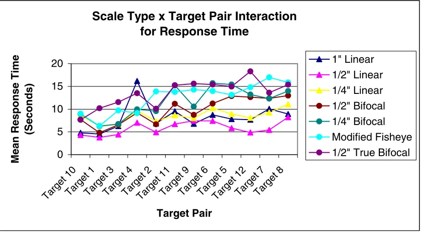
3.9. Figure 3.10 and 3.11 illustrate the nature of the Scale Type x Target Pair interaction.
Distance Estimation Response Times (Mean, Standard Error)
5.9 8.6 9.7 11.5 13.5 12.6 8.2 0.0 2.0 4.0 6.0 8.0 10.0 12.0 14.0 16.0
1" Linear 1/2" Linear 1/4" Linear 1/2" Bifocal 1/4" Bifocal Modified Fisheye 1/2" True Bifocal Scale Type Response Time (Seconds)
Response Time for Target Pairs Across All Scale Types
0 2 4 6 8 10 12 14
Target 10Target 1Target 3Target 4Target 2Target 11Target 9Target 6Target 5Target 12Target 7Target 8
Target Pair
Mean Response Time
(Seconds)
Figure 3.9. Mean response time values for each target pair across the seven scale types. The target pairs were sorted along the x-axis in order of increasing distance between targets.
Scale Type x Target Pair Interaction for Response Time
0 5 10 15 20
Target 10Target 1Target 3Target 4Target 2Target 11Target 9Target 6Target 5Target 12Target 7Target 8
Target Pair
Mean Response Time
(Seconds)
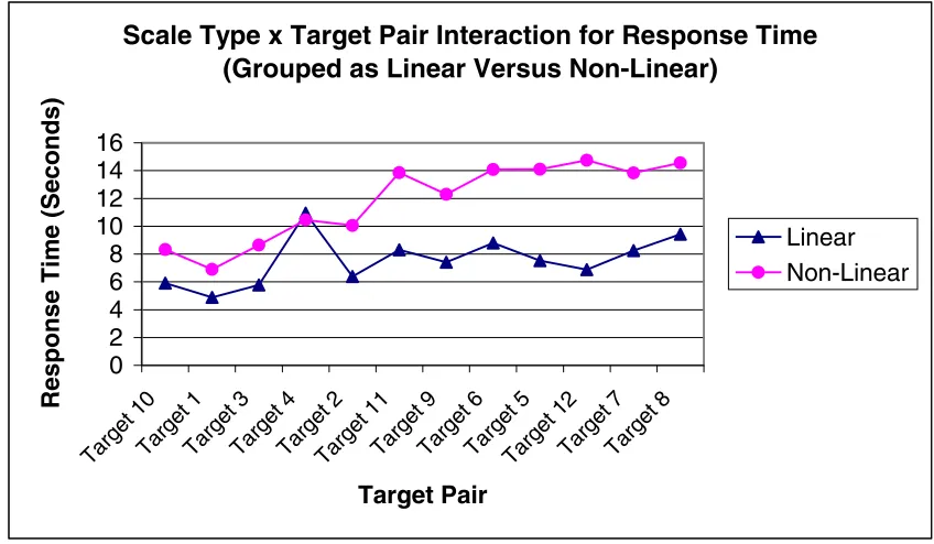
Scale Type x Target Pair Interaction for Response Time (Grouped as Linear Versus Non-Linear)
0 2 4 6 8 10 12 14 16
Target 10Target 1Target 3Target 4Target 2Target 11Target 9Target 6Target 5Target 12Target 7Target 8
Target Pair
Response Time (Seconds)
Linear Non-Linear
Figure 3.11. Interaction between the scale types and the target pairs. To simplify the interpretation of Figure 3.10, displayed response times are combined means of linear and non-linear scale types.
3.2.3 Perceived Workload
Results of the single factor ANOVA showed no significant differences in the
Overall Workload Index (a combined measure of each of the six NASA-TLX workload
indicators), F(6,77) = .70, p < .65. In addition to the Overall Workload Index, individual
workload indices of Mental Demand, Performance, and Frustration Level were examined.
Again, no statistically significant differences were found in any of these indices;
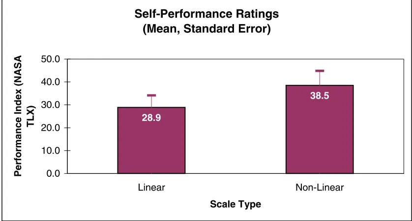
however, an inspection of the mean values for Performance seemed to indicate a slight
trend towards less confidence in performance level in the non-linear scale types. In fact,
when grouped according to major scale types (linear versus non-linear), the ANOVA
yielded a significant difference in the Performance ratings, F(1,82) = 18.65, p < .0001,
scale types was 38.5 (Figure 3.12). Although this secondary grouping and analysis may
be viewed as a re-use of data, and hence raising the family-wise type I error, the
computed alpha level is small enough to eliminate any concerns of falsely rejecting the
null hypothesis.
Self-Performance Ratings (Mean, Standard Error)
28.9
38.5
0.0 10.0 20.0 30.0 40.0 50.0
Linear Non-Linear
Scale Type
Performance Index (NASA
TLX)
Figure 3.12. Mean performance ratings for mileage estimation task (note that lower numbers constitute higher satisfaction with performance).
3.2.4 Individual Differences
A multi-correlational analysis was performed between each of the dependent
variables and the participants’ gender, subjective ratings of mathematical ability (MA)
and spatial reasoning (SR), and map experience. Results of this analysis indicated no
significant correlations between either of the subjective abilities and response accuracy
and response time. However, a significant correlation was obtained between MA and the
TLX Mental Demand index, r = -.21, p < .05. The interpretation of these correlations is
provided in the discussion below. No gender differences were found.
3.3 Experiment I Discussion
Results of Experiment I indicate that the combination of more than one scale
along a horizontal axis does not have a statistically significant effect on mileage
estimation accuracy. Accuracy, however, was affected by the distance between target
pairs as illustrated in Figure 3.7. In particular, error increased as the distance between
target pairs increased. This finding supports what would be expected due to Weber’s
Law, that errors increase as a constant percentage of the actual stimulus intensity or
dimensions. In this case, the errors were generally between 11-13% of the inter-target
distance.
It was found that response time increased as additional scales were included along
the grid. In particular, the significant differences were found between the Half-Inch
Linear scale with both the Modified Fisheye and True Half-Inch Bifocal scale types (the
longest response times belonging to the Modified Fisheye and the ½” True Bifocal scales,
the shortest to the ½” Linear scale). This increase was expected since with the addition
of scales comes the necessity to perform additional mental calculations before an answer
can be formulated. Furthermore, a response time increase might be expected given the
pure novelty of the non-linear treatment conditions. It is quite possible that the
magnitude of the increase would diminish with additional exposure to the non-linear
conditions.
The distance between the individual target pairs was also found to affect the
increase as the distance between targets increased (which is also supported by the
significant correlation). The significant interaction between Scale Type and Target Pair,
as shown in Figures 3.10 and 3.11, reveals that response times increased for all display
types with increasing distance between targets, but the increase was more abrupt for the
non-linear than the linear scale types. This, again, can be attributed to the need to
combine more than one scale in the estimation process, thereby amplifying the general
trend seen in Figure 3.9.
Overall Workload was not affected by the addition of scales. This finding may be
due to the relative simplicity of the task itself, since it was a simple perception study with
no experimentally-imposed time restrictions. While the individual workload index,
Performance, did not differ significantly when the scale types were examined
individually, an examination in which linear and non-linear scale types were grouped in
kind, shows that the participants in the non-linear conditions felt less confident/satisfied
in their performance level than those in the linear conditions. This confidence difference
exists in spite of the fact that the actual performance level (i.e., accuracy) was not
significantly different between major scale types. Again, this is most likely due to the
novelty of the non-linear stimuli. It is suggested that satisfaction levels would likely
increase as individuals become more accustomed to working with multiple scale grids.
Results in the examination of the individual difference data indicate a negative
correlation between the participants’ subjective mathematical and spatial reasoning
ability level with their satisfaction/confidence in task performance. The negative
individual with their mathematical and spatial reasoning abilities, the more confident they
were in their performance level (regardless of what the accuracy and response time data
actually showed). Based on the significant correlation between map use and the Mental
Demand index, participants who claimed to have experience with maps (for other than
driving purposes) seemed to think the task was less mentally demanding than those with
no map experience, but again, there was no significant relationship with their actual
performance level. The lack of significant correlations between the individual
differences and performance data may be due, at least in part, to unreliable subjective
aptitude ratings.
The results of this experiment indicate no significant detriment in mileage
estimation accuracy, but an increase in estimation response time when using multiple
scale maps. This task, however, was limited to a one-dimensional estimate along a
horizontal axis. The next obvious step, then, is to determine if these findings are
isotropic. That is, are people as accurate at estimating distances at various stimulus
orientations? How are response times affected by target orientation? The issue of angle
estimation must also be addressed since this is the other principle navigation task for
which maps are used. Furthermore, as discussed in the literature review, various types of
distortions can be applied to map images. Which distortion type is best suited to these
4. EXPERIMENT II: THE EFFECT OF DISTORTION TYPE ON MILEAGE AND HEADING ESTIMATION
The purpose of this experiment was to determine if one of two distortion types,
Cartesian or polar, is better suited to navigation performance than the other, and to
validate the performance findings from Experiment I in a two-dimensional domain.
Performance in heading estimation was added to the basic paradigm followed in the
Experiment I method. The specific hypotheses addressed are:
Hypothesis 1: Mileage estimation accuracy will decrease when viewing targets on a distorted grid-type.
Hypothesis 2: Response time during mileage estimation will increase when viewing targets on a distorted grid-type.
Hypothesis 3: Heading accuracy will decrease when viewing targets on a distorted grid-type.
Hypothesis 4: Response time during heading estimation will increase when viewing targets on a distorted grid-type.
Hypothesis 5: Perceived workload will increase when targets are viewed on a distorted grid-type.
4.1 Method
4.1.1 Subjects
Forty-eight individuals (23 men and 25 women) participated in this study. Of the
forty-eight, forty-two were students enrolled in a variety of undergraduate and graduate
disciplines at North Carolina A&T State University, while the remaining six were staff
old. All subjects were paid ten dollars upon their completion of the experiment, and
some students were given extra credit by course instructors for participation in the
experiment.
4.1.2 Apparatus
As in the first experiment, the software for this experiment was created using
Rapid. All stimuli were presented on a 17” diagonal monitor set to a resolution of 1024
x 768 pixels and 24 bit colors, while the CPU contained a 400 MHz PentiumII
processor. The software collected performance data (accuracy and response times) online
during the experimental trials.
4.1.3 Experimental Design
A between subjects design was again chosen to control for possible asymmetrical
transfer of learning effects. As in Experiment I, subjects were assigned to one of three
experimental conditions based on the order in which they arrived for testing. The
independent variables for this experiment were Distortion Type, which contained three
levels: Linear (L), Cartesian Bifocal Distortion (CBD) and Modified Fisheye Distortion
(MFD), and Target Pair (representing 32 different angle/distance combinations about the
X-Y axes). Dependent variables were Mean Absolute Error (for mileage and heading
estimates), Response Time (for mileage and heading estimates), the TLX measure of
Overall Workload, as well as the TLX individual workload indices of Mental Demand,
4.1.4 Stimuli
There were three different “map” backgrounds used in this experiment, one for
each experimental condition. The Linear condition map (used by the control group) was
a 640 x 480 pixel rectangular grid subdivided into 80 x 80 pixel squares (Figure 4.1). A
red square, meant to outline a military area of operation (AOR), was drawn in the middle
of the grid. As in Experiment I, the targets were red crosshairs centered on ¼” diameter
white circles. One target was always displayed in the center of the grid, while the second
was located at one of thirty-two locations dispersed evenly around the grid.
created to distort any bitmap image into either a bifocal or modified fisheye distorted
bitmap image. After prompting for the input file, the software asks the user to input the
proportion of the image center to remain linear, as well as the scale multiplier to apply to
the peripheral data points. For both the CBD and MFD images, the input parameters
were set to a 0.46 linear center and a 0.5 scale multiplier. This resulted in a CBD image
size of 400 x 320 pixels (Figure 4.2), and a MFD image size of 432 x 352 pixels (Figure
4.3). The linear center proportion was selected such that the center four grid locations
would remain completely linear. The scale multiplier was chosen due to the stronger
performance of participants in the True Half-Inch Bifocal condition over those in the
Quarter-Inch Bifocal condition of Experiment I.
Figure 4.3. Distorted stimulus employed for the Modified Fisheye treatment group.
The map scale used as the basis for mileage estimations was provided to the right
of the grids. Because of the uniqueness of the non-linear conditions (i.e., the
representation of scale changes across the grids) the scale was modified to show grid
subsection dimensions as opposed to a combination of standard one-dimensional scales.
It was thought that the rectangular scale would be easy to understand since the grid
subsections always represent the same area (four square miles, in this case) regardless of
4.1.5 Procedure
Upon reporting for the experiment, participants were briefed regarding the
purpose and basic procedures of the study, and were then asked to sign a consent form.
As in Experiment I, demographic data collected included age, gender and field of study.
Participants were also asked to subjectively rate their mathematical and spatial reasoning
abilities on a five-point Likert scale, and to indicate whether they had previous
experience using maps (for other than driving purposes). Each participant’s vision was
tested using a standard Snellen visual acuity chart. Only those individuals with 30/20 or
better vision (with or without corrective lenses) were allowed to proceed to the training
phase. Only one individual was turned away for insufficient visual acuity.
4.1.5.1 Training
Because the task of angle estimation is not as common or elementary as distance
estimation, it was desired to train each subject to estimate angles to a certain degree of
proficiency before commencing with the experimental trials. Therefore, a
computer-based training device (Figure 4.4) was developed. This device trained individuals to
estimate twelve different angles, each a multiple of 22.5 degrees, and did not include
those that fall on the cardinal axes themselves. These specific angles were chosen
because of the varying magnitude of the non-linear distortion effects that can occur at
various angular locations about the axes, specifically in the Cartesian Bifocal distortion.
Trainees were instructed to use the slider switch to adjust the pointer’s position
about the axes until they thought it reflected the presented target angle. When satisfied
actual angle. The error in degrees was also provided in alphanumeric format as
additional feedback. After viewing the error information, the “Next” button was
depressed, and another target angle was presented. Once each of the twelve angles had
been estimated, the absolute median error was computed and displayed to the trainee.
Each participant repeated the training program five times before proceeding to the data
collection phase (an earlier pilot study of 17 individuals indicated that the learning curve
appeared to flatten out following five training trials). The median absolute errors over
the five trials were then averaged, and this value was recorded for inclusion in data
analysis.
4.1.5.2 Data Collection
Following the training phase, the experimenter demonstrated the software for the
subjects and explained the actual task to be performed. Subjects were then given time to
familiarize themselves with the apparatus before the start of data collection, and were
positioned at a “normal” viewing distance (about 24 inches) from the monitor.
Participants were instructed that accuracy was most important, but to work quickly as
well. Once the individual was satisfied with their understanding of the task, the
experimental trial was initiated.
At the start of the task, the grid and mileage scale was presented on the computer
monitor, where they remained throughout data collection. Following a five-second
waiting period, a randomly selected set of two targets appeared on the grid. Subjects
were first queried to estimate the mileage between target centers, and key in their
estimate using the keyboard. Response times were recorded as the time lapse between
target presentation (and the simultaneous query statement) and the moment the first key
was pressed. When the “Enter” key was pressed, the subjects were immediately queried
to estimate the heading (i.e., the angle) between the same target pair. Query statements
were accompanied by the presentation of a short tone to assist in alerting the subject.
Response time was again recorded as the time lapse between the appearance of the query
statement and the time the first key was pressed. Once the heading estimate was entered,
the targets disappeared, and a five-second inter-stimulus timer began. A new set of
targets was presented following each inter-stimulus break.
Thirty-two different target pairs were presented throughout each trial. Two