ABSTRACT
DEVINENI, NARESH. Multimodel Ensembles of Streamflow Forecasts: Role of Predictor State in Developing Optimal Combination. (Under the direction of Sankar Arumugam.)
MULTIMODEL ENSEMBLES OF STREAMFLOW FORECASTS: ROLE OF PREDICTOR STATE IN DEVELOPING OPTIMAL COMBINATION
by
NARESH DEVINENI
A thesis submitted to the Graduate Faculty of North Carolina State University
in partial fulfillment of the requirements for the Degree of
Master of Science
CIVIL ENGINEERING Raleigh, North Carolina
2007
APPROVED BY:
Dr. S. Ranji Ranjithan Dr. E. Downey Brill
DEDICATION
BIOGRAPHY
ACKNOWLEDGEMENTS
I would like to express my profound sense gratitude to Dr. Arumugam for being an excellent mentor and for providing me with necessary guidance and support at every step of my Masters study. I am deeply indebted to him for transforming me not only into a complete engineer but also as a responsible person. I am grateful to Dr. Ranjithan who has given feed back from time to time on my performance and boosted my morale and confidence under difficult situations. I would also like to thank Dr. Downey Brill for his encouraging words on my performance. I am very honored to work under the guidance of these people.
I am always grateful to my parents and grand parents, with whose constant support, encouragement and blessings I was able to come to the United States to pursue my higher degree. I also thank my brother Ravi Chandra Devineni for his constant belief in me and my capabilities as a performer.
I thank Mr. Kurt Golembesky for his valuable feed back and discussions on my thesis. I would like to thank my friends Shravan Chintapatla, Krishi Siravuri and Uday Maripalli for helping me out in difficult situation. A special thanks to Pawan Imanneni with whose guidance I could make it to NC State University. I would like to thank my friends Praveen Gollakota, Sarat Sreepathi, Sridevi Chalasani, Azam Hossain, Jitendra Kumar and Mr.Satish Regonda for their help, support and feedback.
TABLE OF CONTENTS
LIST OF TABLES………...vii
LIST OF FIGURES………viii
1 Introduction……… ………...1
1.1 Multi-Year Drought and Falls Lake Management….………1
1.2 Climate Forecasting and Water Supply Management………...3
1.3 Streamflow Forecasts – Development Methodologies….………...……..4
1.4 Improvement of Multi Model Streamflow Forecasts……..………...5
1.5 Outline of the Thesis………..………....7
2 Literature Review………..…………...8
2.1 Sea Surface Temperature (SST) –Streamflow Teleconnection…….…….…...8
2.2 Model uncertainty and Multi-Model combination methods………....10
3 Seasonal Streamflow Forecasts Development for the Falls Lake………...….14
3.1 Hydroclimatology of Neuse Basin……….….….14
3.2 Seasonal Streamflow Forecasts Development – Individual Models………....15
3.3 Predictor Identification………..……….….16
3.4 Dimension Reduction-Principal Component Analyses on SSTs.…….…..….17
3.5 Performance of Individual Models...20
4 Multi-Model Ensembling Based on Predictor State: Methodology Development..…25
4.1 Motivation………...…….…25
5 Multimodel Ensembles of Streamflow forecasts for the Falls Lake…..…………...33
5.1 Skill of Individual Models from Predictor state space……….…34
5.2 Performance of Multi-Model Forecasts………...…36
5.3 Role of Multi-Model Forecasts in improving the forecast reliability...40
6 Multimodel Climate Forecasts for the US………...44
6.1 General Circulation Models and their role in climate prediction……….…...44
6.2 Source of uncertainty in model prediction………...46
6.3 Multi-Model Ensembles of GCMs: Motivation…..……….47
6.4 Multimodel winter precipitation forecasts for the US……….50
6.5 Results and Analysis………....51
7 Summary and Conclusions………..…55
7.1 Streamflow forecasts for the Falls Lake……….……….…55
7.2 Precipitation Forecasts for the US……….………..57
7.3 Future Work……….…57
7.4 Publications……….…….58
8 References……….………..….59
9 Appendix ...………..………....69
LIST OF TABLES
Table 3.1 Performance of individual models forecasts under leave-1 out cross validated forecasts and adaptive
forecasts………...………23 Table 5.1 Performance of individual model forecasts and various
multi-model schemes under leave-1 out cross validated forecasts and adaptive forecasts for two different
LIST OF FIGURES
Figure 1.1 Recent multi-year drought conditions in NC……….…2
Figure 1.2 Location of Falls Lake Reservoir in Raleigh NC……… …...3
Figure 3.1 Seasonality of Neuse River Basin………....15
Figure 3.2 Predictor Identification………18
Figure 3.3 Scree plot of Principal components of SSTs………...21
Figure 3.4 Performance of individual models………...24
Figure 4.1 Importance of assessing the skill of the model from predictor space………..27
Figure 4.2 Flowchart of the multi-model ensembling algorithm……….…….32
Figure 5.1 Performance of individual models from the predictor state space……...36
Figure 5.2 Performance of multi-model forecasts……….…………...39
Figure 5.3 Relationship in choosing different neighbors……….….40
Figure 5.4 Reliability of models for below normal and above normal conditions……....43
Figure 6.1 Predictability of two GCMs over the US for different climate states……..…49
Figure 6.2 Skill of individual models and the combined multi-model……..……..……..53
Figure 6.3 Performance of CCMv6 under the causal relation of SST with observed precipitation……….…...………..54
Figure A-1 Observed Category falling in Below Normal……….……….72
Figure A-2 Observed Category falling in Normal……….……….73
CHAPTER 1
INTRODUCTION
Information on season-ahead streamflow forecasts is beneficial for operation and management of water supply systems and in addressing the issues of droughts and floods. Unless closely monitored using various sector-specific indicators, the impacts of droughts and floods are progressive, persistent and pervasive over a larger area. Prediction of these hydroclimatic extremes well in advance would help local/state water managers and emergency management agencies to develop appropriate contingency measures and alternative water management strategies. For instance, long-lead (3 months to 6 months ahead) prediction of drought will provide vital information in hedging the associated risk as well as in imposing voluntary restrictions for water supply systems.
1.1 Multi Year Drought and Falls Lake Management
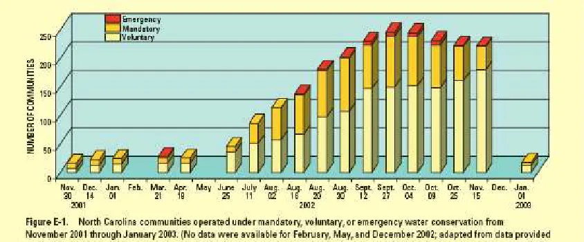
figure 1.1, the severity of droughts is more pronounced during summer months (July – August – September).
Figure 1.1: Recent multi-year drought conditions in NC. Figure shows the number of communities in North Carolina that were under voluntary, mandatory and emergency restrictions from 2001-2003 [Yonts W, 2004].
Figure 1.2: Location of the Falls Lake Reservoir in Raleigh NC.
1.2 Climate Forecasting and Water Supply Management
1.3 Streamflow Forecasts- Development Methodologies
1.4 Importance of Multi Model Streamflow Forecasts
1.5 Outline of the Thesis
CHAPTER 2
LITERATURE REVIEW
Hydroclimatic extremes like droughts and floods are generally associated with low frequency climate fluctuations like El Niño Southern Oscillations (ENSO) and decadal and interdecadal climatic modes such as Pacific Decadal Oscillation (PDO) and North Atlantic Oscillation (NAO). ENSO is a quasi oscillatory mode of coupled ocean atmosphere interactions in the tropical Pacific with a characteristic narrow band width of 2 to 7 years. These climate modes govern the interannual variability of climate over most of North America. The following section details the work done in understanding these climatic modes and its teleconnection to the climate variables like precipitation and streamflows.
2.1 Sea Surface Temperature (SST) – Streamflow Teleconnection
Ocean primarily determine the interannual variability in precipitation over North and South America [Rasmusson and Carpenter 1982, Ropeleweski and Halpert, 1987]. Studies have shown that ENSO conditions also influence anomalous SST conditions in the tropical Atlantic and Indian Ocean, hence affecting global climate [Enfield 1989]. There are also other dominant decadal and interdecadal climatic modes such as Pacific Decadal Oscillations (PDO) and North Atlantic Oscillations (NOA) that putatively govern the interannual variability in climate over North America [Sankarasubramanian and Lall, 2003].
ENSO-related teleconnection between precipitation and temperature during both winter and summer seasons over NC [Roswintiarti et al., 1998; Rhome et al., 2000].
Thus, associating seasonal to interannual variations in streamflow variability with low frequency climatic variability will provide useful information in developing season ahead streamflow forecasts contingent on climatic conditions. In this study, we develop season ahead streamflow forecasts for the Falls Lake using two low dimensional models and then combine them to develop multi model ensembling streamflow forecasts for Falls Lake. The next section provides a brief background on multi model ensembling techniques that are currently pursued in the literature for developing operational climate and streamflow forecasts.
2.2 Model uncertainty and Multi-Model combination methods
partly arise from increase in the sample size, studies have compared the performance of single models having the same number of ensembles as the pooled multi-model ensembles and have shown that multi-model approach naturally offers better predictability because of the ability to incorporate outcomes from multiple models, thereby encompassing underlying different process parameterizations and schemes [Hagedorn et al., 2005]. Since the advantage gained through multi-model ensembling is a better representation of conditional distribution of climatic attributes, it is important to evaluate probabilistic forecasts developed from multi-model ensembles through various performance evaluation measures and by analyzing the predictability for various geographic regions [Doblas-Reyes et al., 2005]. Recent studies have also considered climatology as one of the forecasts in developing multi-model ensembles [Rajagopalan et al., 2002; Robertson et al., 2004].
employ statistical methods such as linear regression has also been employed so that the developed multi-model forecasts has better skill than single models [Krishnamurthi et al., 1999]. However, application of optimal combination approach using either statistical or optimization techniques require observed climatic or streamflow attributes at a particular grid point or station. Studies have also used advanced statistical techniques such as canonical variate method [Mason and Mimmack, 2002] and Bayesian hierarchical method [Stephenson et al., 2005] for developing multi-model combinations. Hoeting et al., [1999] show that the mean of the posterior distribution of the predictand obtained by averaging over all the models with its probability of occurrence provides better predictive ability (measured by logarithmic scoring rule) than the mean of the posterior distribution of the predictand obtained from a single model.
CHAPTER 3
SEASONAL STREAMFLOW FORECASTS DEVELOPMENT FOR THE
FALLS LAKE
Development of probabilistic seasonal streamflow forecasts from two different models based on climate information for the Falls Lake, Neuse river basin in North Carolina (NC) is the first objective of this study. Streamflow forecasts based on two low dimensional statistical models, one based on parametric regression approach and another using a nonparametric approach based on resampling [Souza and Lall, 2003] were developed. A brief baseline information about the Neuse basin and its importance to the water management of the research triangle area of NC is provided in the next section.
3.1 Hydroclimatology of Neuse Basin
forecasting models for the low flow season is important since maintaining the operational rule curve of 251.5’ is challenging during those months.
0 200 400 600 800 1000 1200 1400 1600 1800 2000 J a n F e b M a r A p r M a y J u n e J u ly A u g S e p O c t N o v D e c Months S tr e a m fl o w (f t 3 /s ) average 25th percentile 75th percentile
Low Flow Season JAS - 14% High flow season
JFM - 46%
Figure 3.1: Seasonality of Neuse River Basin
3.2 Seasonal Streamflow Forecasts Development – Individual Models
The key objective is to estimate the conditional distribution of streamflows, f(Qt|Xt),
that would occur in the upcoming season based on the climatic conditions Xt using the
chosen statistical model. The estimate of the conditional distribution of streamflow forecasts
is m t i
Q, with‘t’ denoting the time, ‘i’ representing the ensemble and ‘m’ denoting the model.
could be estimated through a parametric approach which explicitly specifies a functional form (e.g., log normal) for the conditional distribution. The other method is to use a data driven approach which estimates the conditional distribution by using nonparametric techniques such as resampling. For the parametric approach, a regression model by assuming the flows follow a lognormal distribution is employed. The estimate of the conditional mean and standard deviation of the lognormal parameters are obtained from the regression estimate and from the point forecast error respectively, which is computed based on the variance of the residuals. Using the lognormal parameters of conditional mean and conditional standard deviation, ensembles from lognormal distribution are generated and are transformed back
into the original space to represent the conditional distribution of flows, m t i
Q, . The other
approach is the semi-parametric resampling algorithm reported by Souza and Lall [2003]. The main advantage of this approach is that it does not specify any functional form for estimating the conditional distribution, thus allowing the data to describe the conditional distribution by considering climatic conditions that are similar to current conditions.
3.3 Predictor Identification
predictors that influence the streamflow into Falls Lake during JAS, SST conditions during April-June (AMJ) which could be obtained from IRI data library were considered.
(http://iridl.ldeo.columbia.edu/expert/ SOURCES/.KAPLAN/.EXTENDED/.ssta).
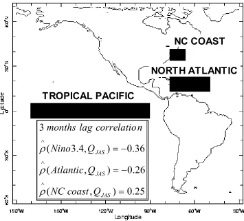
Predictors are identified using Spearman rank correlation measures which are more powerful in detecting non-linear dependencies between the predictor and the predictand. Figure 3.2 shows the spearman rank correlation between the observed streamflow during JAS at the Falls Lake and the SST conditions during AMJ. From the figure 3.2, we see clearly that SST over ENSO region (170E - 90W and 5S - 5N), the North Atlantic region (80W- 40W and 10N - 20N), and the NC Coast region (75W- 65W and 22.5N- 32.5N) influence the summer flows into Falls Lake. An important note is that SST regions whose correlations are
significant and greater than the threshold value of ±1.96/ n−3 where ‘n’ is to the total number years (n=75 years for Falls Lake) of observed records used for computing the correlation were considered. Figure 3.2 also shows the 3 month lag correlation between the identified predictors and the streamflow at the Falls Lake reservoir. The negative correlation indicated in figure 3.2 suggests that above normal conditions in the Sea Surface Temperature in the tropical Pacific will influence below normal conditions in the Falls Lake and vice versa.
3.4 Dimension Reduction – Principal Component Analyses on SSTs
Figure 3.2: Predictor Identification. Figure shows the SST regions that influence the streamflow into the Falls Lake. SST regions that has significant correlation at 95% confidence interval (> 0.22 or < -0.22) are only considered for model development. Also shown in the figure is the 3 month lag correlation of the identified predictors and the streamflows at the Falls Lake.
Principal Components Analysis (PCA) is a multivariate procedure which rotates the data such that maximum variability is projected onto the axes. Essentially, a set of correlated variables are transformed into a set of uncorrelated variables which are ordered by reducing the variability. The uncorrelated variables are linear combinations of the original variables, and the last of these variables can be removed with minimum loss of real data. The first
principal component is the combination of variables that explains the greatest amount of variation in the original predictor. The second principal component defines the next largest amount of variation that is remaining and is independent to the first principal component. There can be as many possible principal components as there are variables. In general the mth principal component is the weighted linear combination of the X’s or the predictor data set.
Principal component analysis generally gives three outputs, principal components (scores), Eigen vectors (loadings), Eigen values (% variance explained). The first few components explain most of the variance of the original data. The first few eigenvectors will point in the directions where the data jointly exhibits large variations. The remaining eigenvectors will point to directions where the data jointly exhibits less variation. For this reason, it is often possible to capture most of the variation by considering only the first few eigenvectors. The Eigen vectors are useful to locate the source of variability. The variance of the mth principal component is the mth eigenvalue. Therefore, the total variation exhibited by the data is equal to the sum of all eigenvalues. The Eigen values are useful to choose the dominant principal components. A Scree Plot is a simple line segment plot that shows the fraction of total variance in the data as explained by each component. Mathematics of PCA and the issues in selecting the number of principal components using scree plot could be found in Dillon and Goldestein [1984], Wilks [1995] and Von storch and Zweiers [1998].
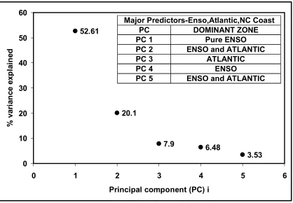
performed by singular value decomposition (SVD) on the correlation matrix or covariance matrix of the predictors. Since PCA is scale dependent, loadings (Eigen vectors or EOF patterns) obtained from covariance matrix and correlation matrix are different. Importance of each principal component is quantified by the fraction of the variance the principal component represents with reference to the original predictor variance, which is usually summarized by the scree plot. Figure 3.3 shows the percentage of variance explained by each principal component, and the first two components account for 72% of the total variance shown in the predictor field in Figure 3.2. Based on the eigenvectors obtained from PCA, the first component representing the ENSO region has correlation of 0.36 with observed streamflow and the second component representing the Atlantic has a correlation of -0.23 (significance level +/- 0.22 for 75 years of record) with the inflows at Falls Lake. We employ these two principal components to develop seasonal streamflow forecasts for JAS for the Falls Lake.
3.5 Performance of Individual Models
Figure 3.3: Scree plot of the principal components of the SSTs in the three regions (in Figure 3.2) indicating the % variance explained by each component. The dominant zone of each PC obtained based on eigen vectors of the PC is also indicated.
By utilizing the two principal components from PCA, both leave-one-out cross validated retrospective streamflow forecasts and adaptive streamflow forecasts for the season JAS are developed using the two mentioned statistical models. Leave-one-out cross validation is a rigorous model validation procedure that is carried out by leaving out the predictand and predictors from the observed data set (Qt, Xt, t =1, 2, n) for the validating year
and the model is developed using the rest of the (n-1) observations. For instance, to develop retrospective leave-one-out forecasts from parametric regression, a total of ‘n’ regression models are developed by leaving out the observation in each validating year. By employing
52.61 20.1 7.9 6.48 3.53 0 10 20 30 40 50 60
0 1 2 3 4 5 6
Principal component (PC) i
% v a ri a n c e e x p la in e
d ENSO and ATLANTIC
ATLANTIC ENSO
ENSO and ATLANTIC PC 2
PC 3 PC 4 PC 5
Major Predictors-Enso,Atlantic,NC Coast
PC DOMINANT ZONE
the developed forecasting model with (n-1) observations, the left out observation (Q-t, with -t
denoting the left out year or the validating year) is predicted by using the state of the predictor/principal components (X-t,) in the validating year. To obtain adaptive streamflow
forecasts, we develop the forecasting models based on the observed streamflow and the two dominant principal components from 1928-1987 and employ the developed model to predict the streamflow for a 15 years period from 1988-2002.
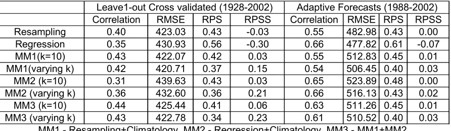
Table 3.1: Performance of individual models forecasts under leave-one-out cross validated forecasts and adaptive forecasts. The performance evaluation measures are calculated based on 75 years of data for leave-one-out cross validated forecasts and 15 years for adaptive forecasts from 1987-2002.
Correlation RMSE RPS RPSS Correlation RMSE RPS RPSS Resampling 0.40 423.03 0.43 -0.03 0.55 482.98 0.43 0.00 Regression 0.35 430.93 0.56 -0.30 0.66 477.82 0.61 -0.07
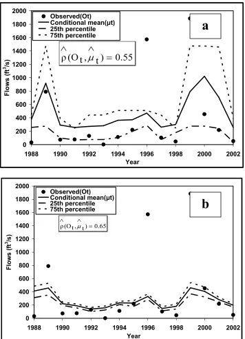
0 200 400 600 800 1000 1200 1400 1600 1800 2000
1988 1990 1992 1994 1996 1998 2000 2002
Year F lo w s ( ft 3 /s ) Observed(Ot) Conditional mean(µt) 25th percentile 75th percentile
0.55
)
t
,
t
(O
ρ
=
∧
∧
µ
0 200 400 600 800 1000 1200 1400 1600 1800 20001988 1990 1992 1994 1996 1998 2000 2002
Year F lo w s ( ft 3 /s ) Observed(Ot) Conditional mean(µt) 25th percentile 75th percentile 0.65 ) t , t (O ρ = ∧ ∧ µ
Figure 3.4: Performance of individual models in predicting observed streamflows during 1988-2002 for the Falls Lake. 3.4(a) Semi-parametric resampling model of De Souza and Lall [2003] 4(b) parametric regression. Forecasts from both the models were obtained by using the observed streamflows during JAS and predictors (PC1 and PC2 in figure 3.3) for the period 1928-1987.
a
CHAPTER 4
MULTI-MODEL ENSEMBLING BASED ON PREDICTOR STATE:
METHODOLOGY DEVELOPMENT
Error resulting from climate forecasts is primarily of two types: (a) Uncertainty in initial and boundary conditions and (b) Model error [Hagedorn et al., 2005]. The first source of error is typically resolved by representing the uncertainties in initial and boundary conditions in the form of ensembles. The second source of error arises from process representation, which could be reduced by combining forecasts from multiple models which incorporate various process representation and model physics to develop an array of possible scenarios of outcomes. Developing multi-model ensembles combines these two strategies resulting in reducing both sources of error. However, even after developing multi-model ensembles could result with observations occurring outside the realm of these models (see Figure 8 in Hagedorn et al., 2005). Similarly, the performance of individual models and multi-model ensembles may be poor during certain boundary/SST conditions owing to limited relationship between SST conditions and precipitation/temperature over a particular location/grid [Goddard et al., 2003]. Under these climatic conditions with all models having poor predictability, it may be useful to consider climatology as a forecast.
4.1 Motivation
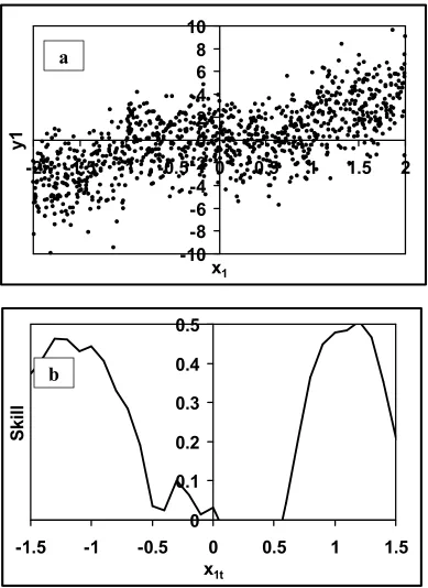
predictors, Xt =(x1t,x2t)with x1 influencing the predictand only if the absolute value of the predictor x1 is greater than the threshold value of 1. The underlying model is yt = 2x1t+0.5x2t
+εt if |x1t| > 1 and y1t = 0.25x2t +εt if |x1t| ≤ 1. The noise term εt follows i.i.d with a normal
distribution having zero mean and a standard deviation of 2. The predictors follow uniform distribution between -2 to 2. A total of n = 1000 realization is generated from this mixture model setup which could be analogously compared to two predictors as anomalous SST conditions influencing the local hydroclimatology. The correlation between y and x1 is 0.671
and y and x2 is 0.134, which would suggest one to give higher importance to predictor x1.
Figure 4.1b shows the skill (correlation) of the fitted regression model between y and x1
against x1. To evaluate the correlation between y and the fitted values (y on x1) against x1, we
consider a bandwidth of 1 on x1 such that the fitted values of y obtained using the predictor
x1 within that bandwidth are only considered. Note the poor skill between predictand y and
the fitted values of y during x1t= -0.5 to 0.5.
-10
-8
-6
-4
-2
0
2
4
6
8
10
-2
-1.5
-1
-0.5
0
0.5
1
1.5
2
x
1y
1
0
0.1
0.2
0.3
0.4
0.5
-1.5
-1
-0.5
0
0.5
1
1.5
x
1tS
k
il
l
Figure 4.1: Importance of assessing the skill of the model from the predictor space.
a
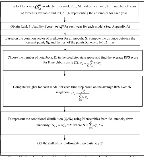
4.2 Multi-Model Ensembling based on Predictor State Space – Algorithm
Development
Let us suppose that we have streamflow forecasts, m t i
Q, , where m=1,2..,M denoting the
forecasts from ‘M’ different models, i = 1,2, ..N representing ensembles of the conditional distribution of streamflows with ‘N’ denoting the total number of ensembles under each model, and ‘t’ denoting the time (season/month) for which the forecast is issued. Assuming that we have a total of t= 1,2,...n years for which the forecasts, m
t i
Q, , are available and the
models also have a common predictor vector, Xt, which influences the conditional
distribution of hydroclimatic attributes represented using the ensembles. Figure 4.2 provides a flow chart indicating the steps in implementing the proposed multi-model ensembling conditioned on the predictor state. It is important that the proposed approach requires at least one common predictor among the ‘M’ competing models. Even if the models do not have a common predictor particularly in the context of GCM forecasts, one could use the leading principal component of the underlying boundary conditions (for instance, SSTs) as the common predictor across all the models. As mentioned before, developing multi-model ensembles based on optimal combination method requires the observed climatic/streamflow variables Ot, using which one could assess the skill of the probabilistic forecasts using Rank
Probability Score (RPS) [Murphy 1970, Candille and Talagrand 2005, Anderson, 1996] to obtain the weights wtm. It is important to note that RPS is evaluated each year using the
reference forecast strategy which is usually assumed to be climatology. Appendix A provides details on obtaining RPS and RPSS for a given probabilistic forecasts.
Let us denote the RPS and RPSS of the probabilistic forecasts, m t i
Q, , for each time step
as m
t
RPS and m
t
RPSS ,respectively. Our approach to assess the skill of the model is its ability
to predict under similar climatic conditions or the predictor state, which could be identified by choosing a distance metric that computes the distance between the current predictor state,
Xt,and the historical predictor vector, X. One could use simple Euclidean distance or a more
generalized distance measure such as Mahalonobis distance metric, which is more useful if the predictors’ exhibit correlation among them. Compute the distances dtl between the current
conditioning state Xt, and the historical predictor vector Xlas
) (
ˆ ) (
d 1 t l
T
l t
tl = X −X ∑ X −X
−
... (1)
where ∑ˆ denotes the variance-covariance matrix of the historical predictor vector X. One can note that if l=t, the distance metric, dtl, reduces to zero. Using the distance vector d, the
ordered set of nearest neighbor indices J can be identified. Thus, the jth element in the distance vector metric provides the jth closest Xl to the current state Xt. Using this
information, we assess the performance of each model in the predictor state space as
∑
= = λ K j m j RPS K 1 ) ( m K t, 1 ... (2)where RPS(j) denotes the skill of the forecasting model for the year that represents the jth
closest condition (obtained from J) to the current condition Xt. In other words, λmt,K
summarizes the average skill of the forecasting model, m, by choosing ‘K’ years that
each time step, we obtain the weights for multi-model ensembling so that the models with better performance during a particular climatic conditions needs to be represented with more number of ensembles in comparison to a model with lower predictability under those conditions. It is important to note that RPS is a measure of error in predicting the probabilities and it is evaluated based on the entire ensembles that represent the conditional distribution of streamflows.
∑
= λ λ = M m m K t m K t m K t w 1 , , , / 1 / 1 ... (3)If λmt,K is zero for a subset of models M1≤ M, then the weights wtm,K are distributed
equally between the models for which λmt,K is zero with the rest of models’ weights being
equal to zero. The multi-model forecasts for each time step could be developed by drawing
N
wtm,K * ensembles from each model to constitute the multi-model ensembles. Thus, one has
to specify the number of neighbors ‘K’ to implement this approach. It is also important to note that choosing fewer ‘K’ relates to evaluating the model performance over few years of similar conditions, which does not imply that the forecasts are developed from the
predictands and predictors based on the identified similar conditions. In fact, m t i Q, are
Thus, we use the weights,wtm,K, only to draw the ensembles fromQim,t, which is in fact
developed based on the chosen training period in developing the forecasts. The simplest approach for selecting the number of neighbors is to find a fixed ‘K’ that provides improved predictability using multi-model ensembles over ‘n’ years of forecasts. We evaluate two different methods in choosing the number of neighbors ‘K’ to develop multi-model ensembles. The performance of multi-model ensembles is also compared with individual model’s predictability using various verification measures such as average RPS, average RPSS, anomaly correlation and root mean square error (RMSE). To apply the same algorithm for kt that gives the minimum RPS from the multi-model ensembles, compute
MM k t
RPS, for k=1, 2, n-1 and choose k that corresponds to minimum MM k t
RPS, . Thus, by computing
MM k t
RPS, for all the data points, we choose the number of neighbors, kt that has the
minimum MM k t
Figure 4.2: Flowchart of the multi-model ensembling algorithm described in section 4.2 for fixed number of neighbors ‘K’ in evaluating the model skill from the predictor state space.
Select forecasts,
m
t
i
Q
,
available from m=1, 2…, M models, with t=1, 2…n number of yearsof forecasts available and i=1,2…,N representing the ensembles for each year.
Obtain Rank Probability Score,
RPS
t
m
for each year for each model (See, Appendix A)Based on the common vector of predictors for all models, X, compute the distance between the current point, Xt, and the rest of the points Xl, where l=1, 2…, n
Choose the number of neighbors, K, in the predictor state space and find the average RPS score for K neighbors using (2):
∑
= = K j m j m k t RPS K 1 ) ( , 1 λ
Compute weights for each model for each time step based on the average RPS over ‘K’ neighbors
∑
= = M m m K t m K t m K t w 1 , , , 1 1 λ λTo represent the conditional distribution (Qt/Xt) using N ensembles from ‘M’ models, draw
randomly, Nt,m =wtm,K*N where N =
∑
= M m m K t N w 1 , *
CHAPTER 5
MULTIMODEL ENSEMBLES OF STREAMFLOW FORECASTS FOR
THE FALLS LAKE
In this chapter, we apply the multi-model ensembling algorithm discussed in section 4.2 to combine the forecasts from individual models along with climatological ensembles. The motivation in considering climatology as one of the candidates is upon the presumption that if the observation falls outside the scope of all the models under certain predictor conditions, then climatology should be preferred over individual model forecasts. Recent studies have also shown that a two step procedure of combining first each individual model forecasts separately with climatology and then combining the resulting ‘M’ combinations at the second step to develop the final, single multi-model ensembles [Robertson et al., 2003; Goddard et al., 2003]. Combining individual models with climatology at one step results with one model getting all the weight (equal to one) leaving the rest of the models’ weights to zero [Rajagopalan et al., 2002; Robertson et al., 2004]. We also perform a two step procedure in developing multi-model ensembles by first combining the probabilistic forecasts from resampling model (MM1 in Table 5.1) and regression model (MM2 in Table 5.1) separately with climatology and then the resulting forecasts from two combinations are combined to develop the final multi-model forecasts (MM3 in Table 5.1). Further, we also choose the number of neighbors K in equation (2) by two different methods to identify the relevant predictor conditions: (a) by selecting a fixed ‘K’ that corresponds to improved multimodel forecasts over the validating period, and (b) varying Kt each year such that the
selected ‘Kt’ corresponds to the minimum RPS that could be obtained from multi-model
procedure in developing semiparametric and nonparametric models [Sankarasubramanian and Lall, 2003]. By varying Kt, we plan to investigate the role of choosing different Kt in
developing multi-model ensembles and their relation to predictor conditions.
Table 5.1: Performance of individual model forecasts and various multi-model schemes under leave-one-out cross validated forecasts and adaptive forecasts for two different strategies of choosing the number of neighbors K (fixed K and varying Kt). All the
performance evaluation measures are calculated based on 75 years of data for leave-one-out cross validated forecasts and 15 years for the adaptive forecasts from 1987-2002.
Correlation RMSE RPS RPSS Correlation RMSE RPS RPSS Resampling 0.40 423.03 0.43 -0.03 0.55 482.98 0.43 0.00
Regression 0.35 430.93 0.56 -0.30 0.66 477.82 0.61 -0.07 MM1(k=10) 0.43 422.07 0.42 0.03 0.55 512.83 0.45 0.01 MM1(varying k) 0.42 420.71 0.37 0.15 0.54 506.45 0.40 0.03 MM2 (k=10) 0.31 439.63 0.43 0.03 0.65 523.89 0.48 0.00 MM2 (varying k) 0.36 432.60 0.36 0.21 0.66 516.13 0.43 0.02 MM3 (k=10) 0.44 425.44 0.41 0.06 0.63 511.26 0.45 0.01 MM3 (varying k) 0.43 422.78 0.34 0.23 0.61 510.52 0.40 0.03 Leave1-out Cross validated (1928-2002) Adaptive Forecasts (1988-2002)
MM1 - Resampling+Climatology MM2 - Regression+Climatology MM3 - MM1+MM2
5.1 Skill of Individual Models from Predictor state space
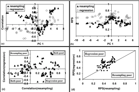
a fixed K = 10 based on the dominant predictor PC1. From figure 5.1a, one may prefer to choose forecasts from resampling model instead of forecasts from parametric regression particularly when the dominant principal component, PC1, is less than -2, since the predictive ability of regression model is negative during those conditions. This is seen in Figure 5.1b with the RPS of resampling being lesser than that of RPS of regression. Figures 5.1c and 5.1d show the relative performance of both models against each other. From figure 5.1c, we can see that one would prefer climatological ensembles particularly when correlations estimated from the neighborhood on both models are negative. From 5.1d, we can also identify conditions during which the RPS of regression model being higher than that of RPS of resampling. RPS is computed from the leave-one-out cross validated forecasts given in Table 5.1 for both candidate models and by assuming K=10 in equation (2). Correlation is computed between the observed streamflows and ensemble mean of the leave-one-out cross validated forecasts by considering 10 neighbors from the current state. Note the consistent poor performance of both the models in Figure 5c as well as for high negative values of PC1. Thus, the multi-model ensembling algorithm in section 4.2 identifies these conditions based on RPS using equation (2) and develops a general procedure for multi-model ensembling.
Figure 5.1: Performance of individual models from the predictor state space by considering K=10 neighbors: (5a) Correlation Vs PC1; (5b) RPSVs PC1; (5c) Correlation of regression Vs Correlation of resampling; (5d) RPS of regression Vs RPS of resampling.
5.2 Performance of Multi-Model Forecasts
As mentioned earlier, the multi-model combination is carried out in two steps: first combining individual model ensembles with climatological ensembles and then the resulting probabilistic forecasts from two combinations will be combined to develop final multi-model ensembles. To generate ensembles that represent climatology, we simply bootstrap the observed streamflows into Falls Lake assuming each year has equal probability of occurrence, which is a reasonable assumption given that there is no year to year correlation
-0.8 -0.6 -0.4 -0.2 0 0.2 0.4 0.6 0.8 1
-10 -8 -6 -4 -2 0 2 4 6 8
PC 1 C o rr e la ti o n resampling regression (a) 0 0.2 0.4 0.6 0.8 1
-10 -8 -6 -4 -2 0 2 4 6
PC 1 R P S resampling regression (b) 0 0.2 0.4 0.6 0.8 1
0 0.2 0.4 0.6 0.8 1
RPS(resampling) R P S (r e g re s s io n
) Regression poor
Resampling poor (d) -0.8 -0.6 -0.4 -0.2 0 0.2 0.4 0.6 0.8 1
-0.6 -0.4 -0.2 0 0.2 0.4 0.6 0.8 1
between the time series of summer flows. Figure 5.2a gives the multi-model adaptive forecasts by choosing a fixed K=10 in equation (2) for identifying similar conditions in the predictor state space. The fixed number of neighbors K=10 is chosen since it provided the lowest average RPS from multi-model ensembles for the period over which the forecast is developed. For leave-one-out cross validated forecasts, the average RPS is computed from 74 years of forecasts; For adaptive forecasts, average RPS is computed from 15 years of forecasts from 1988-2002. Thus, we chose the fixed ‘K’ by plotting the average RPS obtained for each neighbor from K = 1 to the maximum of the data length used for model fitting (for leave-one-out cross validated forecasts, it is 74 years; for adaptive forecasts, the maximum K = 60 years of record from 1928-1987) and choosing the value of ‘K’ that produced the lowest average RPS. Figure 5.2b provides adaptive forecasts developed from multi-model ensembles by choosing a varying Kt each year such that the chosen Kt for that
year corresponds to the minimum RPS that could be obtained from multi-model ensembles. By choosing K using any of the above strategy (fixed K or varying Kt), we assess the skill of
each year. Under varying Kt, the algorithm in section (4.2) is applied for 1≤ Κ≤ 60 t K (60
years of training data from 1928-1987) and Kt that corresponds to minimum RPS of the
multi-model ensembles is chosen for each year. Both figure 5.2 and Table 5.1 show very clearly that both strategies of choosing the number of neighbors result in significant improvements in predictability from multi-model ensembles compared to the probabilistic forecasts from individual models. It is important to note that the improved performance of multi-model ensembles is seen in almost all evaluation measures.
Even with fixed number of neighbors, the multi-model ensembling algorithm based on predictor state space provides improved predictability than the individual model forecasts. Ideally, one would like to have the number of neighbors varying each year so that the chosen Kt relates to the conditioning predictor state. For instance, under very high values of |PC1|,
very few years could be chosen as similar to the conditioning state. To understand whether we see any relationship between the chosen Kt for every year that corresponds to the
minimum RPS of the multi-model ensembles for that year, we plot the varying Kt with PC1
in figure 5.3. From figure 5.3, we see in general that smaller number of neighbors is chosen particularly if the PC1 corresponds to above normal or below normal values. Figure 5.3 also shows the distance between the conditioning state, PC1t and the chosen Kt in the predictor
PC1 space. It is important to note that PC1 primarily denotes ENSO conditions (correlation between PC1 and Nino3.4 = 0.36), thus positive (negative) PC1 denotes the El Nino (La Nino) conditions. Further, under varying Kt strategy, we may consider Kt =1 in evaluating
0 200 400 600 800 1000 1200 1400 1600 1800 2000
1988 1990 1992 1994 1996 1998 2000 2002 Year F lo w s ( ft 3 /s ) Observed(Ot) Conditional mean(µt) 25th percentile 75th percentile 0 200 400 600 800 1000 1200 1400 1600 1800 2000
1988 1990 1992 1994 1996 1998 2000 2002 Year F lo ws ( ft 3 /s ) Observed(Ot) Conditional mean(µt) 25th percentile 75th percentile
Figure 5.2: Performance of multi-model forecasts developed using the algorithm in (4.2). (5.2a) Fixed K=10 (5.2b) Varying Kt.
a
predictand and predictors alone. Instead, we identify similar conditions only to evaluate the performance of the individual models so that smaller weights to the model that has higher RPS under those conditions. Thus, the weights obtained by assessing the model skill in the predictors’ state space are only used to proportionately draw ensembles from candidate model’s probabilistic forecasts which have been actually developed based on the training data used for model fitting.
0 10 20 30 40 50 60
-8 -6 -4 -2 0 2 4 6 PC 1 N e ig h b o rs ,K 0 0.5 1 1.5 2 2.5 3 D is ta n c e o f th e n e ig h b o r Neighbors Distance
Figure 5.3: Relationship in choosing different neighbors (varying K) according to the predictor conditions.
5.3 Role of Multi-Model Forecasts in improving the forecast reliability
forecasts, respectively. Reliability diagrams provide information on the correspondence between the forecasted probabilities for a particular category (above-normal, normal and below-normal) and how often (frequency) that category is being observed under that forecasted probability. For instance, if we forecast the occurrence of below-normal category as 0.9 over n1 years (n1 ≤ n), then over the long-term (n years) we expect the actual outcome to fall under below-normal category for 0.9*n1 times. To construct figure 5.4, we utilized leave-one-out cross validated forecasts and divided the forecasted probability for each category into percentiles. Figures 5.4a and 5.4b also show the diagonal perfect reliability line with one to one correspondence between forecasted probability and its observed relative frequency. Figures 5.4a and 5.4b also provide the sum of absolute deviation from the perfect reliability line for regression, resampling and multi-model ensembles. From both figures, we can clearly see that there is a better correspondence between perfect reliability line and the multi-model forecasts with the sum of absolute deviation from the perfect line is small for multimodel forecasts. Of the three forecasts, regression seems to have poor reliability because it employs a parametric log-normal model for estimating the conditional distribution using conditional mean and variance.
0 0.1 0.2 0.3 0.4 0.5 0.6 0.7 0.8 0.9 1
0 0.1 0.2 0.3 0.4 0.5 0.6 0.7 0.8 0.9 1 Forecast probability O b s s e rv e d r e la ti v e f re q u e n c y Resampling Regression Multi model Perfe ct Re
liabil ity
Sum of Absolute deviation from perfect reliability (Resampling)=1.09 (regression)=2.23 (Multi-model)=1.07 0 0.1 0.2 0.3 0.4 0.5 0.6 0.7 0.8 0.9 1
0 0.1 0.2 0.3 0.4 0.5 0.6 0.7 0.8 0.9 1
Forecast probability O b s e rv e d r e la ti v e f re q u e n c y Resampling Regression Multi model Perfe ct Re
liabil ity
Sum of Absolute deviation from perfect reliability (Resampling)=1.35
(Regression)=1.70 (Multi-model)=0.87
Figure 5.4 Comparison of reliability of leave-one-out retrospective cross validated forecasts from regression, resampling and multimodel forecasts for below-normal (Figures 5.4a) and above-normal (5.4b). Figure also shows the perfect reliability line along with the sum of absolute deviation from the perfect reliability line for each model. Note the sum of absolute deviation from perfect reliability line is smallest for multi-model ensembles under both above-normal and below-normal categories.
a
CHAPTER 6
MULTI-MODEL CLIMATE FORECASTS FOR THE UNITED STATES
Improved monitoring of SSTs, particularly in the tropical oceans, has led to significant interest using forecasted SSTs to force GCMs to develop operational climate forecasts. The GCMs predict various states and fluxes of the atmosphere over the globe, such as precipitation, temperature geopotential height, surface pressure, winds, moisture based on the given initial atmospheric states and boundary SST conditions. Thus developing climate forecasts is a two tiered process: (a) forecast the SSTs, and (b) force it with GCMs to develop ensembles of climate forecasts over the globe. Model uncertainty along with errors in representing initial and boundary conditions result in errors in model predictions. Efforts to reduce model uncertainty have been addressed primarily by multi-model combination of GCM outputs.
In this section, we apply the proposed algorithm in section 4.2 to improve winter (December-January-February) precipitation forecasts in the US by combining precipitation from different GCMs. The developed multi-model precipitation forecasts were also statistically downscaled to develop forecasts of streamflow into the Falls Lake.
6.1 General Circulation Models and their role in climate prediction
The GCM outputs are typically available at large spatial scale (2.5° X 2.5°). The outputs of the GCMs can be used as boundary conditions for regional models whose outputs are obtained at watershed scale (60Km by 60 Km). To obtain streamflow forecasts, one could use the dynamically downscaled precipitation and temperature forecasts with a hydrological model to develop streamflow forecasts.
6.2 Source of uncertainty in model prediction
Error resulting from climate forecasts is primarily of two types, uncertainty in initial and boundary conditions and model error [Hagedorn et al., 2005]. The first source of error is typically resolved by representing the uncertainties in initial (atmospheric states) and boundary (SST forecasts) conditions in the form of ensembles. The second source of error is inevitable with a particular model, since the model error occurs even if the forecasts are obtained from observed initial and boundary conditions (perfect forcings). A common approach to reduce model uncertainty is through refinement of parameterizations and process representations in the considered model which could be either GCMs or Regional Climate Models (RCMs) or hydrologic models. Given that developing and running GCMs is time consuming, recent efforts have focused in reducing the model error by combining multiple GCMs to issue operational climate forecasts [Rajagopalan et al., 2002; Robertson et al., 2004; Barnston et al., 2003; Doblas-Reyes et al., 2000; Krishnamurthi et al., 1999].
apply the proposed multi-model ensembling methodology in section 4.2 that assigns weights to each model by assessing the skill of the models based on the predictor state space.
6.3 Multi-Model Ensembles of GCMs : Motivation
The multi-model ensembling method proposed here is motivated by the fact that the skill of the GCM forecasts depends on predictor conditions. Studies focusing on the skill of GCMs show that the overall predictability of GCMs is enhanced during ENSO years over North America [Brankovic and Palmer 2000; Shukla et al., 2000; Quan et al., 2006]. Recent research shows that performance of seasonal forecasts predicted by GCMs depends predominantly on the state of ENSO and local SST conditions [Quan et al., 2006; Giannini et al., 2004]. Similarly, studies have also shown the importance of various oscillations or climatic conditions in influencing the predictability of GCMs over various part of the globe. For instance, Giannini et al., [2004] show that tropical Atlantic variability (TAV) plays as a preconditioning state in the development of ENSO related teleconnection in determining GCM’s ability to predict rainfall over North East Brazil, which is a region shown to have significant skill in seasonal climate prediction. Several studies show that the predictive ability of GCMs is dependent highly on ENSO conditions [Brankovic and Palmer 2000; Shukla et al., 2000; Quan et al., 2006].
different models. The models taken are ECHAM4.5 by Max Planck Institute and CCM3V6 by NCAR. We can clearly see from the figure that skill of the model depends on SST conditions (ENSO conditions), i.e., there is some signal during ENSO years for the models predictability. Correlations that are significant are only shown (>0.46 for ENSO years and 0.26 for the entire years category). It can also be seen that there is a significant difference in predictability between both the models across space. Hence combining the models based on predictor conditions is a better strategy than combining them based on long term predictability.
6.4 Multimodel winter precipitation forecasts for the US
Since operational climate forecasts are available only from October 1997, this study combines models based on the historical simulations with each GCM forced with observed SSTs. Historical simulations of three GCMs are combined to develop multimodel ensembles. The models considered are (a) CCM3 version 6 (developed by NCAR); (b) ECHAM4.5 (developed by Max Plank Institute); and (c) COLA (Center for Ocean-Land-Atmosphere Studies) with all having monthly historical simulations for the period 1950-1996. Historical simulations could be accessed from http://iridl.ldeo.columbia.edu/. Since the chosen individual models differ in the number of ensembles (85 for ECHAM 4.5, 24 for CCM version 6 and 10 for COLA), the ensembles of COLA and CCM version 6 models are increased to 85. Using the proposed multi-modeling algorithm in section 4.2, multimodel ensembles of precipitation forecasts from the above mentioned three combined with climatology to obtain improved climate forecasts. By considering climatology as one of the forecasts, the method ensure that if the skill of all models is poor under certain predictor conditions, climatological ensembles will obviously constitute the most of the multimodel ensembles. Since the method requires observed precipitation to assess the skill of each model, the monthly observed precipitation at 0.5×0.5 grid from University of East Anglia is employed (http://iridl.ldeo.columbia.edu/SOURCES/.UEA/.CRU/.Global/.prcp/). The predictors Xt are obtained by considering the principal components of global SSTs
(http://iridl.ldeo.columbia.edu/SOURCES/.KAPLAN/.EXTENDED/.v2/).
develop multimodel ensembles, we follow the two step procedure of combining individual model ensembles with climatological ensembles and then the resulting ensembles from this step (model+climatology) are combined further to develop one single multimodel ensembles. Previous studies have shown that such a two-step procedure improves the skill of multimodel ensembles [Goddard et al., 2003; Robertson et al., 2004]. Climatological ensembles are developed by just bootstrapping the observed precipitation at the grid point. By identifying similar conditions in relation to the current predictor condition, PCt, we choose the number of
neighbors, Kt, that correspond to the minimum RPS from the multimodel ensembles.
Weights, Wtm ,for each model was obtained using equation (3) corresponding to the identified
Kt. These weights, Wtm, are used to draw N. Wt (N=85) ensembles from each model. Thus if
the skill of these models were poor then climatological ensembles will constitute most of the multimodel ensembles. Since climate forecasts are represented in the form of ensembles, the skill of the models are evaluated using RPS and RPSS. A detailed description on computing RPS and RPSS from tercile forecasts is given in Appendix A.
6.5 Results and Analysis
multi-model ensembles of precipitation forecasts. To compare the skill of multi-model forecasts with individual model forecasts over the US, we show the average RPSS maps for each model and multimodel forecasts. Figure 6.2 provides the average RPSS for individual models and the developed multi-model over the US. The figure clearly shows that the multi model forecasts have a higher average RPSS in comparison to the individual model forecasts. In most parts of the region, the multi model forecasts have improved predictability of the individual model forecasts substantially. Average RPSS of the individual models is negative in many regions indicating that the skill of GCMs is poorer than climatology. By combining these poor models with climatology, we improve the resulting multimodel forecasts by analyzing the individual model’s predictability conditioned on the predictor state, PCt.
-1.5 -1 -0.5 0 0.5
-0.6 -0.4 -0.2 0 0.2 0.4
Correlation of SST(PC1) with Observed Precipitation
R
P
S
S
RPSS_CCMv6 RPSS_MM
CHAPTER 7
SUMMARY AND CONCLUSIONS
A new methodology for developing multi-model ensembles is presented and demonstrated that combines probabilistic streamflow forecasts from two low dimensional statistical seasonal streamflow forecasting models. The developed approach obtains multi-model ensembles by assessing the skill of the candidate forecasting multi-models conditioned on the state of the predictor. To evaluate the model performance based on the state of the predictor, the multi-model ensembling algorithm employs Mahalonobis distance measure that computes the distance between the current state and the historical predictor vector by considering the covariance between the predictors. By choosing ‘K’ neighbors based on the distance metric, we assess the performance of the model by computing average RPS, in the neighborhood of the predictor state. The average RPS for each model are then converted into weights, using which appropriate number of ensembles are drawn from each candidate models to develop multi-model ensembles.
7.1 Streamflow forecasts for the Falls Lake
step procedure by combining individual models first with climatology and then the resulting combinations are finally combined using the algorithm in section 4.2 to develop the final multimodel ensembles. This has been shown to improve the performance of multi-model ensembles as well as to ensure better stability of weights obtained for multi-model combination [Robertson et al., 2004]. Our approach also support these findings further by first eliminating the poorly performing model under a particular predictor conditions with climatological ensembles and then goes to the next step of combining the resulting forecasts into a final product of multimodel ensembles.
7.2 Precipitation forecasts for the US
The methodology is also demonstrated for developing multimodel ensembles from three different precipitation forecasting GCMs. The study employs the proposed algorithm described in section 4.2 for combining multiple GCMs to develop multimodel climate forecasts for the US. As described above we employed a two step procedure by combining individual models first with climatology and then the resulting combinations are finally combined using the algorithm in section 4.2 to develop the final multimodel ensembles. The approach systematically eliminates the poorly performing models under a particular predictor conditions in the first step and then goes to the next step of combining the resulting forecasts into a final product of multimodel ensembles. To compare the skill of multi-model forecasts with individual model forecasts over the US we show the average RPSS maps for each model and multimodel forecasts. Preliminary results show that the skill of GCMs is poorer than climatology in many regions. By combining these poor models with climatology, we improved the resulting multimodel forecasts by analyzing the individual model’s predictability conditioned on the predictor state.
7.3 Future work
modeling facilitates multi-level modeling, we could extend the proposed multi-modeling scheme to take into account variability in forecasting skill that occur primarily due to variability in location, time and state of the predictor. By bringing the state of the art statistical methodologies on Bayesian model averaging for improving seasonal climate forecasts, we can improve seasonal to interannual climate forecasts, which is an important problem in geosciences community.
Our future work will focus on looking at the spatial and temporal organized modes exhibited by climate forecasts and to employ a Bayesian hierarchical framework to develop multi-model ensembles of climate forecasts.
7.4 Publications
Multi-model Ensembling of Probabilistic Streamflow Forecasts: Role of Predictor State Space in Skill Evaluation. Naresh Devineni, A.Sankarasubramanian, Sujit Gosh.2006 Water Resources Research (under 1st revision).
References
Anderson JL. A method for producing and evaluating probabilistic forecasts from ensemble model integrations. Journal of Climate 1996;9(7):1518-1530.
Barnston AG, Mason SJ, Goddard L, DeWitt DG, Zebiak SE. Multimodel ensembling in seasonal climate forecasting at IRI. Bulletin of the American Meteorological Society 2003;84(12):1783-.
Boyle DP, Gupta HV, Sorooshian S. Toward improved calibration of hydrologic models: Combining the strengths of manual and automatic methods. Water Resources Research 2000;36(12):3663-3674.
Brankovic C, Palmer TN. Seasonal skill and predictability of ECMWF PROVOST ensembles. Quarterly Journal of the Royal Meteorological Society 2000;126(567):2035-2067.
Candille G, Talagrand O. Evaluation of probabilistic prediction systems for a scalar variable. Quarterly Journal of the Royal Meteorological Society 2005;131(609):2131-2150.
Cayan DR, Redmond KT, Riddle LG. ENSO and hydrologic extremes in the western United States. Journal of Climate 1999;12(9):2881-2893.
Dettinger MD, Diaz HF. Global characteristics of stream flow seasonality and variability. Journal of Hydrometeorology 2000;1(4):289-310.
Dillon W and M. Goldstein. Multivariate Analysis: Methods and Applications: Wiley & Sons 1984.
Doblas-Reyes FJ, Deque M, Piedelievre JP. Multi-model spread and probabilistic seasonal forecasts in PROVOST. Quarterly Journal of the Royal Meteorological Society 2000;126(567):2069-2087.
Doblas-Reyes FJ, Hagedorn R, Palmer TN. The rationale behind the success of multi-model ensembles in seasonal forecasting - II. Calibration and combination. Tellus Series a-Dynamic Meteorology and Oceanography 2005;57(3):234-252.
Enfield DB. El-Nino, Past and Present. Reviews of Geophysics 1989;27(1):159-187.
Georgakakos KP. Probabilistic climate-model diagnostics for hydrologic and water resources impact studies. Journal of Hydrometeorology 2003;4(1):92-105.
Giannini A, Saravanan R, Chang P. The preconditioning role of Tropical Atlantic Variability in the development of the ENSO teleconnection: implications for the prediction of Nordeste rainfall. Climate Dynamics 2004;22(8):839-855.
Goddard L, Barnston AG, Mason SJ. Evaluation of the IRI's "net assessment" seasonal climate forecasts 1997-2001. Bulletin of the American Meteorological Society 2003;84(12):1761-.
Guetter AK, Georgakakos KP. Are the El Nino and La Nina predictors of the Iowa River seasonal flow? Journal of Applied Meteorology 1996;35(5):690-705.
Hagedorn R, Doblas-Reyes FJ, Palmer TN. The rationale behind the success of multi-model ensembles in seasonal forecasting - I. Basic concept. Tellus Series a-Dynamic Meteorology and Oceanography 2005;57(3):219-233.
Hansen JW, Hodges AW, Jones JW. ENSO influences on agriculture in the southeastern United States. Journal of Climate 1998;11(3):404-411.
Hayes MJ, Svoboda, M.D., Knutson, C.L., and Wilhite, D.A.,. Estimating the economic impacts of drought [abs.]. 2004(Proceedings of the 84th annual meeting of the American Meteorological Society,Seattle, Washington).
Hoeting JA, Madigan D, Raftery AE, Volinsky CT. Bayesian model averaging: A tutorial. Statistical Science 1999;14(4):382-401.
Jain S, Lall U. Floods in a changing climate: Does the past represent the future? Water Resources Research 2001;37(12):3193-3205.
Kiehl JT, Hack JJ, Bonan GB, Boville BA, Williamson DL, Rasch PJ. The National Center for Atmospheric Research Community Climate Model: CCM3. Journal of Climate 1998;11(6):1131-1149.
Krishnamurti TN, Kishtawal CM, LaRow TE, Bachiochi DR, Zhang Z, Williford CE, et al. Improved weather and seasonal climate forecasts from multimodel superensemble. Science 1999;285(5433):1548-1550.
Lecce SA. Spatial variations in the timing of annual floods in the southeastern United States. Journal of Hydrology 2000;235(3-4):151-169.
Leung LR, Hamlet AF, Lettenmaier DP, Kumar A. Simulations of the ENSO hydroclimate signals in the Pacific Northwest Columbia River basin. Bulletin of the American Meteorological Society 1999;80(11):2313-2329.
Marshall L, Sharma A, Nott D. Modeling the catchment via mixtures: Issues of model specification and validation. Water Resources Research 2006;42(11).
Mason SJ, Mimmack GM. Comparison of some statistical methods of probabilistic forecasting of ENSO. Journal of Climate 2002;15(1):8-29.
Moura AD, Shukla J. On the Dynamics of Droughts in Northeast Brazil - Observations, Theory and Numerical Experiments with a General-Circulation Model. Journal of the Atmospheric Sciences 1981;38(12):2653-2675.
Palmer TN, Brankovic C, Richardson DS. A probability and decision-model analysis of PROVOST seasonal multi-model ensemble integrations. Quarterly Journal of the Royal Meteorological Society 2000;126(567):2013-2033.
Piechota TC, Dracup JA. Drought and regional hydrologic variation in the United States: Associations with the El Nino Southern Oscillation. Water Resources Research 1996;32(5):1359-1373.
Pizaro G, and U.Lall. El Nino and Floods in the US West: What can we expect? Eos Trans 2002.
Quan X, Hoerling M, Whitaker J, Bates G, Xu T. Diagnosing sources of US seasonal forecast skill. Journal of Climate 2006;19(13):3279-3293.
Rajagopalan B, Lall U, Zebiak SE. Categorical climate forecasts through regularization and optimal combination of multiple GCM ensembles. Monthly Weather Review 2002;130(7):1792-1811.
Regonda SK, Rajagopalan B, Clark M, Zagona E. A multimodel ensemble forecast framework: Application to spring seasonal flows in the Gunnison River Basin. Water Resources Research 2006;42(9).
Rhome JR, Niyogi DS, Raman S. Mesoclimatic analysis of severe weather and ENSO interactions in North Carolina. Geophysical Research Letters 2000;27(15):2269-2272.
Roads J, Chen S, Cocke S, Druyan L, Fulakeza M, LaRow T, et al. International Research Institute/Applied Research Centers (IRI/ARCs) regional model intercomparison over South America. Journal of Geophysical Research-Atmospheres 2003;108(D14).
Robertson AW, Kirshner S, Smyth P. Downscaling of daily rainfall occurrence over northeast Brazil using a hidden Markov model. Journal of Climate 2004;17(22):4407-4424.
Robertson AW, Lall U, Zebiak SE, Goddard L. Improved combination of multiple atmospheric GCM ensembles for seasonal prediction. Monthly Weather Review 2004;132(12):2732-2744.