Nonparametric Models for Longitudinal Data Using Bernstein Polynomial Sieve.

(1)

ABSTRACT

WANG, LIWEI. Nonparametric Models for Longitudinal Data Using Bernstein Polynomial Sieve. (Under the direction of Sujit K. Ghosh.)

(2)

(3)

Nonparametric Models for Longitudinal Data Using Bernstein Polynomial Sieve

by Liwei Wang

A dissertation submitted to the Graduate Faculty of North Carolina State University

in partial fulfillment of the requirements for the Degree of

Doctor of Philosophy

Statistics

Raleigh, North Carolina 2013

APPROVED BY:

Brian Reich Wenbin Lu

Arnab Maity Sujit K. Ghosh

(4)

DEDICATION

(5)

BIOGRAPHY

(6)

ACKNOWLEDGEMENTS

I would like to express my deep and sincere gratitude and appreciation to my advisor, Dr. Sujit K. Ghosh. He showed great patience, motivation, and enthusiasm in guiding me in exploring interesting research topics. Without his expertise and illuminating guidance, I would not have completed the research work.

I wish to thank my committee members: Drs. Brian Reich, Wenbin Lu, Arnab Maity and Denis S. Jackson for their valuable helps and insight comments. They raised lots of interesting questions and precious suggestions, which spurred me on to greater effort. Also, their positive feedback has greatly encouraged me to pursue more achievements.

My thanks also go to Drs. Pam Arroway, Jacqueline Hughes-Oliver, John Monahan and Sujit K. Ghosh for their brilliant work as Directors of Graduate Program. Drs. Pam Arroway and Jacqueline Hughes-Oliver approved my application and offered me the Teaching Assistant Scholarship. Drs. John Monahan and Sujit K. Ghosh helped a lot during my years’ stay in the program, always being patient in answering questions and taking time to discuss about study and life. Besides, I want to thank all the faculty and the staff at Department of Statistics. I feel so lucky to be part of the prestigious department.

I am also thankful for the opportunity of working with Cheryl LeSaint and all col-leagues at SAS Institute Inc. They have taught me a lot on how to work in a organized and efficient way with all kinds of statistical methods. It has been an invaluable ex-perience for me to work in a big company and collaborate with experts from different areas.

(7)

(8)

LIST OF TABLES

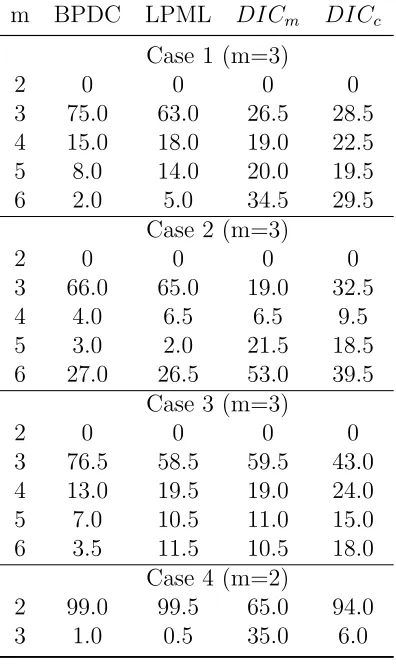
Table 3.1 Percentage of model selection decisions (Case 1-4) . . . 56

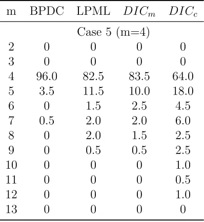
Table 3.2 Percentage of model selection decisions (Case 5) . . . 57

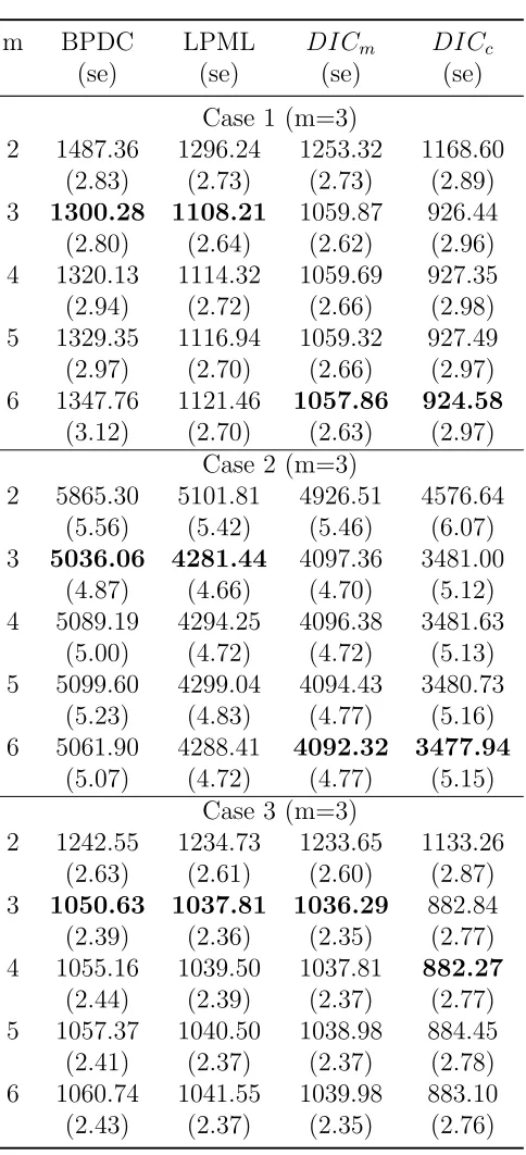
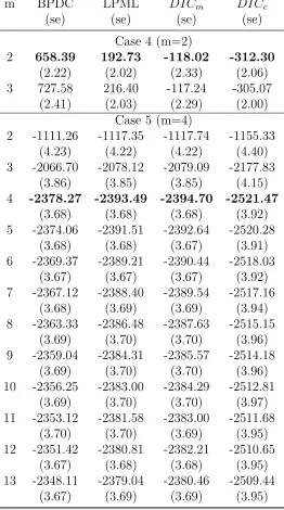
Table 3.3 Average of model selection criteria and standard errors (Case 1-3) . 58 Table 3.4 Average of model selection criteria and standard errors (Case 4-5) . 59 Table 3.5 Fit of Gaussian process with nonlinear mean and covariance functions 61 Table 3.6 BPDC of models on Sitka data . . . 67

Table 4.1 Percentage of model selection decisions for missing data models (Case 1-3) . . . 89

Table 4.2 Average of model selection criteria and standard errors for missing data models (Case 1-2) . . . 90

Table 4.3 Average of model selection criteria and standard errors for missing data models (Case 3) . . . 91

Table 4.4 Percentage of model selection decisions for censored data models (Case 1-3) . . . 92

Table 4.5 Average of model selection criteria and standard errors for censored data models (Case 1-2) . . . 93

Table 4.6 Average of model selection criteria and standard errors for censored data models (Case 3) . . . 94

Table 4.7 Sample size across weeks of the schizophrenia study. . . 96

Table 4.8 BPDC of models for schizophrenia study . . . 98

(11)

LIST OF FIGURES

Figure 1.1 Left: the growth curves of Sitka spruce trees. Right: the HIV viral load across weeks, where the light blue shaded area highlights those unreliable measurements. . . 2 Figure 1.2 First row: covariance functions; (1)KSE(t, s) = exp{−(t−s)2/2},

(2)KS(t, s) = exp{−sin2(π|t−s|)/2}, and (3)KBB(t, s) = min(t, s)+ ts. Second row: three random functions drawn from corresponding centered Gaussian processes. . . 11 Figure 2.1 Bernstein basis polynomials of degree 2 and degree 7 . . . 17 Figure 2.2 Pm

i=0 √

λiV1(ei) is plotted againstmfor the square exponential kernel. 35

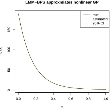
Figure 3.1 Estimated mean function is plotted in dashed red along with its pointwise 95% credible interval in dashed green lines. The true mean curve is displayed in solid black line. . . 62 Figure 3.2 Growth curves of Sitka spruce trees over days. Black: the ozone

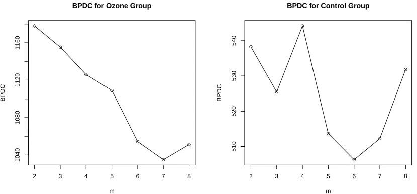
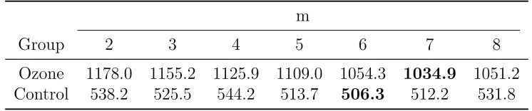
group. Red: the control group. . . 63 Figure 3.3 BPDC of models for ozone and control group . . . 66 Figure 3.4 Left: estimated mean function over days, and original observations

displayed to show the fit of the model. Right: estimated difference function and its 95% credible interval where the difference func-tion is the mean funcfunc-tion of ozone group minus the mean funcfunc-tion of control group and the grey line is the reference line at y=0. The fixed treatment effect obtained by Crainiceanu et al. (2005) is shown in blue dashed line at y=0.31. . . 68 Figure 3.5 Estimated covariance function over days. Left: ozone group. Right:

control group . . . 69 Figure 3.6 Left: estimated mean function of growth rate over days. Right:

estimated difference function of growth rate and its 95% credible interval and the grey line is the reference line at y=0. . . 70 Figure 3.7 Growth curves of females and males from age 1 to 18. Black: the

female group. Red: the male group. . . 72 Figure 3.8 BPDC of models for female and male group. . . 72 Figure 3.9 Left: estimated mean growth function of children over ages. Right:

estimated difference function between females and males and its 95% credible interval. The grey line is the references line at y=0. . 73 Figure 3.10 Left: estimated mean function of growth rate over ages. Right:

(12)

Figure 4.1 Severity scores across weeks for the first 8 patients in each group. Solid segments are used to link two measurements in the neigh-borhood, and dashed segments are used to link two measurements with missing values in the middle. . . 96 Figure 4.2 Left: estimated mean function over weeks, and original group means

by week displayed to show the fit of the model. Right: estimated difference function between placebo group and drug group along with its 95% credible interval and the reference line in grey at y=0. 99 Figure 4.3 Estimated covariance functions over weeks. Left: placebo group.

Right: drug group . . . 99 Figure 4.4 Left: estimated first derivative of mean function over weeks. Right:

estimated difference of the first derivative function between placebo group and drug group along with its 95% credible interval. . . 100 Figure 4.5 Log10 of HIV viral load (copies/ml) across weeks. The SPI group

is plotted in solid black line, while DPI group is plotted in dashed red line. Horizontal reference line in blue is plotted at log₁₀(200) copies/ml where measurements below the line is inaccurate. The light blue shaded area highlights those measurements which are not reliable. . . 101 Figure 4.6 Estimated mean functions over weeks. Left: NNTRI-naive group;

Right: NNTRI-experienced group. . . 105 Figure 4.7 Estimated differences between mean functions of SPI and DPI

(13)

Chapter 1 Mixed Effects Models for

Longitudinal Study

1.1 Introduction

(14)

One interesting feature about this data set is that the growth curve must necessarily be nondecreasing and such shape constraints must be accommodated in statistical models. Some other longitudinal data have spontaneous shape restrictions as well, such as the hearing loss study analyzed in Davidov and Rosen (2011). The ACTG 398 data analyzed by Sun and Wu (2005) is another typical longitudinal data set which involves about 22% left-censored observations. In the right panel of Figure 1.1, it is clear that the curves tangle in a mess, where no obvious pattern can be identified simply by looking at the plot. In practice, longitudinal data are usually subject to data irregularities such as miss-ing, censored and truncated values. This requires suitable methodologies to handle the missing/censoring/truncating mechanism, and appropriate analysis is needed for making probabilistically valid statistical inference. The two examples described above are typical real data scenarios, and in general such longitudinally observed data can be modelled within a general statistical framework.

● ● ● ● ● ● ● ● ● ● ● ● ●

200 300 400 500 600 700

2 3 4 5 6 7 8 Sitka Data t(days) y(log−siz e) ● ● ● ● ● ● ● ● ● ● ● ● ● ● ● ● ● ● ● ● ● ● ● ● ● ● ● ● ● ● ● ● ● ● ● ● ● ● ● ● ● ● ● ● ● ● ● ● ● ● ● ● ● ● ● ● ● ● ● ● ● ● ● ● ● ● ● ● ● ● ● ● ● ● ● ● ● ● ● ● ● ● ● ● ● ● ● ● ● ● ● ● ● ● ● ● ● ● ● ● ● ● ● ● ● ● ● ● ● ● ● ● ● ● ● ● ● ● ● ● ● ● ● ● ● ● ● ● ● ● ● ● ● ● ● ● ● ● ● ● ● ● ● ● ● ● ● ● ● ● ● ● ● ● ● ● ● ● ● ● ● ● ● ● ● ● ● ● ● ● ● ● ● ● ● ● ● ● ● ● ● ● ● ● ● ● ● ● ● ● ● ● ● ● ● ● ● ● ● ● ● ● ● ● ● ● ● ● ● ● ● ● ● ● ● ● ● ● ● ● ● ● ● ● ● ● ● ● ● ● ● ● ● _● ● ● ● ● ● ● ● ● ● ● ● ● ● ● ● ● ● ● ● ● ● ● ● ● ● ● ● ● ● ● ● ● ● ● ● ● ● ● ● ● ● ● ● ● ● ● ● ● ● ● ● ● ● ● ● ● ● ● ● ● ● ● ● ● ● ● ● ● ● ● ● ● ● ● ● ● ● ● ● ● ● ● ● ● ● ● ● ● ● ● ● ● ● ● ● ● ● ● ● ● ● ● ● ● ● ● ● ● ● ● ● ● ● ● ● ● _● ● ● ● ● ● ● ● ● ● ● ● ● ● ● ● ● ● ● ● ● ● ● ● ● ● ● ● ● ● ● ● ● ● ● ● ● ● ● ● ● ● ● ● ● ● ● ● ● ● ● ● ● ● ● ● ● ● ● ● ● ● ● ● ● ● ● ● ● ● ● ● ● ● ● ● ● _● ● ● ● ● ● ● ● ● ● ● ● ● ● ● ● ● ● ● ● ● ● ● ● ● ● ● ● ● ● ● ● ● ● ● ● ● ● ● ● ● ● ● ● ● ● ● ● ● ● ● ● ● ● ● ● ● ● ● ● ● ● ● ● ● ● ● ● ● ● ● ● ● ● ● ● ● ● ● ● ● ● ● ● ● ● ● ● ● ● ● ● ● ● ● ● ● ● ● ● ● ● ● ● ● ● ● ● ● ● ● ● ● ● ● ● ● ● ● ● ● ● ● ● ● ● ● ● ● ● ● ● ● ● ● ● ● ● ● ● ● ● ● _● _● ● ● ● ● ● ● ● ● ● ● ● ● ● ● ● ● ● ● ● ● ● ● ● ● ● ● ● ● ● ● ● ● ● ● ● ● ● ● ● ● ● ● ● ● ● ● ● ● ● ● ● ● ● ● ● ● ● ● ● ● ● ● ● ● ● ● ● ● ● ● ● ● ● ● ● ● ● ● ● ● ● ● ● ● ● ● ● ● ● ● ● ● ● ● ● ● ● ● ● ● ● ● ● ● ● ● ● ● ● ● ● ● ● ● ● ● ● ● ● ● ● ● ● ● ● ● ● ● ● ● ● ● ● ● ● ● ● ● ● ● ● ● ● ● ● ● ● ● ● ● ● ● ● ● ● ● ● ● ● ● ● ● ● ● ● ● ● ● ● ● ● ● ● ● ● ● ● ● ● ● ● ● ● ● ● ● ● ● ● ● ● ● ● ● ● ● ● ● ● ● ● ● ● ● ● ● ● ● ● ● ● ● ● ● ● ● ● ● ● ● ● ● ● ● ● ● ● ● ● ● ● ● ● ● ● ● ● ● ● ● ● ● ● ● ● ● ● ● ● ● ● ● ● ● ● ● ● ● ● ● ● ● ● ● ● ● ● ● ● ● ● _● ● ● ● ● ● ● ● ● ● ● ● ● ● ● ● ● ● ● ● ● ● ● ● ● ● _● ● ● ● ● ● ● ● ● ● ● ● ● ● ● ● ● ● ● ● ● ● ● ● ● ● ● ● ● ● ● ● ● ● ● ● ● ● ● ● ● ● ● ● ● ● ● ● ● ● ● ● ● ● ● ● ● ● ● ● ● ● ● ● ● ● ● ● ● ● ● ● ● ● ● ● ● ● ● ● ● ● ● ● ● ● ● ● ● ● ● ● ● ● ● ● ● ● ● ● ● ● ● ● ● ● ● ● ● ● ● ● ● ● ● ● ● ● ● ● ● ● ● ● ● ● ● ● ● ● ● ● ● ● ● ● ● ● ● ● ● ● ● ● ● ozone control

0 5 10 15 20

2

4

6

8

ACTG 398 Study

week

log10 HIV vir

al load

SPI DPI

(15)

For each randomly sampled subjecti, letYi(t) denote the measured response obtained

at time t ∈ [0, T] for i = 1, . . . , I. Let Zi = (Zi1, . . . , Zip)T denote a vector of baseline

covariates measured at time point t = 0 for the subject i. More generally, we may also have time-varying covariates measured at time t denoted as Zi(t) and the goal of the

study would be exploring the relationship between Y(t) and Z(t). However, for the sake of simplicity, we first assume only baseline covariates are included in the study. For example, for the Sitka spruce trees study, we have p = 1 and the binary covariate Zi

indicating an ozone-enriched environment or natural environment. One may start with postulating the following statistical model:

Yi(t) = ZiTβ+Xi(t) +i(t), i= 1, . . . , I, (1.1)

where {Xi(t) : t ∈ [0, T]} are independently and identically distributed (iid) as the

stochastic process {X(t) : t ∈ [0, T]} and {i(t) : t ∈ [0, T]} are iid as a white noise

process. More precisely, we assumeE[i(t)] = 0 for anyiand anytandCov[i(t), j(t)] = σ2_δ

ijδts where δab = 1 if a =b and δab = 0 otherwise for a, b∈R. One of the main goals

of the study is to model the latent stochastic process {X(t) :t∈[0, T]}.

One of the challenging aspects of estimating model (1.1) is that the response process

Yi(t) is not observed for all time points t∈[0, T] and the collection of time points could also vary with the subject i. Such feature of the data prohibits the use of standard off-the-shelf multivariate analysis for growth curve models. In general, we may observe Yi(t)

measured only at a selected set of time points ti1 < ti2 < . . . < tiJi where Ji ≥ 2 for

i = 1, . . . , I. Let Yij = Yi(tij) for i = 1, . . . , I and j = 1, . . . , Ji, and the observed data

(16)

postulate the following model:

Yij =ZiTβ+Xij +ij, i= 1, . . . , I, j = 1, . . . , Ji, (1.2)

where ij iid∼ (0, σ2) and the goal would be estimating parameter of the latent stochastic process{X(t) :t∈[0, T]}and (β, σ2_{) based on the data}

D. Parametric approaches assume

that Xi = (Xi1, . . . , XiJi)

T ₌ _U

ibi, where Ui = (Ui1, . . . , Uiq) denotes a Ji ×q matrix

designed to capture the trend andbi denotes random effects to capture the heterogeneity

across subjects. This reduces the model (1.2) to the following linear mixed effects model (LMM),

Yi = ZiTβ+Uibi+i, i= 1, . . . , I. (1.3)

Following common practice, we assume bi

iid

∼ N(0,Σb) and i

ind

∼ N(0, σ2_I_{). Many} stan-dard software packages are available (e.g. PROC MIXED in SAS, lme in R, etc.) which allows the estimation of the parameters θ = (β,Σb, σ2) using maximum likelihood (ML;

Robinson 1991), restricted maximum likelihood (REML; Patterson and Thompson 1971; Harville 1977), or EM algorithm (Lindstrom and Bates 1988).

Clearly, the models described in (1.2) and (1.3) are based on the linearity assump-tion that relates Yi’s to Zi’s and Ui’s, which usually provides a very good first order

approximation. Model (1.3) has been generalized to approximate more complex relation-ship between the responses (Yi’s), baseline covariates (Zi’s) and trend variables (Ui’s).

More generally, we may consider the following so called nonlinear mixed effects model (NLMM),

(17)

where g(·) is a known function, bi’s are subject specific random effects to capture

varia-tions across subjects, and β is a vector of fixed effects capturing the baseline effects. As in model (1.3) we have similar assumptions regarding the bi’s andi’s to be independent

to each other for i= 1, . . . , I. See Davidian and Giltinan (1995), Davidian and Giltinan (2003), and Serroyen et al. (2009) for comprehensive reviews on NLMM with various ap-plications in practice. When we can identify the form ofg(·) from the mechanistic theory, the parametric NLMM is employed. Some typical applications include the pharmacoki-netics and pharmacodynamic modeling (Davidian and Giltinan 1995, Chpater 5), HIV dynamics modelling (Han and Chaloner 2004), and prostate specific antigen modeling (Morrell et al. 1995). Moreover, classical NLMM can be implemented directly in some popular statistical software, such as PROC NLMIXED in SAS and nlme in R. However, the assumption that the functional form of the nonlinear relationship is known may often turn out to be restrictive. Misspecified nonlinear relationship is likely to cause improper use of NLMM. Ke and Wang (2001) proposed a semiparameteric NLMM and applied their model to AIDS data, where only the mean function is modelled nonparametrically. A nonparametric NLMM was proposed by Lindstrom (1995), which replaced the nonlin-ear function with a free-node spline shape function. But the resulting covariance structure fitted in this way is not easy to interpret.

In general, although model (1.4) provides a greater flexibility in capturing the possible relationships between the responses (Yi’s), baseline covariates (Zi’s) and trend variables

(Ui’s), the model is still based on an assumed nonlinear functional form which may only

(18)

with, we focus on modeling the latent stochastic process X(t) in model (1.1). A widely used model to approximate a continuous stochastic process is given by the Gaussian process which is characterized by specifying a mean function and a covariance function. Next we provide a brief review of Gaussian processes in Section 1.2 and a class of nonlinear mixed effects models based on Gaussian processes (NLMM-GP) is introduced in Section 1.3. Finally, in Section 1.4, the organization of the whole dissertation is outlined.

1.2 Gaussian Processes

Gaussian distribution is one of the well-known distributions in statistics and has been widely used in many practical scenarios involving measured responses subject to random errors. A finite dimensional vector X = (XI, . . . , Xm)T is said to have a multivariate Gaussian distribution if a linear function a1X1 +. . .+amXm has a univariate Gaussian

distribution for any a = (a1, . . . , am)T ∈ Rm (Casella and Berger 2001, Chapter 4).

Extending this definition to a stochastic process {X(t);t ∈ [0, T]}, we would say that it is a Gaussian process if every finite dimensional vector (X(t1), . . . , X(tm))T has a

multivariate Gaussian distribution for any finite set of distinct t1, . . . , tm ∈[0, T]. It can

be shown that a Gaussian process is characterized by its mean function µ(t) =E[X(t)] and covariance function K(t, s) = Cov(X(t), X(s)).

Definition 1.2.1. A stochastic process {X(t);t ∈ [0, T]} is said to be a Gaussian

pro-cess with mean function µ(t) and covariance function K(t, s) if for any finite collection

t1, . . . , tm ∈[0, T], the vector (X(t1), . . . , X(tm))T has a multivariate Gaussian

(19)

We denote this stochastic process by the notation

X(·)∼GP(µ(·), K(·,·)).

Rasmussen and Williams (2006) demonstrated that Gaussian processes can be used to approximate many well-known statistical models, including Bayesian linear models, spline models, large neural networks (under suitable conditions), and are closely related to other popular models, such as support vector machines. The linear mixed effects model (1.3) is also a special case of Gaussian processes. Assuming random variables are drawn from a Gaussian process always makes the model easy to handle and interpret. “Under the Gaussian process viewpoint, the models may be easier to handle and interpret than their conventional counterparts, such as e.g. neural networks.” (Rasmussen and Williams 2006). As Gaussian distribution can approximate many real world random phenomenon, the widespread use of Gaussian processes is always considered reasonable for longitudinal analysis, spatial analysis, and computer experiments analysis, among others. So we begin with the assumption that Xi(·)

iid

∼ GP(µ(·), K(·,·)) within any modeling framework as described in (1.1) One of the main stumbling block of this generalization is that we need to estimate the mean functionµ(·) and the covariance functionK(·,·) based on the observed data_D ={(Yij, tij, Zi) :i = 1, . . . , I;j = 1, . . . , Ji}, whereZi = (Zi1, . . . , Zip)T. The mean function can be assumed to belong to a suitable class of smooth function (e.g. continuous functions on [0, T], etc). But the covariance function needs to be a non-negative definite (nnd) function, also known as a valid kernel.

(20)

(nnd) function if and only if K(t, s) = K(s, t) for any s, t∈[0, T] and

m X

i,j=1

aiajK(ti, tj)≥0 (1.5)

for any set of points {t1, . . . , tm} in [0, T] and for any set of real numbers {a1, . . . , am}. A nnd function can be characterized by its spectral decomposition by extending the idea of spectral decomposition of a nnd matrix. The characterization is given by the celebrated Mercer’s Theorem (restated by Minh et al. 2006).

Theorem 1.2.1. Mercer’s Theorem.LetK be a continuous nonnegative definite

func-tion on [0, T]×[0, T] satisfying

Z T

0

Z T

0

K2(s, t)dw(s)dw(t)<∞, (1.6)

wherew(·)is an absolutely continuous weight function defined on[0, T]. Then, there exists a sequence of orthogonal functions {ek(t);k = 1,2, . . .;t∈[0, T]} satisfying

Z T

0

ek(t)el(t)dw(t) =δkl

and a sequence of nonnegative real numbers {λk :λk≥0;k = 1,2, . . .} such that

K(s, t) =

∞ X

k=1

λkek(s)ek(t), (1.7)

where the infinite series converges absolutely for each pair (s, t)∈ [0, T]2 and uniformly on each compact subset of [0, T]2_.

(21)

are known as the eigenvalues ofK.

Eigenvalues and eigenfunctions defined in Theorem 1.2.1 can be obtained by solv-ing the integral equations R₀T K(t, s)e(s)dw(s) = λe(t) and R₀T e2₍_t₎_dw₍_t_{) = 1. For} ex-ample, the Wiener process defined on [0,1] has the kernel K(t, s) = min(t, s), whose eigenfunctions and eigenvalues are {ek(t) =

√

2 sin((k − 1

2)πt);k = 1, . . .} and {λk = [(k− 1

2)

2_π2_]−1_;_k _{= 1}_{, . . .}_{}, when the weight function is the Lebesgue measure. Also in} virtue of Mercer’s Theorem, Lo`eve (1945) and Karhunen (1947) introduced Karhunen-Lo`eve (K-L) expansion of a stochastic process which allows us to represent a stochastic process using a countable number of real numbers and sequence of orthogonal functions.

Theorem 1.2.2. Karhunen-Lo`eve (K-L) expansion of a stochastic process. Let

X(t) be a second-order stochastic process defined over a probability space (Ω,F, P) and indexed over a closed and bounded interval[0, T]with continuous mean functionµ(·)and covariance function K(·,·)satisfying the assumptions in Theorem 1.2.1. Then, X(t) has a (quadratic mean) representation in terms of L2 norm.

X(t) = µ(t) +

∞ X

k=1

p

λkek(t)Zk, (1.8)

where the random variables Zk’s satisfying

√

λkZk = RT

0 X(t)ek(t)dw(t) have zero-mean, and are uncorrelated with variance 1. In other words, E[Zk] = 0 and Cov(Zk, Zl) = δkl

for any k and l.

Remark: If we further assume that X(·) ∼ GP(µ(·), K(·,·)), then random variables {Zk;k= 1,2, . . .} are iid as standard normal distribution, i.e.Zk iid∼N(0,1).

There are several popular kernel functions including squared exponential kernel

(22)

kernelKS(t, s) = σ2exp{−ksin2(π|t−s|)}, and the kernel to a centered Brownian bridge KBB(t, s) = min(t, s) +ts, among others. Figure 1.2 displays three valid kernel functions

and three random functions drawn from the corresponding GP(0, K(·,·)). It shows that with various kernel functions we can mimic a variety of shapes for random functions.

Another interesting fact about Guassian process is that if the second order deriva-tive ∂2_∂t∂sK(t,s) exists for all pairs of points (s, t) ∈ [0, T]×[0, T], then the derivative of a Gaussian process is still a Gaussian process. This is true because differentiation is a linear operation (Solak et al. 2003). Suppose X(t) ∼ GP(µ(·), K(·,·)) where µ(·) and

K(·,·) are differentiable, then the derivative of X(t) also forms a Guassian process,

X0(t) ∼ GP(µ∗(·), K∗(·,·)), where µ∗(t) = µ0(t) and K∗(t, s) = ∂2_∂t∂sK(t,s). This property enables us to analyze the derivative of a Gaussian process, e.g., the growth rate (deriva-tive of the growth curve). One the other side, we can also take advantage of the fact when we have the derivative observations, e.g., the perturbation data (Solak et al. 2003).

1.3 Parameter Estimation using Gaussian Process

Models

(23)

−2 −1 0 1 2 −2 −1 0 1 2 0.2 0.4 0.6 0.8 1.0

A Squared Exponential Kernel

−2 −1 0 1 2

−2 −1 0 1 2 t y −2 −1 0 1 2 −2 −1 0 1 2 0.7 0.8 0.9 1.0

A Seasonal Kernel

−2 −1 0 1 2

−1 0 1 2 t y 0.0 0.2 0.40.6 0.81.0 0.0 0.2 0.4 0.6 0.8 1.0 0.0 0.5 1.0 1.5 2.0

Brownian Bridge Kernel

0.0 0.2 0.4 0.6 0.8 1.0

−2 −1 0 1 t y

Figure 1.2: First row: covariance functions; (1) KSE(t, s) = exp{−(t − s)2/2}, (2) KS(t, s) = exp{−sin2(π|t − s|)/2}, and (3) KBB(t, s) = min(t, s) + ts. Second row:

three random functions drawn from corresponding centered Gaussian processes.

the baseline (or time-varying) covariates,

Yi(t) = Xi(t) +i(t), t ∈[0, T], i= 1, . . . , I, (1.9) Xi(t)

iid

∼ GP(µ(·), K(·,·)), i(t) iid∼ W N(σ2),

whereW N(σ2_{) denotes a white noise process with mean zero and variance}_σ2_{. For} exam-ple, we may assume i(t) to be a Gaussian process with mean function identically zero

and covariance function K(t, s) = σ2δts.

(24)

(Yi(ti1), . . . , Yi(tiJi))

T _for _i_{= 1}_{, . . . , I} _and _J

i ≥2. Then model (1.9) becomes

Yij = Xi(tij) +ij, i= 1, . . . , I, j = 1, . . . , Ji, (1.10)

(Xi(ti1), . . . , Xi(tiJi))

T ind

∼ N (µ(ti1), . . . , µ(tiJi))

T_,₍_K₍_t

ij, tij0))₁_≤j,j0_≤J

i

,

ij

iid

∼ N(0, σ2).

With Model (1.10), we have modelled the fixed effects with µ(·), which is also the population mean function, and the random effects with K(·,·), which also describes the variation within and across the subjects. We only pose minimal restrictions on the mean function µ(·) and covariance function K(·,·), so that we can approximate any underly-ing Gaussian process that generates Xi(t). In addition, linear mixed effects models are

special cases of model (1.10). Though the NLMM Model (1.4) may not belong to the class of nonlinear mixed effects models based on Gaussian processes (NLMM-GP), we can still approximate them as well as other stochastic processes with Model (1.10) up to the first two moment functions. Compared to Model (1.4) where we need to develop methodology for every specific model, NLMM-GP is easier to be handled by a general method for estimation and statistical inference. In general, NLMM-GP is flexible enough to approximate most of the Gaussian processes and accommodate other stochastic pro-cesses up to the first two moments. What’s more, its estimation and statistical inference is easy since it eventually reduces to finite-dimensional Gaussian distributions.

A commonly used method involves specifying the mean function µ(·) and the covari-ance functionK(·,·) parametrically and then estimating the parameters with a likelihood based approach (Casella and Berger 2001, Chapter 7) or an estimating equation based approach (Godambe 1991) or a Bayesian approach (Inusa et al. 2012, Chapter 2). More specifically, suppose we assume µ(t) = Pp

k=1φk(t)βk and K(t, s) = Pq

(25)

where {φk(t);k = 1,2, . . .;t ∈ [0, T]} forms an orthogonal basis with respect to the

weight functionw(t),t ∈[0, T], say,RT

0 φk(t)φl(t)dw(t) =δkl. Then Model (1.10) can be represented as

Yij = p X

h=1

φh(tij)βh+ q X

k=1

p

λkφk(tij)Zik+σij, (1.11)

where Zik, ij

iid

∼N(0,1), β = (β1, . . . , βp)T ∈Rp, and λ= (λ1, . . . , λq)T ∈[0,∞).

Note that Model (1.11) can be written in vector form,

Yi = Fiβ+ei, (1.12)

ei

ind

∼ N(0, FiD(λ)FiT +σ2I),

whereFi = (φk(tij)) is a Ji×pmatrix with (j,k)th entry φk(tij). We can use a likelihood

based method (e.g. maximum likelihood method or Bayesian method) to estimate the model parameters θ= (β, λ, σ2₎_∈

Rp×[0,∞)q×[0,∞). Although the above framework

provides a very flexible class of models to approximate a Gaussian process, there are at least couple of limitations. First, we need to suitably choose the class of orthogonal basis {φk(t);k = 1,2, . . .;t∈ [0, T]}. Second, we need to select the truncation orders pand q.

One of the major goals of the dissertation is to overcome the above two limitations by simultaneously estimating theµ(·) and K(·,·) under some mild regularity conditions.

1.4 Organization of the Dissertation

(26)

discussion on- definition and properties of the Gaussian processes, a class of nonlinear mixed effects models based on Gaussian process is introduced and compared to other NLMM’s. In Chapter 2, a class of linear mixed effect models using Bernstein polynomial sieve (LMM-BPS) is proposed to approximate the class of NLMM-GP. The convergence properties of the LMM-BPS are explored in terms ofLp norms for 1≤p < ∞. In Chapter

(27)

Chapter 2 Gaussian Processes Approximation

with Bernstein Polynomials

2.1 Introduction

(28)

zero variance components in order to select the number of eigenfunctions. Crainiceanu and Goldsmith (2010) applied the functional principal component analysis on the sleep EEG data for 500 subjects. However, to implement FPCA, we need to use empirical estimates of eigenfunctions in the first place which may cause problem when sample size is not large and when observations are very sparse or missing or censoring. Also in Crainiceanu and Goldsmith (2010)’s example, they used the sample mean at every time point to estimate the mean function, which is too rough and hard to interpret. We cannot make conclusion about the population trend based on their model. One of the most common limitations of the FPCA is that these methods are primarily based on two stages of estimations: first the eigenfunctions are estimated and then these estimated functions are plugged-in to estimate the mean function or to predict the future observations. To overcome some of these limitations, first we establish a result based on Bernstein polynomial sieve to show the Lp−norm approximation of a Gaussian process. Then we illustrate that

Bern-stein polynomial sieve based approximation can be written within a linear mixed effects model framework. To start with, we provide a brief overview on the theory of Bernstein polynomial based approximations.

2.2 Bernstein Polynomials

(29)

2.2.1 Definition and Convergency Properties

The Bernstein basis polynomials of degreem−1 is defined as

bk,m(t) =

m−1

k−1

tk−1(1−t)m−k, k = 1, . . . , m, t∈[0,1]. (2.1)

Figure 2.1 gives the plots of Bernstein basis polynomial sieve of degree m−1 form = 3 and m = 8 respectively. The Bernstein polynomials of degree m−1 is defined as any

0.0 0.2 0.4 0.6 0.8 1.0

0.0

0.2

0.4

0.6

0.8

1.0

Bernstein Basis Polynomials of Degree 2

t

y

k=1 k=2 k=3

0.0 0.2 0.4 0.6 0.8 1.0

0.0

0.2

0.4

0.6

0.8

1.0

Bernstein Basis Polynomials of Degree 7

t

y

k=1 k=2 k=3 k=4 k=5 k=6 k=7 k=8

Figure 2.1: Bernstein basis polynomials of degree 2 and degree 7

linear combination of Bernstein basis polynomials,

Bm(t) = m X

k=1

ak,mbk,m(t), t∈[0,1], (2.2)

where ak,m can be any real number. Any BP is continuous and infinitely many

(30)

BP of a lower degree. In other words,

B_m0 (t) = (m−1)

m−1

X

k=1

(ak+1,m−ak,m)bk,m−1(t). (2.3)

More generally, the l-th order derivative is still a BP and given by

B_m(l)(t) =l!

m−1

l

m−l

X

k=1

∇(l)ak,mbk,m−l(t), (2.4)

where ∇(l)_a

k,m = ∇(l−1)ak+1,m− ∇(l−1)ak,m for l = 1,2, . . .. From above, it follows that

linear restrictions on the coefficientsak,m’s induce restrictions on the derivatives ofBm(t)

for t ∈ [0,1]. For example, if a1,m ≤ a2,m ≤ . . . ≤ am,m, then B0m(t) ≥ 0 for t ∈ [0,1].

Thus shape constraints like nonnegativity, monotonicity, and convexities can be easily imposed by using finite dimensional linear inequality constraints on the coefficients.

One of the most celebrated results in real analysis is that the sequence of polynomials are dense for the space of continuous functions on a compact interval, which is known as the Weierstrass Approximation Theorem. Bernstein (1912) provided a constructive proof of this celebrated result which we state below.

Theorem 2.2.1. Bernstein Weierstrass Approximation Theorem,(Lorentz, 1953,

Chapter 1). Let f : [0,1]→_R be a bounded function and consider the Bernstein polyno-mial given by

Bm(f, t) = m X

k=1

f

k−1

m−1

(31)

Then,

lim

m→∞Bm(f, t) =f(t) (2.6)

holds at each point of continuity of f(t); and the convergence holds uniformly on any [a, b]⊆[0,1] if f(t) is continuous on [a, b].

Bm(f, t) defined in Theorem 2.2.1 is also known as the Bernstein polynomial of

func-tion f. With Equation (2.5), we see that the Bernstein polynomial of a function reduces the estimation of the entire function to a finite dimensional problem. It also enables the shape-preserving property of Bernstein polynomials, which we introduce later in Section 2.2.2. We also state some well-known results that provide the order of approximation.

Theorem 2.2.2. The Degree of Approximation by Bernstein Polynomials,

(Lorentz, 1953, Chapter 1). Let f : [0,1] → _R has a continuous derivative f0(t) in [0,1]. If f0(t) satisfies the Lipschitz condition of order 1 on [0,1] such that

|f0(t1)−f0(t2)| ≤A|t1−t2|, t1, t2 ∈[0,1], (2.7)

where A is a constant. Then,

|Bm(f, t)−f(t)| ≤C(m−1)−1, (2.8)

where C is a constant.

(32)

If a function defined on [a, b] is continuous, we can define

Bm(f, x) = m X

k=1

f

a+ (b−a)(k−1)

m−1

bk,m

x−a b−a

. (2.9)

Equation (2.9) is obtained through the linear transformation t = (x−a)/(b −a) such that t ∈ [0,1]. Babu et al. (2002) suggested to use transformation t = x/(1 + x) and

t = 1/2 + (1/π) tan−1₍_x_{) to map [0}_,_{∞) and (−∞}_,_{∞) to [0}_,_{1] respectively. In practice} we may use t= (x−a)/(b−a) where a and b are “estimated” from the observed values ofx’s. After the transformation, the support set is always condensed or enlarged to [0,1], which is of length 1.

Theorem 2.2.1 provides the convergence properties of Bernstein polynomials in L∞

norm. Hoeffding (1971) discussed the L1 norm approximation error for Bernstein poly-nomials. Jones (1976) proved several theorems for the approximation error of Bernstein polynomials inL2 norm. Khan (1985) proved some results in terms ofLp norm for p≥1.

Some important results are listed below.

Theorem 2.2.3. The L1 norm of the Bernstein polynomials approximation,

Hoeffding (1971). Let f be of bounded variation in [0,1]. Then

Z 1

0

|Bm(f, t)−f(t)|dt≤CmJ(f) +m−1V ar[0,1](f)1, (2.10)

whereJ(f) =R₀1t1/2₍₁₋_t₎1/2_d_|_f₍_t_)|_and_C

m = 21/2(m−1/2)m−1/2m−m < p

2/[(m−1)e].

Conditions 2.2.1. Condition T, Jones (1976). We say a function f(t) satisfies

con-dition T at a point p ∈ [0,1] if (a) for any > 0 there exist τ > 0 and 0 < q < 1

1_{V ar}

[0,1](f) is the total variation of f on [0,1], defined as supP

Pm−1

i=1 |f(ti+1)−f(ti)|, where P =

(33)

such that for any t1, t2 ∈ (0,1) satisfying 0 < q(p −t2) < p−t1 < p− t2 ≤ τ or 0< q(t2−p)< t1−p < t2−p≤τ, |f(t1)/f(t2)−1| ≤ holds, and (b) there exist γ >0,

M >0, a≥0 such that for 0<|p−t|< γ, t∈(0,1), f(t)≥M|u−p|a _holds.

Theorem 2.2.4. The L2 norm of the Bernstein polynomials approximation,

Jones (1976). Let f be an absolutely continuous function on (0,1) with derivative f0. Suppose f and f0 satisfy the conditions

(i) f is bounded on [0,1]and there exist δ >0and t0 ∈(0,1)such that |f(t)−f(0)| ≤

Ktδ_, _|_f₍_t₎₋_f_{(1)| ≤}_K₍₁₋_t₎δ _for ₀_≤_t_≤_t

0, and some K >0,

(ii) f0 is continuous on (0,1), satisfies Condition 2.2.1, part (a) at 0 and 1, (iii) J2(f) =

R1 0[f

0₍_t_)]2_t₍₁₋_t₎_{dt <}_∞. Then

Z 1

0

[Bm(f, t)−f(t)]2dt ≤m−1J2(f) +o(m−1).

Theorem 2.2.5. The Lp norm of the Bernstein polynomials approximation,

Khan (1985). Let f(t)be a continuous function on [0,1] with continuous derivative f0(t). Define Dp_m(f, t) = Pm

k=1|f(

k−1

m−1)−f(t)|

p_b

m,k(t), and Vp(f) = R1

0 t

p/2₍₁₋_t₎p/2_|_f0₍_t_)|p_dt_.

Then

mp/2D_mp(f, t)→Cptp/2(1−t)p/2|f0(t)|p as m→ ∞,

and

lim

m→∞m

p/2

Z 1

0

Dp_m(f, t)dt=CpVp(t),

for 1≤p <∞, where Cp = 2p/2Γ((p+ 1)/2)/

√

(34)

With Theorems 2.2.1, 2.2.3, 2.2.4, and 2.2.5 we are able to explore convergence prop-erties of Bernstein polynomials approximation for Gaussian processes.

2.2.2 Shape-preserving Properties

Another attractive property of Bernstein polynomials is its optimal shape restriction property among all polynomials (Carnicer and Pena 1993). Chapter 1, Gal (2008) pro-vided complete proofs to many shape-preserving properties and some other interest-ing properties. Wang (2012) also elaborated some of the interestinterest-ing results on convex functions, quasi-convex functions, monotone functions, and u-monotone function where

u(t) =tλ, λ∈(0,1). They showed that to estimate a shape-restricted function with cer-tain pattern using Bernstein polynomials we only need to put some restrictions on the coefficients of the Bernstein polynomials. For example, if f(t) is an unknown continu-ous increasing function on [0,1], then Bm(f, t) is also a continuous increasing function.

The coefficients of Bm(f, t) are {f(0), f(_m−1₁), . . . , f(1)}, which is also an increasing

se-quence. Therefore, we just need to restrict the Bernstein polynomial coefficients to satisfy

a1,m< a2,m < . . . < am,mif we try to find a Bernstein polynomial that approximatesf(t).

Iff(t) is an unknown nonnegative function, then Bm(f, t) is also a nonnegative function

with nonnegative coefficients. Hence, we require ak,m ≥ 0 for k = 1, . . . , m. If f(t) is a convex function such that 2f(t1+t2

2 ) ≤ f(t1) +f(t2), then Bm(f, t) is also a convex function. In this case, we enforce ak,m−2ak+1,m+ak+2,m≥0 for k= 1, . . . , m−2. There

(35)

selection, and other areas.

2.3 A Class of Linear Mixed Effects Models with

Bernstein Polynomial Sieve

(36)

polynomials (LMM-BPS) to replace Model (1.10),

Yij = m X

k=1

bkm(tij)βik+ij, i= 1, . . . , I;j = 1, . . . , Ji, (2.11) βi

iid

∼ N(β0, D),

i inid∼ N(0, σ2_iI),

where βi = (βi1, . . . , βim)T, β0 = (β01, . . . , β0m)T and i = (i1, . . . , im)T. With Model

(2.11), we have approximated X(t) with Gaussian process

GP m X

k=1

bkm(t)β0k, m X

k=1

m X

h=1

bkm(t)bhm(s)Dkh !

.

According to the discussion about the derivative of a Gaussian process in Section 1.2, Model (2.11) indicates the derivative of the response processX0(t) can be approximated with Gaussian process

GP (m−1)

m−1

X

k=1

bk,m−1(t)(β0,k+1−β0,k), (2.12)

(m−1)2

m−1

X

k=1

m−1

X

h=1

bk,m−1(t)bh,m−1(s)(Dk+1,h+1−2Dk+1,h+Dk,h) !

.

The above formula can be easily shown using Equation (2.4). Denote Yi = (Yi1, . . . , YiJi)

T _{as the} _J

i×1 response vector, ti = (ti1, . . . , tiJi)

(37)

functions. Now the Model (2.11) can be written as

Yi = Biβi+i, i= 1, . . . , I, (2.13)

βi

iid

∼ N(β0, D),

i

inid

∼ N(0, σ2_iI).

Then, at ti the mean of the Gaussian process is approximated by Biβ and covariance is

approximated by BiDBiT.

Let J be the number of distinct tij’s. To avoid collinearity issue with large degree

polynomials,mshould always be less thanJ in Model (2.11). Tenbusch (1997) suggested a more strict upper bound for the choice of m in nonparametric approximation with Bernstein polynomials such thatm≤[J3/4]. For the casem= 1, we can only approximate a degenerated Gaussian process. Hence, we also require m to be greater than 1. So the value ofm is chosen from {2, . . . ,[J3/4_]}.

2.3.2 Priors and Starting Values

To estimate Model (2.13), we can compute MLE (maximum likelihood estimate) or RMLE (restricted maximum likelihood estimate) by solving some estimating equations. Also, setting βi = β0+bi, we can treat (b1, b2, . . . , bI) as missing, and apply EM

algo-rithm to obtain estimates of (β0, D, σ12, . . . , σI2). Another way is to specify proper prior

distributions for the parameters to form a Bayesian model, and estimate the model using MCMC methods.

(38)

a Bayesian modelling framework with the following set of prior distributions,

β0 ∼ N(βe₀, σ₀2I), (2.14) D ∼ IW ish2₍_{R, v}₎_,

σ2_i iid∼ IG(a, b),

where βe₀,σ₀2, R, v, a, and b are pre-specified constants.

Stack Yi’s and Bi’s such that Y = (Y1T, . . . , YIT)T and B = (B1T, . . . , BIT)T. Initial

values of the parameters are obtained from naive least square estimates.

β₀(0) = (BTB)−BTY,3 (2.15)

b_i(0) = (B_iTBi)−BiT(Yi−Biβ(0)), σ_i2(0) = 1

Ji−1(Yi−Biβ

(0)₋_B

ib

(0)

i ) T₍_Y

i−Biβ(0)−Bib

(0)

i ),

D(0) = 1

I−1

I X

i=1

b(0)_i b(0)_i T.

With (2.14) and (2.15), we can estimate Model (2.13) by drawing posterior samples using Gibbs sampling via software like WinBUGS/OpenBUGS.

2.4 Convergence Properties

In this section, we present a finite dimensional approximation of the GP(µ(·), K(·,·)) by random Bernstein polynomial sieve,Pm

k=1bkm(t)βkm, where βm = (β1m, . . . , βmm)

T _∼

2_{IWish stands for inverse Wishart distribution. If a}_m_×_m_{positive definite random matrix}_D_follows

IW ish(R, v), its density function isf(D|R, v) =₂mv/|R2_Γ|v/2

m(v/2)|D|

−v+m+1

2 exp{−1

2tr(RD

−1₎_}_{, where Γ}

m(·)

is the multivariate gamma function.

(39)

N(µm, Dm) as m goes to infinity. More specifically, given X(·) ∼ GP(µ(·), K(·,·)) we

construct a sequence of stochastic processes Xm(·) = Pm_k₌₁bkm(·)βkm and show that EkX(·)−Xm(·)kp →0 as m→ ∞ for p≥1.

Theorem 2.4.1. Consider a Gaussian process X(t) defined on [0,1] with continuous

mean functionµ(t)and continuous nonnegative definite covariance functionK(t, s). Sup-pose λi’s and ei(·)’s are eigenvalues and eigenfunctions of K, where the first derivatives of the eigenfunctions exist and are continuous. Also assume that

∞ X

i=1

λi Z 1

0

t(1−t)|e0_i(t)|2_{dt <}_∞

Then, there exists Xm(t) = BmT(t)βm where Bm(t) = (b1m(t), . . . , bmm(t))T, bkm(t) = m−1

k−1

tk−1₍₁₋_t₎m−k_{, and} _β

m ∼N(µm, Dm) for some µm and Dm, such that

lim

m→∞EkX−Xmk

2

2 = lim_m→∞E

Z 1

0

|X(t)−Xm(t)|2dt= 0,

i.e., the sequence of stochastic processes {Xm(t) : t ∈ [0,1], m = 1,2, . . .} converges in

mean square to the stochastic process {X(t) :t ∈[0,1]}.

Proof. By K-L expansion, with eigenvalues λ1 ≥ λ2 ≥ . . . ≥ 0 and corresponding eigenfunctions {ei(t), i = 1,2, . . .}, the Gaussian process X(t) can be represented as

X(t) = µ(t) +P∞ i=1

√

λiei(t)Zi in mean square sense, where Zi

iid

∼N(0,1).

Xm(t) has the form ofBmT(t)βm, where βm ∼N(µm, Dm). Thus, we can write it in an

equivalent way such that Xm(t) = BmT(t)µm +BTm(t)D

1/2

m Z, where Z = (Z1, . . . , Zm)T.

By Bernstein Weierstrass approximation theorem, for any continuous function f, there exists f-related m×1 vector γm(f) = (f(0), f(_m−1₁), . . . , f(1))T such that BmT(t)γm(f)

(40)

and D1m/2 = (

√

λ1γm(e1), . . . , √

λmγm(em)). Then,

Xm(t) = BmT(t)γm(µ) + m X

i=1

p

λiBTm(t)γm(ei)Zi.

So

EkX−Xmk22

= E[

Z 1

0

(X(t)−Xm(t))2dt],

=

Z 1

0

E{[µ(t)−B_mT(t)γm(µ)] + [ ∞ X

i=1

p

λiei(t)Zi− m X

i=1

p

λiBmT(t)γm(ei)Zi]}2dt,

=

Z 1

0

[µ(t)−B_mT(t)γm(µ)]2dt

+ Z 1 0 E{ m X i=1 p

λi[ei(t)−B_mT(t)γm(ei)]Zi+

∞ X

i=m+1

p

λiei(t)Zi}2dt,

=

Z 1

0

[µ(t)−B_mT(t)γm(µ)]2dt

+ Z 1 0 m X i=1

λi|ei(t)−BmT(t)γm(ei)|2dtE(Zi2) + Z 1

0

∞ X

i=m+1

λie2i(t)dtE(Z

2

i),

= kµ−B_mTγm(µ)k22+

m X

i=1

λikei−BmTγm(ei)k22+

∞ X

i=m+1

λikeik22.

By Bernstein Weierstrass approximation theorem, we have kµ−BT

mγm(µ)k22 ≤ kµ−

BT

mγm(µ)k2∞goes to 0 as m goes to infinity. Since λikei−BmTγm(ei)k22 is always nonnega-tive, using Cauchy-Schwarz inequality, we have Pm

i=1λikei−BmTγm(ei)k22 ≤

P∞

i=1λikei− B_mTγm(ei)k2

2 = m−1

P∞

i=1λimkei − B

T

mγm(ei)k22. Define Q2m(f) = R1

0

Pm

k=1|f(

k−1

(41)

f(t)|2_b

km(t)dt. Since Pm_k₌₁bkm(t) = 1,

|ei −BmTγm(ei)|2 = | m X

k=1

ei( k−1

m−1)bkm(t)−ei(t)| 2_,

= |

m X

k=1 {ei(

k−1

m−1)−ei(t)}bkm(t)| 2_,

≤

m X

k=1

|{ei(k−1

m−1)−ei(t)}

p

bkm(t)|2

m X

k=1

|pbkm(t)|2,

=

m X

k=1 |ei(

k−1

m−1)−ei(t)| 2_b

km(t).

Therefore,

kei−BmTγm(ei)k22 =

Z 1 0 | m X k=1

ei( k−1

m−1)bkm(t)−ei(t)| 2_dt, ≤ Z 1 0 m X k=1 |ei(

k−1

m−1)−ei(t)| 2_b

km(t)dt=Q2m(ei).

Using Theorem 1 in Khan (1985), we have

lim

m→∞mkei−B T

mγm(ei)k22 ≤_m→∞lim mQ 2

m(ei) =C2V2(ei),

where V2(ei) = R1

0 t(1−t)|e

0

i(t)|2dt. Then, with assumption that

P∞

i=1λiV2(ei)<∞ and

Fatou’s lemma, lim m→∞ ∞ X i=1

λimkei−BmTγm(ei)k22 ≤

∞ X

i=1

λi lim

m→∞mQ

2

m(ei),

= C2

∞ X

i=1

λiV2(ei)<∞.

(42)

covariance function K, we have P∞ i=1λi =

R1

0 K(t, t)dt <∞. Therefore,

lim

m→∞ ∞ X

i=m+1

λikeik22 = lim_m→∞

∞ X

i=m+1

λi = 0.

Altogether, we have proved limm→∞EkX−Xmk22 = 0.

Remark: Notice that in the above proof the theorem can be extended even if X(t) is not assumed to be a Gaussian process. Any second order process can be approximated using Xm(t) as long as we know the distribution of the uncorrelated sequence of Zi’s

satisfying E(Zi) = 0 and Cov(Zi, Zi0) =δ_ii0.

If we make further assumptions on eigenvalues and eigenfunctions of the covariance function, we can get convergence property in Lp norm for p≥1.

Theorem 2.4.2. Let1≤p <∞. Consider a Gaussian processX(t)defined on[0,1]with

continuous mean functionµ(t)and continuous nonnegative definite functionK(t, s). Sup-pose λi’s and ei(·)’s are eigenvalues and eigenfunctions of K, and continuous derivatives e0_i(t) exists for all i’s. Assume that

(i) P∞ i=1

√

λi{Vp(ei)}1/p<∞, where Vp(ei) = R1

0 t

p/2₍₁₋_t₎p/2_|_e0

i(t)|pdt,

(ii) P∞ i=1

√

λikeikp <∞, where keikp ={ R1

0 |ei(t)|

p_dt_}1/p_.

Then, there exists Xm(t) = BmT(t)βm where Bm(t) = (b1m(t), . . . , bmm(t))T, bkm(t) = m−1

k−1

tk−1(1−t)m−k, and βm ∼N(µm, Dm) for some µm and Dm, such that

lim

m→∞EkX−Xmkp = limm→∞E{ Z 1

0

|X(t)−Xm(t)|pdt}1/p = 0, (2.16)

i.e., the sequence of stochastic processes {Xm(t) :t ∈[0,1], m= 1,2, . . .}converges in Lp

(43)

Proof. Using Mercer’s theorem, we have X(t) =d µ(t) +P∞ i=1

√

λiei(t)Zi, where Zi

iid ∼

N(0,1). Then we construct Xm(t) in the same way as we do in the proof of Theorem

1, say, Xm(t) = B_mT(t)µm +B_mT(t)Dm1/2Z, where Z = (Z1, . . . , Zm)T, µm = γm(µ) and

D1m/2 = (

√

λ1γm(e1), . . . , √

λmγm(em)). Then,

EkX−Xmkp

= E{kµ(t) +

∞ X

i=1

p

λiei(t)Zi−BmT(t)γm(µ)− m X

i=1

p

λiBmT(t)γm(ei)Zikp},

≤ kµ−B_mTγm(µ)kp+ m X

i=1

p

λikei−BmTγm(ei)kpE|Zi|+ ∞ X

i=m+1

p

λikeikpE|Zi|.

Since Zi ∼ N(0,1), E|Zi| =

p_π

2. By Bernstein Weierstrass approximation theorem, we have limm→∞kµ−B_mTγm(µ)kp = 0. Define Qpm(f) =

R1

0

Pm

k=1|f(

k−1

m−1)−f(t)|

p_b

km(t)dt.

Theorem 1 in Khan (1985) implies that

lim

m→∞

√

m{Qp_m(ei)}1/p=Cp{Vp(ei)}1/p

for some constant Cp which only depends on p. Because E|X| ≤ {E|X|p}1/p for p ≥

1, we have |E(X)|p _≤ _E_|_X_|p_{. So,} _|Pm

k=1{ei(_m−k−1₁)− ei(t)}bkm(t)|p ≤

Pm

k=1|f(

k−1

m−1)−

ei(t)|pbkm(t)dt, since

Pm

k=1bkm(t) = 1. Hence,

kei−B_mTγm(ei)kp = { Z 1 0 | m X k=1

ei(k−1

m−1)bkm(t)−ei(t)|

p dt}1/p

, ≤ { Z 1 0 m X k=1 |ei(

k−1

m−1)−ei(t)|

p_b

km(t)dt}1/p,

(44)

Then,

lim

m→∞ m X

i=1

p

λikei−BmTγm(ei)kp ≤ lim

m→∞m

−1/2

m X

i=1

p λi

√

m{Qp_m(ei)}1/p,

≤ lim

m→∞m

−1/2

∞ X

i=1

p λi

√

m{Qp_m(ei)}1/p.

Hence, with condition (i) such that P∞ i=1

√

λi{Vp(ei)}1/p <∞, we have

lim

m→∞ ∞ X

i=1

p

λi√mkei−B_mTγm(ei)kp ≤ ∞ X

i=1

p

λi{Vp(ei)}1/p<∞.

Therefore, limm→∞Pm_i₌₁

√

λikei − BmTγm(ei)kp = 0. Together with condition (ii) such

that P∞ i=1

√

λikeikp <∞, we have proved limm→∞EkX−Xmk22 = 0.

Remark: (1) If λi’s have finitely many non-zero values, conditions (i) and (ii) are

trivially satisfied. (2) When p = 2, condition (ii) can be simplified to P∞ i=1

√

λi < ∞

since keik2 = 1. Ritter et al. (1995) showed that λi ∼i−2r−2 asymptotically (as i→ ∞) if the covariance function satisfies the Sacks-Ylvisaker condition of order r ≥ 1. Then, condition (ii) is very likely to be satisfied when Sacks-Ylvisaker condition is met.

Consider the popular squared exponential covariance function defined on [0,1]×[0,1] such that

K(t, s) = exp{−(Φ

−1₍_t₎₋_Φ−1₍_s₎₎2

2 }, t, s∈[0,1], (2.17)

(45)

McCourt (2012) showed that the eigenvalues and the orthonormal eigenfunctions are

λi =

3−√5 2

!i+1₂

and ei(t) =φi(Φ−1(t)),

for i= 0,1, . . ., whereφi(t) =γiexp(− √

5−1 4 t

2₎_H

i(

1 4

q

5

4t), γi =

p

51/4_/₍₂i_i_{!), and} _H i(x) =

(−1)i_exp(_t2₎di

dti exp(−t2) (Hermite polynomial). For p = 1, Figure 2.2 shows condition

(i) in Theorem 2.4.2 is satisfied, and condition (ii) is also satisfied since 3−

√

5

2 < 1 and keik1 ≤1. Thus, with Theorem 2.4.2, we can show that there always exists a Bernstein polynomial sieve that converges to a Gaussian process with continuous mean function and square exponential covariance function in L1 norm.

Theorem 2.4.1 demonstrates that we can always find a sequence of models based on Bernstein polynomials that converge to the Gaussian process under some mild regularity conditions inL2 norm. Since convergence in L2 norm implies convergence in probability and convergence in distribution, this theorem naturally holds for the cases of convergence in probability and distribution of Bernstein polynomials approximation to Gaussian pro-cesses. Theorem 2.4.2 demonstrates an even stronger convergence of our Bernstein poly-nomial sieve to Gaussian processes satisfying certain regularity conditions in terms ofLp

norm. Moreover, in the proof of Theorem 2.4.1 and 2.4.2, we have explicitly constructed the Bernstein polynomials estimator where µm and Dm preserve the shape of µ(·) and K(·,·).

Suppose a Gaussian process X(u) is defined on some support setD ⊆ _R other than [0,1], with mean function µ(u) and K(u1, u2). We can then find a proper invertible transformation function t = g(u) which maps D to [0,1]. Since a Gaussian process is determined by mean and kernel functions, X(t) with mean function µ(g−1₍_t_{)) and} co-variance function K(g−1₍_t

(46)

Then under regularity conditions on the new mean and covariance functions,µ◦g−1 _and

K◦g−1_{, we can apply Theorems 2.4.1 and 2.4.2. In this way, Theorems 2.4.1 and 2.4.2} are naturally extended to Gaussian processes with support sets other than [0,1].

Our theorems can also be generalized to any other polynomials, since there is a one-to-one mapping between Bernstein basis polynomials of degree m−1 and power basis polynomials of degree m −1. So, instead of Bernstein polynomials, we can use other polynomials such as linear combination of power basis, Hermite polynomials, Laguerre polynomials and Jacobi polynomials, as long as the Gaussian process satisfied the cor-responding regularity conditions listed in Theorems 2.4.1 and 2.4.2. Moreover, results of Khan (1985) can be used to generalize our results to many other operators (e.g. Feller operator). Every type of polynomial has its own advantage. We still favor the use of a Bernstein polynomials estimator to approximate a Gaussian process not only because we have the theorems originally proved for it but also because it can preserve the original shape information of the Gaussian process.

2.5 Discussion

(47)

● ●

●

●●

●●●●●●●●●●●●●●●●●●●●●●●●●●●●●●●●●●●●●●●●●●

0 10 20 30 40 50

0.0

0.5

1.0

1.5

2.0

2.5

3.0

Square Expentential Kernel

m

sum_0^m lambda_kV_1(e_k)

Figure 2.2: Pm i=0

√

λiV1(ei) is plotted against m for the square exponential kernel.

covariance functions of Gaussian processes simultaneously in terms of Lp norm, which

(48)

Chapter 3 Bayesian Model Selection using

Predictive Divergence

3.1 Introduction

Statistical model selection is an important part of any data analysis. We may not ever know the true model, but we can always choose the best model among a given set of models. In the preceding chapter, we have introduced a class of linear mixed effects mod-els with Bernstein polynomial sieve. But the problem of selecting the tuning parameter

(49)

BPDC, for linear mixed models is described. The results from simulation studies show the performance of BPDC is superior to the other two in selecting the tuning parameter

m. It should work better at least for other simpler models, such as generalized linear models. An supplementary simulation study is presented showing how well LMM-BPS can approximate NLMM-GP. In Section 3.4, we apply our method to a Sitka spruce tree data, where we try to model the growth curves. Other models used before for the same data set are also discussed and compared to ours. Finally, the results are illustrated in plots and conclusions are made based on the estimated model.

3.2 Bayesian Model Selection Criteria

Consider a countable class of model {M1,M2, . . .} and the problem of model selection refers to the selection of one as the best approximation to the true data generating mech-anism. To decide which model is preferred, we need a concept of the “distance” between the candidate model and the true model. A smaller “distance” implies a better model. As a statistical model is rather an abstract object, there are several ways to measure the closeness between models. One popular measure of discrepancy which is related to the likelihood function is known as the Kullback-Leibler discrepancy or divergence measure (KLD). Suppose the true density function of the data Y is g(Y) andf(Y) is the density function postulated by a candidate model, then the KLD between the true density and the candidate density is defined as

KLD(f|g) =

Z

g(Y) log g(Y)

(50)

provided that the integral exists. Notice that KLD(f|g)≥ 0 and KLD(f|g) = 0 if and only if f = g on the set {Y : min(f(Y), g(Y)) > 0}. However, KLD is not a proper distance because it is not symmetric in the sense thatKLD(f|g)6=KLD(g|f). But this is generally not a problem as one may simply use a symmetrized version KLD∗(f|g) = (KLD(f|g) +KLD(g|f))/2. Notice that KLD(f|g) = −R

g(Y) logf(Y)dY +R g(Y) logg(Y)dY = −Eg(logf(Y)) + c(g), and hence Eg(logf(Y)) discriminates the value

of KLD(f|g) for a fixed g. In fact KLD(f1|g)− KLD(f2|g) = Eg[log f2(Y)

f1(Y)] and so

−2 logf(Y) can be used equivalently as the Kullback-Leibler discrepancy, and hence the adequacy of a model can be measured by the expected KL discrepancy, say−2Eg(logf(Y)).

It is easy to see that the density f that minimizes KLD(f|g) would also minimize −2Eg(logf(Y)). One difficulty of using KLD is that we do not know g and we cannot

compute KLD(f|g).

Most of the model selection criteria target at obtaining an estimate related to this expected KL discrepancy. The Akaike information criterion (AIC) proposed by Akaike (1974) is widely used as a model selection criterion. Furthermore, it was proved to be an asymptotic estimator of the KL discrepancy under some regularity conditions. Along these ideas, some other popular criteria were developed afterwards, such as the Bayesian information criterion (BIC; Schwarz 1978), Hannan-Quinn information criterion (HQIC; Hannan and Quinn 1979), and the deviance information criterion (DIC; Spiegelhalter et al. 2002). The DIC was shown to closely resemble the AIC for a selected class of models (Spiegelhalter et al. 2002).

(51)

cross-validation, (iii)leave-one-out cross-cross-validation, where the leave-one-out cross-validation is shown to be asymptotically related to AIC (Stone 1974). Criteria such as log pseudo marginal likelihood (LPML; Geisser and Eddy 1979) and predictive divergence criterion (PDC; Davies et al. 2005) based on leave-one-out cross-validation were proposed and shown to approximate AIC when some regularity conditions are satisfied.

(52)

3.2.1 Deviance Information Criterion

For a given candidate model {f(·, θ) : θ ∈ Θ} and a given data set denoted by Y

(which could be a matrix of observed response and predictors), the DIC proposed by Spiegelhalter et al. (2002) is defined as

DIC =D(Y, θ) + 2pD, (3.2)

where D(Y, θ) = −2 logf(Y|θ), θ = E(θ|Y), and pD = E(D(Y, θ)|Y) −D(Y, θ). The

term D(Y, θ) measures the fit of the model, and the term pD is a measure of the com-plexity of the model, also called “the effective number of parameters”. For the purpose of computing, DIC can be also written as

DIC =−4E(logf(Y|θ)|Y) + 2 logf(Y|E(θ|Y)). (3.3)

If we get samples from posterior distribution (e.g. by using MCMC), say θ(l) _∼ _p₍_θ_|_Y₎ for l= 1, . . . , L, DIC can be estimated as

[

DIC =−41

L L X

l=1

logf(Y|θ(l)) + 2 logf Y | 1

L L X

l=1

θ(l) !

. (3.4)

In our case, candidate models are from a class of linear mixed models with general form

Yi = Biβi+i, i= 1, . . . , I (3.5)

βi ∼ N(β0, D),

(53)

As discussed in Spiegelhalter et al. (2002), the deviance D(Y, θ) for DIC can be com-puted in different ways corresponding to the parameter of interest and likelihood func-tions. In Model (3.5), if individual level parameters (βi’s) are our focus, we can set θ =

(β1, . . . , βI, σ12, . . . , σI2). It follows thatYi|θ∼N(Biβi, σi2I) andf(Y|θ) = QI

i=1f(Yi|βi, σ2i).

The DIC computed with this Deviance is called conditional DIC in our paper, and de-noted asDICc. This is also the one that is routinely provided by WinBUGS/OpenBUGS.

If the population level parameter is of our interest, we should set θ= (β0, D, σ12, . . . , σ2I).

It leads to Yi|θ ∼ N(Biβ0, BiDBiT +σ2iI) and f(Y|θ) = QI

i=1f(Yi|β0, D, σ 2

i). Here we

have integrated out βi’s, so we name the DIC computed in this way as marginal DIC

and denote it DICm. We compute both DICc and DICm in the simulation study to see

which one works better in selecting the correct model from a set of candidate models. DIC has been widely used in real data analysis, and is suggested to work well. Spiegel-halter et al. (2002) provided some justification mainly considering generalized linear re-gression models, showing DIC is analogous to AIC. But its theoretical foundations have not been thoroughly explored in the literature (see, e.g. Celeux et al. 2006 and Plum-mer 2008). PlumPlum-mer (2008) stated that two necessary assumptions are needed to use DIC. First, data can be broken into components that are independent conditional on parameters in focus. Second, the term pD must be much smaller than the number of

independent observations, i.e. pD I. When either of the assumptions does not hold,

(54)

3.2.2 Log Pseudo Marginal Likelihood

Geisser and Eddy (1979) proposed the leave-one-out cross-validation predictive density, which is also known as conditional predictive ordinate (CPO; Geisser 1993; Gelfand 1995). The CPO for subject i is defined as

CP Oi = Z

f(Yi|θ)p(θ|Y−i)dθ =p(Yi|Y−i), (3.6)

where Y−i denotes the vector of all observations except the ith one. A larger value of

CP Oi implies a better fit of the model at Yi. CP Oi can also be a tool for identifying outliers or influential points. If CP Oi is very low compared to other subjects in the

data set, the ith subject is likely to be an outlier or an influential point. CP Oi is easy

to compute with MCMC approximation. Assuming that Yi’s are mutually independent

given θ, note that

p(θ|Y) = f(Yi|θ, Y−i)f(Y−i|θ)p(θ)

p(Y−i)p(Yi|Y−i) ,

= p(Yi|θ, Y−i)

p(Yi|Y−i)

p(θ|Y−i).

So we have

p(θ|Y)

f(Yi|θ, Y−i)

= 1

p(Yi|Y−i)

p(θ|Y−i), Z _p₍_θ_|_Y₎

f(Yi|θ, Y−i)dθ =

1

p(Yi|Y−i),

p(Yi|Y−i) =

Eθ

1

f(Yi|θ, Y−i)

|Y

−1

,

=

Eθ

1

f(Yi|θ)

|Y

−1

(55)

With posterior samples from MCMC simulation, say θ(l) _∼ _p₍_θ_|_Y₎_{, l} _{= 1}_{, . . . , L}_{, we can} estimate CP Oi with

\

CP Oi =

"

1

L L X

l=1 1

f(Yi|θ(l)) #−1

. (3.7)

Geisser and Eddy (1979) then introduced log pseudo marginal likelihood (LPML) as the sum of log CP Oi’s across all subjects. To match its scale with DIC and other

information criteria, we use the LPML defined as

LP M L = −2

I X

i=1

log(CP Oi), (3.8)

= 2

I X

i=1

logEθ

1

f(Yi|θ)

|Y

.

Then we can estimate LPML with

\

LP M L=−2

I X

i=1

log(CP O\i) = 2 I X

i=1 log

"

1

L L X

l=1 1

f(Yi|θ(l)) #

. (3.9)

A smaller value of LPML indicates a better model. This estimate has been implemented in DPpackage in R.

Nonparametric Models for Longitudinal Data Using Bernstein Polynomial Sieve.

ABSTRACT

DEDICATION

BIOGRAPHY

ACKNOWLEDGEMENTS

TABLE OF CONTENTS

LIST OF TABLES

LIST OF FIGURES

Chapter 1

Mixed Effects Models for

Longitudinal Study

1.1

Introduction

1.2

Gaussian Processes

1.3

Parameter Estimation using Gaussian Process

Models

1.4

Organization of the Dissertation

Chapter 2

Gaussian Processes Approximation

with Bernstein Polynomials

2.1

Introduction

2.2

Bernstein Polynomials

2.2.1

Definition and Convergency Properties

2.2.2

Shape-preserving Properties

2.3

A Class of Linear Mixed Effects Models with

Bernstein Polynomial Sieve

2.3.2

Priors and Starting Values

2.4

Convergence Properties

2.5

Discussion

Chapter 3

Bayesian Model Selection using

Predictive Divergence

3.1

Introduction

3.2

Bayesian Model Selection Criteria

3.2.1

Deviance Information Criterion

3.2.2

Log Pseudo Marginal Likelihood