Estimating the Total Number of Alleles Using a Sample Coverage Method



Estimating the Total Number of Alleles Using a Sample Coverage Method

Shu-Pang Huang and B. S. Weir

Program in Statistical Genetics, Department of Statistics, North Carolina State University, Raleigh, North Carolina 27695-7566 Manuscript received September 29, 2000

Accepted for publication August 31, 2001

ABSTRACT

Previously reported methods for estimating the number of different alleles at a single locus in a population have not described a useful general result. Using the number of alleles observed in a sample gives an underestimate for the true number of alleles. The similar problem of estimating the number of species in a population was first investigated in 1943. In this article we use the sample coverage method proposed by Chao and Lee in 1992 to estimate the number of alleles in a population when there are unequal allele frequencies. Simulation studies under the recurrent mutation model show that, for reasonable sample sizes, a significantly better estimate of the true number can be obtained than that using only the observed alleles. Results under the stepwise mutation model and infinite-allele model are presented. Possible applications include improving the characterization of the prior distribution for the allele frequencies, adjusting the estimates of genetic diversity, and estimating the range of microsatellite alleles.

A

major topic in population genetics is the character- Bayesian philosophies (BungeandFitzpatrick1993). ization of the distribution of allele frequencies for It is quite straightforward to relate our problem to theirs a population. Some theoretical results under different if we treat allele types as species.

evolutionary forces have been proposed (Crow and Most of the estimating methods are based on sampling Kimura1970). For example, under the recurrent muta- theory. If the underlying population is finite, it is natural tion model (RMM), which assumes that every mutation to use the hypergeometric model. When the population will lead only to another preexisting allele, the stationary size is large, however, the multinomial model is a good distribution for allele frequencies will be the Dirichlet approximate model to use. Several methods have been distribution (Griffiths1979). This model assumes that proposed under the multinomial model (Bunge and the number of allelesM is known. Unfortunately, we Fitzpatrick1993). We use the sample coverage (SC) do not know this number in general. Many other popu- method proposed byChaoandLee(1992). It is a non-lation genetic parameters are also associated with allele parametric method and its performance is better than numbers. For instance, the genetic diversity (Weir other methods (Bungeet al.1995).

1996), defined as 1⫺ RM

i⫽1p2i, where piis the frequency We describe how to obtain estimators based on the for theith allele, faces the same problem. The parame- _{sample coverage method, which is followed by} simula-terMis usually estimated by the number of alleles ob- _{tion studies using the coalescent process under different} served in a sample. This will, of course, underestimate _{mutation models. Examples are given to illustrate}

appli-the true allele number. _{cations of this method.}

The same problem has been recognized for a long time by ecologists who want to use a sample to estimate

the number of species (or individuals) in a population. _METHOD

Since Fisher et al. (1943) first proposed a statistical

Suppose there are M different alleles for a locus in model to estimate the number of species in a

popula-a populpopula-ation. A rpopula-andom spopula-ample of n alleles is drawn tion, it has been an active research field with

applica-from the population. LetXi be the number of the ith tions in many other fields. For example,Lewontinand

type of allele observed in the sample andDthe number Prout(1956) derived a maximum-likelihood estimator

of different observed allele types. Furthermore, letfjbe under the assumption of equal frequencies and applied

the number of alleles that havejrepresentatives in the it to estimate the number of genes on a chromosome.

sample. It is easy to see that D⫽Rn

j⫽1fj and n⫽ RMi⫽1 Several methods have been proposed to manage the

Xi⫽ Rnj⫽1j fj. If theith allele type has frequencypiin the unequal frequencies situation, including both

paramet-population, then under the equal frequencies assump-ric and nonparametassump-ric approaches under frequentist or

tion (i.e., p1⫽ p2 ⫽ · · ·⫽ pM ⫽1/M), the likelihood for the given sample is

Corresponding author:B. S. Weir, Bioinformatics Research Ctr.,

Cam-pus Box 7566, North Carolina State University, Raleigh, NC 27695- _L(M)⫽

冤

n!

兿

D

i⫽1Xi!

兿

nj⫽1fj!

冥 冤

M! (M⫺D)!

冢

1

M

冣

n

冥

. 7566. E-mail: [email protected]

The maximum-likelihood estimator Mˆ for M can be Instead of estimating the number of classes M di-rectly, if we can estimate the percentage (denoted by derived as

C) of classes that are represented in the sample, the quantityD/C, the ratio of the observed classes and their

n

Mˆ ⫽

兺

Mˆ

j⫽Mˆ_⫺D⫹1 1

j ≈ln

冢

Mˆ

Mˆ ⫺ D⫹ 1

冣

(1) _{total percentage, can serve as an estimate for the}

param-eterM.A formal definition for the parameterC, namely, (Feller1950).

sample coverage, is On the other hand, the probability mass function of

the numberUof unseen allele types is

C⫽

兺

M

i⫽1

piI[Xi⬎ 0].

PU ⫽

冢

M

U

冣

兺

M⫺U

␯⫽0

(⫺1)␯

冢

M⫺ U

␯

冣冢

1⫺

U⫹ ␯

M

冣

n

This is the sum of the probabilities of classes observed in a sample. Now if all allele types have the same

fre-≈ e⫺␭␭ U

U! quency in the population,i.e.,p1 ⫽ p2⫽ · · ·⫽ pM ⫽

1/M, then (Feller1950), where␭ ⫽Me⫺n/M_{. This distribution}

con-C⫽

兺

M

i⫽1 1

MI(Xi⬎ 0)⫽ D M

verges to a Poisson (␭) distribution asnincreases. But, since at least one type will appear in the sample, the appropriate distribution forUis actually the truncated

M⫽D

C.

distribution of PU,i.e.,

If we can estimate the sample coverageC, the estimate

f(U)⫽ P(U)

1⫺ P(U⫽M). ofMwill follow directly. The quantity Chas been well

studied.Good(1953) andEsty(1982, 1986) used the Taking the expectation ofU, and by suitable

transforma-following estimator proposed by Turing (Good 1953): tion, we have

Cˆ _⫽1⫺f1/n.

E(U)≈␭

冤

兺

M⫺2

Z⫽0

e⫺␭␭ Z

Z!

1

1⫺P(z⫽ M⫺1)

冥

Under the equal probability case, we have

Mˆ1⫽D/Cˆ (3)

(letz ⫽U⫺1)

(DarrochandRatcliff1958). Compared to the

maxi-≈␭(because

兺

M⫺2 Z⫽0e⫺␭

␭Z

Z!⫽1⫺P(z⫽ M⫺1)) mum-likelihood estimator (MLE) under the equiproba-ble population, this estimator is very efficient. Both

⫽Me⫺n/M

. _{estimators, however, suffer the same problem of}

under-estimating M when the pi’s are not all equal. But in

BecauseU⫽M⫺D, we have _{the definition ofC, we did not require allp}

i’s to be the same. Chao and Lee (1992) therefore proposed the

E(D) ≈M(1 ⫺e⫺n/M_),

following approach to obtain an adjusted estimator for

or _{M.They used a Taylor series to expandE(D)/E(C) up}

to the second order with respect to the equal probability

n M⫽ln

冢

M

M⫺ E(D)

冣

. (2) pointp1⫽ p2⫽· · ·⫽ pM⫽1/M.This provides

From Equations 1 and 2, the approximate maximum- E(D)

E(C)≈M⫺

n(1⫺ p)n⫺1

E(C) ␥

2_{, (4)}

likelihood estimateMˆ ofMsatisfies

where␥ ⫽[Ri(pi ⫺p)2/M]1/2/pis the coefficient of vari-D⫽Mˆ[1⫺ e⫺n/Mˆ

]

ation (CV) and is alwaysⱖ0. By observing that (LewontinandProut1956).Harris(1968) obtained

E(f1)⫽

兺

i

npi(1⫺pi)n⫺1 the asymptotic variance for this estimator

Var(Mˆ)⫽M/[en/M⫺_(n/M)⫺_{1]. ≈}

n(1⫺p)n⫺1⫺ _[2E(f

2)⫺ 3E(f3)]␥2, (5)

The assumption of equiprobable frequencies is usually we can substitute Equation 5 into Equation 4 and get unrealistic and Mˆ will therefore underestimate the the estimating function

number of allele types. To solve this problem, several

works have proposed different distributions to model _M≈ E(D)

E(C)⫹

E(f1)

E(C)␥

2_{. (6)}

the so-called “capture” probability for each class (e.g.,

species, allele types;Engen1978). Although those para- _{GoodandToulmin(1956) obtained the equation} metric approaches can deal with the heterogeneous

problem in some way, they are still highly dependent _␥2⫽ _M

兺

n

j j(j⫺1)E(fj)

By substituting Equation 3 andfj into the formula, we est is the actual number of alleles in the simulated popu-lation rather than the number of all possible alleles. can get an estimate for␥2_:

The simulation consists of two levels. In the first level, we simulate a population of size 10,000 and calculate

␥ˆ2⫽_max_

Mˆ1

兺

n

j j(j⫺ 1)fj [n(n ⫺1)] ⫺1, 0

 

. (7) _{allele types and frequencies on the basis of the mutation}

model. For the second level, we randomly choose a Replacing the expected quantities by observed values

sample of size 100 from the simulated population and and combining with Equation 7 leads to an estimate of

use our method to estimate the number of alleles in

M:

that particular population. We take 400 samples from each of 400 simulated populations.

Mˆ2⫽

D Cˆ ⫹

n(1⫺Cˆ)

Cˆ ␥ˆ

2_{. (8)}

The simulation algorithm for the first level is based on the coalescent process (Kingman 1982). Hudson The bias of␥ˆ2 _{is greater when ␥ is large. An adjusted}

(1993) gave a general description of simulation meth-estimator,␥˜2, of␥2_{is recommended byChaoandLee}

ods. The results for each simulated population are sum-(1992),

marized as

Mˆ3⫽

D Cˆ ⫹

n(1⫺Cˆ)

Cˆ ␥˜

2_{, (9)}

Bias⫽

兺

400

k⫽1Mˆki ⫺Msimi

400 ,

where

Standard error⫽

冪

兺

400

k⫽1 (Mˆki ⫺ Mi)2

400 ,

␥˜2⫽ ␥_ˆ2

冤

₁⫹n(1 ⫺Cˆ)

兺

j(j⫺1)fj n(n⫺ 1)Cˆ

冥

.

with Mi⫽

兺

400 k⫽1Mˆki

400 For the variance of the estimators, recall that all of

the quantities used in the estimators are functions of

Est. no. of the multinomial counts (f0,f1, · · · ,fn). Note that under

this setting, the sample sizen⫽ Rn

j⫽1jfjis also a random

unobserved alleles⫽

兺

400

k⫽1(Mˆki ⫺ Dki)

400 , (11)

variable. The asymptotic variance for the estimator can be derived using standard asymptotic approach,

where Mˆk

i and Dki are the estimate and the observed number of alleles for thekth sample from theith simu-Vaˆr(Mˆi)≈

兺

n

j⫽1

兺

n

k⫽1 ⳵Mˆi

⳵fj

⳵Mˆi

⳵fk

cov(fj,fk), (10)

lated population andMˆsim

i is the actual number of alleles in theith simulated population. For each population, where

we plot these three quantities against the number of alleles in that population. Note that, because of the evolutionary process, the CV among allele frequencies cov(fj,fk)⫽









fj

冢

1⫺ fj

Mˆi冣 ifj⫽k ⫺fjfk

Mˆi

ifj⬆ k. is usually large. Since the first two estimatorsM

ˆ_{1 and} Mˆ2usually underestimate the trueMwhen CV is large (ChaoandLee1992), onlyMˆ3is used in the simulation studies to measure the performance of the sample cover-age method.

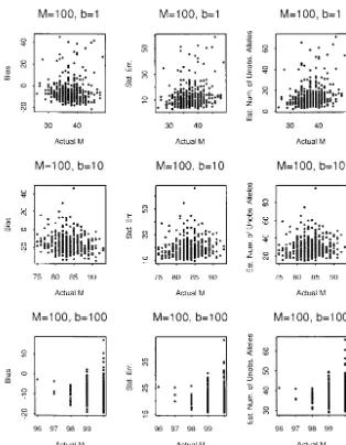
SIMULATION STUDY _{Simulation results under RMM: Since the magnitude}

of CV is reported to be an important effect on perfor-Simulation studies were performed under the

follow-mance, particular configurations ofpi’s are selected to ing three mutation models:

reflect different CV levels. We chose Zipf’s law to specify 1. RMM: Every mutation produces a preexisting type _{allele frequencies because “Zipf’s laws are probability} of allele. It is a reversible process. There is no restric- _{distributions on the positive integers which decay} alge-tion for an allele to mutate to another type as long _{braically. Such laws have been shown empirically to} de-as the mutation rate toward a particular type is not _{scribe . . . the distribution of biological genera and}

zero. _{species” (Chen1980). Its form isp}

iⵑci⫺(1⫹␣)asi→∞. 2. Infinite-allele model (IAM): Each mutation creates _{We select␣ ⫽ 0 so thatp}

i⫽ci⫺1.

a new allele type. _{Under this particular model, suppose the rate for all}

3. Stepwise mutation model (SMM): Each mutation is _{other allele types mutating to a particular type i is␯i.} more likely to change to its adjacent type(s). _{When the population reaches equilibrium, the allele} frequency for alleleiis␯i/␯., where␯.⫽ RMi⫽1␯i. In our Note that, even under the RMM where the number

simulation, we chose␯i ⫽0.0001b/(b ⫹ i) so that the of alleles is set up beforehand, the actual number of

slightly adjusted Zipf’s law is alleles in a population is unknown because of the

evolu-tionary process. For each simulated population, we may

pi⫽ ␯i/␯.⫽

冤

兺

M

j⫽1

(b⫹i)/(b⫹j)

冥

⫺1

⫽c(b⫹i)⫺1_{. (12)}

inter-Figure 1.—The simulation study for the RMM whenM⫽20. Thex-axes are the actual numbers of alleles obtained from the simu-lated populations and they-axes are the quanti-ties described in Equation 11.

The role ofbhere is to adjust the CV of allele

frequen-pi→j⫽

  

␣P(1 ⫺P)j⫺i⫺1 _ifj⬎_i

(1⫺ ␣)P(1 ⫺P)i⫺j⫺1 _ifj⬍_i, cies. The larger the b, the smaller the CV. We choseb

to be 1, 10, and 100 to represent high, medium, and

i.e., the transition probability from typei to typej de-low CV values, respectively.

pends on the absolute value of the size difference (|i⫺

From Figures 1 and 2, we observe that the biases of

j|). If only the size change is concerned, the distribution estimates are all close to 0 when M is small but the

of size change is geometrically distributed. Since estimates exhibit some negative bias when M is large.

This also shows that the number of unobserved alleles

兺

∞

j⬎i

pi→j⫽ ␣, could be very large. We also note that, when CV is large,

the standard error of the estimator is also large.

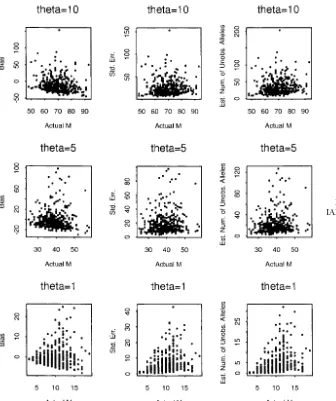
Simulation results under IAM: In the infinite-allele the parameter ␣ is the probability of increasing size case, the parameter␪ ⫽4N␮is selected to be {10, 5, 1}. when a mutation occurs. Hence, if␣ ⬎ 0.5, mutations The results are shown in Figure 3. From the third col- tend to increase the size. The parameter Phas the ef-umn of Figure 3, we see that the difference between fect of determining the magnitude of size change. The the observed and estimated number of alleles increases size change reaches its maximum when P ⫽ 0.5 and as␪values increase. This is reasonable since, when the becomes smaller whenPapproaches its boundaries (0 mutation rate increases, more distinct alleles are ex- or 1).

Although there is no restriction on the size change pected in the population under the IAM.

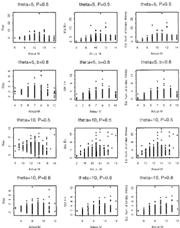
Simulation results under SMM:Under the SMM, we under the model, observations show that each mutation is more likely to change an allele to an adjacent allele. adopted the model proposed byFuandChakraborty

Figure 2.—The simulation study for the RMM whenM⫽100.

when the transition probability greater than that step data from nine populations of honey bee (Apis Mellifera L.) subspecies. The adequacy of two mutation models is less than some critical valueε. The maximum steps

is determined by usually used for microsatellite, IAM and RMM, are tested

by comparing the observed and theoretical number of alleles. The authors claimed that the IAM fits the data

s⫽1⫺ ⫺log10(ε)⫹log10(max{␣, 1⫺ ␣})⫹ log10(P)

log10(1⫺ P) . _{better and argued that the reason may be because the}

majority of the microsatellites they used in the study In our simulation study, we set␣ ⫽0.5 and chose two

contain repeats of several different length motifs. They

Pvalues⫽{0.5, 0.8} and two␪ values⫽{5, 10}. Results

also provided estimates of effective population size are shown in Figure 4. Theεvalue was set to 0.001, so

(2Ne) and mutation rates (␮) for each locus on the basis that the maximum steps forP ⫽0.5 and 0.8 are eight

of some assumptions. We chose the subspeciesTiznitas and four, respectively. Simulation results for different

an example to demonstrate the use of our method. The

␣values are very similar to Figure 4 and are not shown

allele frequencies in Estoup et al.’s data are changed here. On the basis of Figure 4, we observe that, even

to allele counts to fit our need. The data are listed in though we setP⫽ 0.5 and each mutation can change

Table 1. an allele by up to 8 units, the number of alleles observed

Under the IAM, Crow andKimura (1970) derived in the sample is still very limited. Under the same

muta-the expected number of alleles that can be maintained tion rate and sample size, we can observe many more

in a population,MCK, to be alleles under IAM than SMM. As a result, the estimates

are not very different from the observed numbers.

MCK⫽

冮

1

1/2N_e

␪(1⫺ x)␪⫺1_x⫺1_{dx, (13)}

EXAMPLES AND APPLICATIONS

Figure 3.—The simulation study for the IAM.

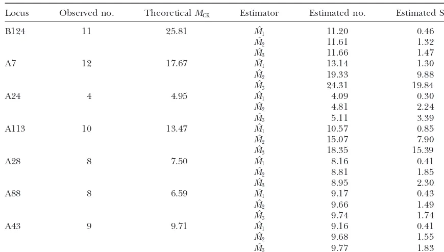
Table 1 together with Equation 13 we can get the theo- relatively small and all the alleles in the data are different (i.e., D ⫽ f1 ⫽ n), we have cˆ⫽ 0 and hence Mˆ ⫽ ∞. retical number of alleles for the population. Table 2

shows the theoretical allele numbers and our three esti- Although in this case we would expect there are many alleles in the population, this estimate is not useful. For mates. The estimated allele numbers are generally close

toMCK. this situation,Chao(1984) derived an estimateMˆlow⫽

D ⫹ f1(f1 ⫺ 1)/2 for the lower bound of M. We use Note that, in some cases, MCK is smaller than the

observed number. This reflects the problem that the this estimate when simulations would give an infinite estimate. In real data, fortunately, this kind of situation two parameters, effective population size and mutation

rate, are generally difficult to estimate and have high is almost impossible.

We also note that when the CV is large, the estimates uncertainty. One advantage of the sample coverage

method is that we do not need to estimate the effective still have a large negative bias. One way to conquer this problem is to use the stabilization technique (Haasand population size and mutation rate before estimating the

allele numbers. Stokes1998) that uses only those alleles appearing less

thanktimes in the sample to obtain the estimates and Besides the direct applications in improving the

esti-mation of gene diversity and characterization of prior then adding alleles having more thankrepresentatives. For example, suppose we haveralleles appearing more distribution of allele frequencies, under SMM, we can

use this information to predict the range of allele sizes thanktimes for a total ofnralleles in the sample. We first use the remaining data (n ⫺ nr) to estimate the as well.

allele number (M⫺r) and then add theralleles back.

Our estimates, therefore, will be Mˆ ⫽ ⫹ r.

DISCUSSION

Since the alleles with high frequencies are not used in estimation, the CV will be reduced significantly. The A drawback of the sample coverage method is that,

Figure4.—The simulation study for the SMM.

removed from the estimation process is that, since they k ⫽ 10 works well (data not shown). We should be careful, however, in applying this technique to real ge-are so abundant, observing them will not provide any

useful information about unseen alleles and hence they netic data, because the variation of frequencies among alleles could be very large. For small samples, removing are not helpful in estimating the total number. The

choice ofkis somewhat arbitrary. Simulations show that alleles with ⬎10 copies from the data may result in an

TABLE 1

The data ofEstoupet al.(1995)

Locus Mutation rate n Allele counts

B124 1.002⫾0.138⫻10⫺3 _{56 f}

1⫽1,f2⫽2,f3⫽2,f4⫽1,f5⫽2,f6⫽1,f12⫽1,f13⫽1

A7 0.686⫾0.138⫻10⫺3 _{46 f}

1⫽4,f2⫽3,f3⫽1,f4⫽1,f5⫽1,f6⫽1,f18⫽1

A24 0.192⫾0.042⫻10⫺3 _{48 f}

1⫽1,f6⫽1,f13⫽1,f28⫽1

A113 0.523⫾0.084⫻10⫺3 _{56 f}

1⫽3,f2⫽3,f5⫽1,f7⫽1,f12⫽1,f23⫽1

A28 0.291⫾0.056⫻10⫺3 _{52 f}

1⫽1,f2⫽2,f3⫽1,f6⫽1,f8⫽1,f12⫽1,f18⫽1

A88 0.256⫾0.051⫻10⫺3 _{54 f}

1⫽1,f2⫽2,f3⫽1,f4⫽1,f6⫽1,f9⫽1,f13⫽1,f14⫽1

A43 0.377⫾0.067⫻10⫺3 _{58 f}

TABLE 2

Results for the data ofEstoupet al.(1995)

Locus Observed no. TheoreticalMCK Estimator Estimated no. Estimated SE

B124 11 25.81 Mˆ1 11.20 0.46

Mˆ2 11.61 1.32

Mˆ₃ 11.66 1.47

A7 12 17.67 Mˆ1 13.14 1.30

Mˆ2 19.33 9.88

Mˆ3 24.31 19.84

A24 4 4.95 Mˆ₁ 4.09 0.30

Mˆ2 4.81 2.24

Mˆ3 5.11 3.39

A113 10 13.47 Mˆ₁ 10.57 0.85

Mˆ2 15.07 7.90

Mˆ3 18.35 15.39

A28 8 7.50 Mˆ₁ 8.16 0.41

Mˆ2 8.81 1.85

Mˆ3 8.95 2.30

A88 8 6.59 Mˆ₁ 9.17 0.43

Mˆ₂ 9.66 1.49

Mˆ3 9.74 1.74

A43 9 9.71 Mˆ1 9.16 0.41

Mˆ₂ 9.68 1.55

Mˆ3 9.77 1.83

MCKassumesNe⫽1617.

unrealistically large estimate because only a very small esting to know the allele numbers for a whole species or how many alleles are shared between subspecies. amount of data is used in the estimation. Hence, we

did not use this technique in Table 2. Chaoet al. (2000) extended the method to this kind

of multipopulation problem in ecology. Further studies Besides these technical problems, some concerns still

need to be addressed. For example, what should we do are needed to adjust their method to population ge-netics.

when some alleles have been reported previously but are

not in the present sample? If there are several samples _{The authors thank anonymous reviewers for their help. This work} available, should we combine them to give a larger sam- was supported in part by National Institutes of Health grant GM 45344. ple or should we use them separately? For the first

prob-lem, assuming there areLalleles we know exist but are

not in our sample, possible solutions are LITERATURE CITED

Bunge, J.,and M. Fitzpatrick, 1993 Estimating the number of 1. Mˆ⬘ ⫽Mˆ ⫹L, or _{species: a review. J. Am. Stat. Assoc.88:364–373.}

Bunge, J., M. FitzpatrickandJ. Handley,1995 Comparison of 3 2. replacenbyn⬘ ⫽n⫹L,D⬘ ⫽D⫹L, andf⬘1 ⫽f1⫹

estimators of the number of species. J. Appl. Stat.22:45–59.

Lto obtainMˆ_⬘, or

Chao, A.,1984 Nonparametric estimation of the number of the 3. sinceMˆ has already estimated the unseen alleles from _{classes in a population. Scand. J. Stat.11:265–270.}

Chao, A.,andS.-M. Lee,1992 Estimating the number of classes via the data, it should already include thoseL alleles.

sample coverage. J. Am. Stat. Assoc.87:210–217. We need only adjust our estimates whenMˆ ⬍ D⫹

Chao, A.,andP. Tsay,1998 A sample coverage approach to

multi-Land set Mˆ⬘ ⫽D⫹L. ple-system estimation with application to census undercount. J.

Am. Stat. Assoc.93:283–293.

For the second problem, besides the method of com- Chao, A., W. H. Hwang, Y. C. ChenandC. Y. Kuo,2000 Estimating the number of shared species in two communities. Stat. Sinica bining data, if the samples are from contemporary

gen-10:227–246.

erations, we can regard them all as a sample from a _{Chen, W.-C.,1980 On the weak form of Zipf’s law. J. Appl. Probab.} capture-recapture experiment. We may use any of sev- 17:611–622.

Crow, J., andM. Kimura,1970 Introduction to Population Genetics eral methods (e.g., Lee and Chao 1994; Norris and

Theory.Harper & Row, New York.

Pollock 1996) for capture-recapture data. Recently _{Darroch, J. N.,and D. Ratcliff, 1958 A note on capture and} ChaoandTsay(1998) proposed a method to estimate recapture estimation. Biometrics36:149–153.

Engen, S., 1978 Stochastic Abundance Model. Chapman & Hall,

M under a multisystem sample scheme that may offer

London.

inter-hierarchical genetic structure and test of the infinite allele and Haas, P.,andL. Stokes,1998 Estimating the number of classes in a finite population. J. Am. Stat. Assoc.93:1475–1487.

stepwise mutation models. Genetics140:679–695.

Esty, W. W.,1982 Confidence intervals for the coverage of low Harris, B.,1968 Statistical inference in the classical occupancy prob-lem: unbiased estimation of the number of classes. J. Am. Stat. coverage samples. Ann. Stat.11:905–912.

Esty, W. W.,1986 The efficiency of Good’s nonparametric coverage Assoc.63:837–847.

Hudson, R. R.,1993 The how and why of generating gene genealo-estimator. Ann. Stat.14:1257–1260.

Feller, W.,1950 An Introduction to Probability Theory and Its Applica- gies, pp. 23–36 inMechanisms of Molecular Evolution, edited byN. TakahataandA. G. Clark.Sinauer Associates, Sunderland, MA. tions.John Wiley and Sons, New York.

Fisher, R., A. CorbetandC. Williams,1943 The relation between Kingman, J. F. C.,1982 The coalescent. Stoch. Proc. Appl.13:235–248.

Lee, S.,andA. Chao,1994 Estimating population-size via sample the number of species and the number of individuals in a random

sample of an animal population. J. Anim. Ecol.12:1257–1260. coverage for closed capture-recapture models. Biometrics50(1):

Fu, Y.-X.,andR. Chakraborty,1998 Simultaneous estimation of 88–97.

all the parameters of a stepwise mutation model. Genetics150: Lewontin, R.,andT. Prout,1956 Estimation of the number of

487–497. different classes in a population. Biometrics12:211–223.

Good, I. J.,1953 On the population frequencies of species and the Norris, J.,andK. Pollock,1996 Nonparametric mle under two estimation of population parameters. Biometrika40:237–264. closed capture recapture models with heterogeneity. Biometrics

Good, I. J.,andG. Toulmin,1956 The number of new species and 52(2): 639–649.

the increase of population coverage when a sample is increased. _{Weir, B. S.,1996 Genetic Data Analysis II.Sinauer Associates,}

Sunder-Biometrika43:45–63. land, MA.

Griffiths, R. C.,1979 A transition density expansion for a