Statistical Analysis of Pathogenicity of Somatic Mutations in Cancer

DOI: 10.1534/genetics.105.044677

Statistical Analysis of Pathogenicity of Somatic Mutations in Cancer

Chris Greenman,*

_{Richard Wooster,* P. Andrew Futreal,* Michael R. Stratton*}

_and

Douglas F. Easton

*Cancer Genome Project, Wellcome Trust Sanger Institute, Cambridge CB10 1SA, United Kingdom,†Section of Cancer Genetics, Institute of Cancer Research, Sutton SM2 5NG, United Kingdom and‡Cancer Research UK Genetic Epidemiology Unit,

Strangeways Research Laboratory, Cambridge CB1 8RN, United Kingdom

Manuscript received April 21, 2005 Accepted for publication June 3, 2006

ABSTRACT

Recent large-scale sequencing studies have revealed that cancer genomes contain variable numbers of somatic point mutations distributed across many genes. These somatic mutations most likely include passen-ger mutations that are not cancer causing and pathogenic driver mutations in cancer genes. Establishing a significant presence of driver mutations in such data sets is of biological interest. Whereas current techniques from phylogeny are applicable to large data sets composed of singly mutated samples, recently exemplified with a p53 mutation database, methods for smaller data sets containing individual samples with multiple mutations need to be developed. By constructing distinct models of both the mutation process and selection pressure upon the cancer samples, exact statistical tests to examine this problem are devised. Tests to examine the significance of selection toward missense, nonsense, and splice site mutations are derived, along with tests assessing variation in selection between functional domains. Maximum-likelihood methods facil-itate parameter estimation, including levels of selection pressure and minimum numbers of pathogenic mu-tations. These methods are illustrated with 25 breast cancers screened across the coding sequences of 518 kinase genes, revealing 90 base substitutions in 71 genes. Significant selection pressure upon truncating mutations was established. Furthermore, an estimated minimum of 29.8 mutations were pathogenic.

R

somatic mutations in human cancers have been started. The primary aim of these screens is to identify the driver mutations in cancer genes that are causally implicated in cancer development (Futrealet al. 2004). Identification of these cancer genes provides major in-sights into the biology of neoplastic change. Moreover, the proteins encoded by some of these mutated cancer genes have recently proven to be tractable targets for new anticancer drug development. However, analysis of the results of genomic screens for somatic mutations can be complicated by a background noise of mutations that confer no clonal growth advantage (passenger muta-tions). For the identification of some driver mutations and cancer genes, the problems caused by background passenger mutations are minor. In a cancer gene that is frequently involved in cancer development, the somatic mutation frequency per nucleotide of coding sequence in a set of cancer samples is clearly higher than in other genes and is often characterized by distinctive patterns of mutation type and/or position. For example, mutations observed in BRAF mostly cluster in exons 11 and 15, with a large subset of these consisting of the single mutation V600E (Davieset al. 2002). However, such features will

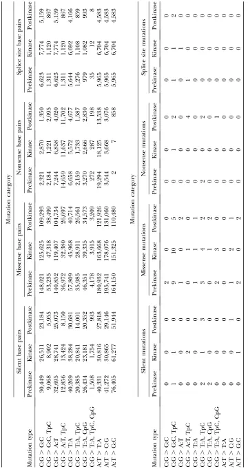
not easily be detected in cancer genes that are infre-quently involved in cancer causation, unless very large numbers of cancer samples are analyzed. For example, in a recent screen of 518 kinase genes of 25 breast cancers (Stephenset al. 2005), 90 base substitutions were dis-covered in 71 genes. The number of mutations per gene was highly correlated with the coding sequence length, and no gene with a clear elevation in its mutation rate per coding nucleotide presented itself as a candidate cancer gene. Since 14 of these mutations were silent and hence likely to be passenger mutations (see Table 1) this opens the question of determining whether any of the re-maining 76 mutations are pathogenic, which would provide evidence that some of the 71 mutated genes are involved in the formation of cancer.

A similar problem was considered by Yang et al. (2003). Phylogenetic techniques from evolution ana-lyses were adapted to analyze a large database containing p53 mutations, and missense and nonsense mutations were successfully shown to have different effects across distinct functional domains of biological interest. How-ever, this data set is marked by characteristics that distinguish it from the protein kinase data set provided in Stephenset al. (2005), implying that alternative ana-lyses may be more appropriate for the latter. Samples in the p53 data set typically contain a single mutation and were modeled as such in Yanget al. (2003). This is not the case for the protein kinase data set, where some 1_{Corresponding author:Cancer Genome Project, Wellcome Trust Sanger}

Institute, Wellcome Trust Genome Campus, Hinxton, Cambridge CB10 1SA, United Kingdom. E-mail: [email protected]

cancers with mutator phenotypes contain several muta-tions, which need to be modeled accordingly. The pro-tein kinase data set is of moderate size, meaning exact tests are more desirable than the asymptotic likelihood-ratio tests applied to the large p53 data set.

Current methods (Yanget al. 2003) can establish the existence of pathogenic mutations, without indicating the proportion of nonsynonymous mutations that are pathogenic rather than passenger in nature. This param-eter is a desirable quantity as it is indicative of the proportion of mutated genes that are implicated in the development of oncogenesis. The methods described below incorporate these differences into the modeling techniques.

Finally we note that current methods (Yang et al. 2003) incorporate selection toward certain mutation types as multiplicative weighting factors in codon sub-stitution models. We present a method whereby selec-tion is explicitly described as a process separate from mutation, from which the full model of observables can be constructed accordingly. This allows any model of selection in cancer to be developed and explored.

In this article we use a similar approach to phylogenetic methods to evaluate the evidence that the observed data set contains pathogenic mutations. The basic principle behind this approach is that silent (synonymous) so-matic mutations are passenger mutations. Although a minority of apparently synonymous mutations may en-code exonic splice enhancers or other cryptic elements that affect the translated product of a DNA sequence, in general this assumption is likely to be correct. The set of silent mutations can therefore be used as a control group to estimate the number of nonsilent mutations that would be expected to occur by chance, under the null hypothesis of no association between mutations and cancer development. Tests of significance can then be derived by comparing the observed number of non-silent (nonsynonymous) mutations to the expected number. It is also possible to derive estimates of the minimum proportion of mutations likely to be patho-genic. We also show that there is a strong analogy with standard analyses of epidemiological case–control or cohort studies to evaluate risk factors.

To develop the approach, we consider an experiment in which a number of tumors are screened through a particular coding sequence. Suppose thatlsilent muta-tions and n nonsilent mutations are observed, with t¼l1n mutations in total. We further assume that there areTpossible mutations across the sequence (T is three times the length of the sequence), of whichL are silent and N are nonsilent. Thus a randomly po-sitioned mutation will be silent with probability p0¼

L=T. If tumor samples exhibit no preference toward either silent or nonsilent mutations, thenp0 also

rep-resents the probability that a randomly chosen mutation from a tumor sample will be silent. The odds ratio n=l3p0=ð1p0Þ is a measure of the strength of the

association or selection toward nonsilent mutations. Values greater than unity would indicate positive selec-tion (that is, nonsilent mutaselec-tions occurring more often than would be expected by chance and, therefore, to some degree related to cancer development), while values less than unity would indicate negative selection (nonsilent mutations occurring less often than ex-pected, perhaps because they result in cell death). However, any deviation from unity may be due to the random nature of mutation rather than to any un-derlying positive or negative selection by cancer. Alter-natively, if any of the N nonsilent mutations either promote or inhibit the development of cancer, the probabilitypthat a randomly chosen mutation observed in cancer is silent may differ fromp0. These two scenarios

can be summarized by null and alternative hypotheses H0:p¼p0 and H1:p 6¼p0. Note thatpis unobservable,

so inference statistics are required to compare the hy-potheses. The significance level of a suitable statistic, such as the odds ratio, would enable such a comparison. To obtain this, the expected distribution of the odds ratio under the null hypothesis is required. If we con-dition upon the total number of observed mutationst we note that under the null hypothesis H0the number of

silent mutationslwould be drawn from a Binomial (t,p0)

distribution. The expected distribution can then be estimated by simulatinglfrom this distribution and cal-culating numerous odds ratios (p0is a function of DNA

sequence and so fixed throughout). Comparing the ob-served odds ratio to this distribution will then provide a significance level. This will help determine whether any of the observed nonsilent mutations are likely to have contributed to oncogenesis in the sampled tumors.

must be adjusted for. This is accomplished most simply by considering each mutation type as a separate stratum. The mutation rate may depend not only on the mu-tated base but also on the neighboring sequence. For example, C:G . T:A mutations occur at an increased rate due to deamination of cytosine at CpG dinucleo-tides. In principle, such neighborhood effects can be handled by introducing larger numbers of strata, al-though the required number of strata may be large (for example, if all combinations of bases on both sides of the mutated base are considered, there are 192 possible mutation types). Such finer stratification will reduce the risk of bias but will also reduce power. For example, a C:G . G:C mutation at the central nucleotide of an ApGpG trinucleotide cannot be silent. Any selection pressure on such mutations will elevate the mutation rate of this stratum. However, this cannot be distin-guished formally from an inherently different mutation rate at these sequences, so such mutations are un-informative. In practice, a compromise between repre-sentative stratification and statistical power is required. Deamination at CpG dinucleotides is well established, and a strong C:G.{T:A, A:T, or G:C} mutation rate at TpC dinucleotides was observed in Stephens et al. (2005). For our main analyses, we have used the 11 strata given in Table 1.

The degree of selection by cancer upon specific muta-tions may depend on the type of amino acid change adopted by the protein. In particular, nonsense and splice site mutations can lead to a truncated or reduced protein, respectively, or indeed to total absence of pro-tein through nonsense-mediated decay, which may re-move domains of functional importance. If any such mutations occur in the presence of loss of heterozygosity (LOH) on the homologous chromosome, function will be lost. This is the mechanism by which many tumor suppressor genes are involved in carcinogenesis. For example, the mutation data set of the RB1 tumor sup-pressor gene examined in Valverdeet al. (2005) con-tains more nonsense and splice mutations than are typical for the pattern of mutations observed in hered-itary diseases. Conversely, a dominant change in func-tion is more likely to be achieved through missense mutations. Furthermore, proteins containing multiple domains of functional necessity are less likely to tolerate deletions induced by nonsense and splice variants, as exemplified by the p53 gene, where most of the re-corded variants are missense, as can be found in the data-base described by Be´ roud and Soussi (2003). These potential differences in selection by cancer can be in-corporated by separating nonsilent mutations into mis-sense, nonmis-sense, and splice site categories.

The nucleotides most likely to induce splice variants under mutation are 1, 2, or 5 bp 39to an exon or 1 or 2 bp 59to an exon. Although other nucleotides may be sources of splice variants under mutation, they have been ignored in this analysis.

This idea may be extended to consider separately different types of amino acid substitutions. For exam-ple, conservative and nonconservative changes could be differentiated. Alternatively, the heterogeneity of var-iants could be distinguished to reflect the idea that pathogenic homozygous variants are likely to occur in recessive cancer genes, whereas pathogenic heterozy-gous variants will occur in dominant cancer genes.

The functional domains of the genes under in-vestigation may also be subject to different selection pressures. For example, tumor cells may not tolerate mutations within some highly conserved regions, possi-bly inducing apoptosis, which will be selected against by cancer. Alternatively, mutations in functional domains key to mitotic pathways may enhance the clonal growth rate, such as within the kinase domains of certain pro-tein kinases. These mutations will be under positive selection pressure by cancer. Establishing differences in selection across distinct functional domains within the screened genes thus becomes a question of biological interest.

This article is organized as follows. The next section introduces the Poisson processes used to model the random nature of mutations under no selection pres-sure. To describe the pattern of mutations observed in tumor samples, the subsequent section models the selec-tion pressure of cancer upon mutaselec-tions, from which methods to estimate the numbers of pathogenic muta-tions are introduced. Likelihood-ratio and score statistics are then developed to assess whether selection pressure upon the screened genome exists and hence whether a subset of the observed mutations is implicated in the development of cancer. Next, these methods are adapted to test for variation in selection across different func-tional domains. Finally, these techniques are illustrated and discussed with the breast cancer data set of Stephens et al. (2005).

MODELING MUTATIONS

Various models of the mutation process have been defined and explored, frequently to model the

evolu-tionary development of species (see Goldman and

Suppose we haveJtumor samples to analyze. Suppose furthermore that tumor sample j has undergone mj

mitoses and that, at therth mitosis, the number of muta-tions in the screened coding sequence (CDS) of typekis a Possion process with raterr

jk, where the mutation typek

represents 1 of 11 strata indicated in Table 1. The num-ber of mitoses and mutation rates may vary among sam-ples, and the mutation rates may vary between mitoses. It is assumed throughout that these intensities are small and that all processes are independent. Note that these mutation intensities are unobservable. Furthermore, although these are of biological interest, the main mo-tivation of the present analysis is to evaluate the evi-dence for pathogenicity. In the current context, the mutation intensities are nuisance parameters to be elim-inated by estimation or conditioning.

For each mutation typekwe calculate the number of base pairs in the CDS that can give rise to silent, mis-sense, nonmis-sense, or splice mutations. These counts are denotedLk;Mk;Nk, andSk, respectively, with totalsTk¼

Lk1Mk1Nk1Sk. These observables can be calculated

precisely from the sequence of DNA in the region screened, available from any database containing the human genome sequence, and the genetic code. The values for the kinase data set of Stephens et al. (2005) are provided in the top half of Table 1.

Some genes may have multiple transcripts, possibly out of frame, making such counts ambiguous. In such cases average counts weighted by protein frequency would be appropriate, if possible. However, for applica-tion to the protein kinase genes in Stephens et al. (2005), multiple transcripts varied little and no frame-shifts were observed, so only the longest transcript was used in application of these methods.

Single-nucleotide polymorphisms (SNPs) in the sam-ples will result in some differences between the sample CDSs and a database reference CDS. These are normally detected when wild-type samples are screened against the cancers to distinguish SNPs from somatic mutations. In principle, values ofLk,Mk, Nk, and Skcould be

ad-justed to take account of these SNPs. However, since they typically occur at an average frequency of about one every kilobase, errors involved in using the reference sequence were assumed negligible.

The aim of this article is to distinguish pathogenic mutations from passenger ones. It is thus natural to divide each of missense, nonsense, and splice mutations into two groups, those associated with cancer (driver or pathogenic) and those not associated with the growth rate of cells (passenger or neutral). As such, we parti-tion the countsMk¼Mkc1M

c

k,Nk¼Nkc1N

c

k, andSk¼

Sc

k1S

c

k, where superscript c indicates a count across

bases pathogenic under mutation, and c indicates

counts across bases neutral to cancer. Although only the totalsMk,Nk, andSkcan be observed, the division of

counts into pathogenic and neutral counts serves the problem twofold. First, selection pressure induced by

cancer will apply only to the pathogenically mutable bases. Second, this will allow us to estimate the number of pathogenic mutations.

Suppose that ljk, mjk¼mcjk1mjkc, njk ¼njkc 1ncjk, and

sjk¼sjkc 1sjkc are the numbers of silent, missense,

non-sense, and splice site mutations actually observed in samplej. Again, the missense, nonsense, and splice site counts are partitioned into pathogenic or passenger mu-tations. The total counts are denoted tjk ¼ljk1mjk1

njk1sjk. Then assuming that mutations are

indepen-dent random events, the counts ljk;mjkc;m c jk;n

c jk;n

c jk;s

c jk,

and sc

jk will be drawn from independent Poisson

dis-tributions with expectations Lkrjk;Mkcrjk;Mkcrjk;Nkcrjk;

Nc

krjk;Skcrjk, and Skcrjk, respectively, where rjk ¼ P

rr

r jk

represents the overall intensity across all mitoses of samplejfor mutation typek. Although each mutation may change Lk;Mkc;Mkc;Nkc;Nkc;Skc, or Skc slightly, the

total number of mutations is typically small enough that these sizes can be regarded as fixed. For example, the breast kinase screen of Stephenset al. (2005) detected only 90 base substitutions out of 3.23107_{bp screened.}

In the absence of any selection pressure, the proba-bility of observing a given set of mutations in samplej then takes the form of the following product of Poisson distributions:

Prðfljk;mjkc;mcjk;ncjk;njkc;sjkc;scjkgk¼1;...;11Þ

¼Y

k

eTkrjk_rtjk jk

LkljkðMkcÞ mc

jkð_Mc kÞ

mc jkð_Nc

kÞ nc

jkð_Nc kÞ

nc jkð_Sc

kÞ sc

jkð_Sc kÞ

sc jk

ljk!mjkc!mjkc!njkc!njkc!sjkc!scjk!

:

ð1Þ

Note that the ratios a_jk ¼r_jk=P_k9r_jk9 represent the probability that a random mutation is of typek. These values are commonly referred to as the mutation spectra.

MODELING SELECTION

expression levels may vary between samples, for exam-ple. For these reasons, it is natural to model the devel-opment of cancer for a given mutation set stochastically rather than deterministically.

If Cj denotes the event that a given cell lineage j

develops cancer, the distribution of observed mutations can be resolved through Bayes’ theorem into the fol-lowing product,

Prðfljk;mjkc;mjkc;ncjk;njkc;scjk;scjkgk¼1;...;11jCjÞ

}Prðfljk;mjkc;mjkc;njkc;ncjk;sjkc;sjkcgk¼1;...;11Þ 3PrðCjj fljk;mjkc;mjkc;ncjk;njkc;scjk;scjkgk¼1;...;11Þ: The final term PrðCjj fljk;mjkc;m

c jk;n

c jk;n

c jk;s

c jk;s

c

jkgk¼1;...;11Þ

models the probability that a DNA sample with the given set of mutations across the region screened will be cancerous.

The form of these latter terms will depend on the assumed model of cancer. Some models, for example, assume that a fixed number of mutations are observed. This is a general fixed parameter in Littleand Wright (2003). The work of Yanget al. (2003) fit numerous models to data arising from experiments where one or a few genes are screened across numerous samples, ex-emplified by their analysis upon a p53 mutation data set. However, the typical data set considered here contains the results of a screen across several genes in relatively few tumor samples, such as that described in Stephens et al. (2005). As such, we assume that for all samples, each additional pathogenic mutation of a given cate-gory confers the same relative increase in the probability of developing cancer. Although this may not be strictly true, it provides an intuitive model for developing tests and estimates. The final term will thus be of the form,

PrðCjj flkj;mkjc;mkjc;nkjc;nkjc;sckj;skjcgk¼1;...;11Þ}h

mc j_mncj_nsjc_;

ð2Þ

wheremc

j ¼

P

km

c jk;n

c

j ¼

P

kn

c jk, ands

c

j ¼

P ks

c

jkdenote

the total numbers of pathogenic missense, nonsense, and splice mutations in samplej, respectively.

We note that this probability is independent of muta-tion counts within each mutamuta-tion type,k. This may be expected, as the likelihood of developing cancer is likely to depend upon the category of amino acid change (i.e., missense, nonsense, or splice) rather than the type of source mutation,k.

The termsh;m, andn represent the relative change in probability of developing a tumor conferred by a pathogenic missense, nonsense, or splice mutation, respectively. Values greater than unity indicate an in-crease in this likelihood, whereas values less than unity represent a decrease. These terms are analogous to rate ratios or relative risks in epidemiology, where the mu-tations are analogous to exposures. The resulting likeli-hood is then of the form

Prðfljk;mjkc;mcjk;ncjk;njkc;sjkc;scjkgk¼1;...;11jCjÞ

¼Y

k

erjkðLk1hMkc1mN c k1nS

c k1M

c k1N

c k1S

c kÞ

3rtjk_jkL

ljk kðhMkcÞ

mc jk_ðmNc

kÞ nc

jk_ðnSc kÞ

sc jk_ðMc

kÞ mc

jk_ðNc kÞ

nc jk_ðSc

kÞ nc

jk

ljk!mjkc!mjkc!njkc!ncjk!sjkc!sjkc!

:

ð3Þ

This is equivalent to a product of independent Pois-son distributions where ljk;mjkc;m

c jk;n

c jk;n

c jk;s

c

jk, and s c jk

have intensities given by r_jkLk;rjkhMkc;rjkMkc;rjkmNkc;

r_jkNc

k;rjknSkc, andrjkSkc, respectively. Iflk;mk;nk, and sk

denote the total number of silent, missense, nonsense, and splice variants across all samples, we have lk¼ P

jljk;mk¼ P

jðm c

jk1m

c

jkÞ;nk¼

P jðn

c

jk1n

c

jkÞ, and sk¼ P

jðs c

jk1sjkcÞ. As mutations are independent events, the

counts lk;mk;nk, and sk will also follow independent

Poisson distributions, with intensities given byr_kLk;rk

ðhMc

k1MkcÞ;rkðmNkc1NkcÞ, and rkðnSkc1SkcÞ,

respec-tively, wherer_k¼P_jr_jk. This can be summarized by Prðflk;mk;nk;skgk¼1;...;11j fCjgj¼1;...;JÞ

¼Y

k

erkðLk1Mkfk1Nkck1SkzkÞ_rtk k

3L

lk

kðMkfkÞmkðNkckÞnkðSkzkÞsk

lk!mk!nk!sk!

; ð4Þ

wheref_k¼ ðhMc

k1M

c

kÞ=Mk,ck¼ ðmNkc1N

c

kÞ=Nk, and

z_k¼ ðnSc

k1S

c

kÞ=Skare the rate ratios and represent

selec-tion pressures. Valuesf_k;c_k;z_k.1 increase the probabil-ity of observing pathogenic mutations and thus represent positive selection pressure, whereasf_k;c_k;z_k,1 indicate negative selection pressure.

It is worth observing that although the parametersh, m, andn, used to define the probability that a cell lineage adopts cancer (Equation 2), are independent of muta-tion typek, differences in the proportions of potentially pathogenic mutations (i.e., Mc

k=Mk, Nkc=Nk, or Skc=Sk),

could still lead to selection pressures f_k;c_k;z_k that depend uponk. We also note that, in the present con-text, these parameters are assumed to be the same for all mutations of each type. In practice this may not be true, in which case they can be regarded as a representative ‘‘average’’ effect. Later, we consider approaches to eval-uating variation in these parameters, for example, by domain.

ESTIMATING THE NUMBER OF PATHOGENIC MUTATIONS

One question that naturally arises is how to estimate the proportions of observed mutations that are actually pathogenic. These are denotedrm¼mkc=mk;rn¼nkc=nk,

and rs¼skc=sk for missense, nonsense, and splice

var-iants, respectively, which can be estimated by taking the ratio of the relevant rates from Equation 3. This gives ˆ

rm¼hMkc=ðhM c

k1M

c

kÞ ¼1M

c

mutations, with similar estimates ˆrn¼1Nkc=ðckNkÞ

and ˆrs¼1Skc=ðzkSkÞfor nonsense and splice site

muta-tions. In practice, of course these cannot be determined since the countsMc

k;Nkc, andSkcare unobservable.

How-ever, in the limit whereMc

k/Mk;Nkc/Nk, andSkc/Sk

(i.e., most base pairs are neutral under mutation) and assuming positive selection, these probabilities con-verge to 11=f_k;11=c_k, and 11=z_k, respectively. Since these expressions are also the fractions of muta-tions that occur in excess of expectation under no selection, this is perhaps the natural answer to the ques-tion as to what fracques-tion of mutaques-tions can be attributed to the cancer. However, because Mc

k#Mk;Nkc#Nk, and

Sc

k#Sk, these expressions are lower bounds on the

portion of mutations actually involved in the disease pro-cess. At the opposite extreme one might haveMc

k/0;

Nc

k/0, and Skc/0, implying that all nonsilent

muta-tions are (more weakly) pathogenic. More strictly, there-fore, provided selection pressure is positive, the estimated proportions of missense, nonsense, and splice site muta-tions that are pathogenic are described by the inequalities

11=f_k#rˆm#1; 11=c_k#rˆn#1; 11=z_k#rˆs#1:

These ranges reflect the idea that one cannot distin-guish between a small number of mutations conferring strong selection and a larger number of mutations conferring weak selection.

In the case of negative selection, no information upon rm;rn, orrscan be provided. However, sinceh;m;n.0,

lower bounds for any negative selection pressuresf_k. Mc

k=Mk;ck.Nkc=Nk, and zk.Skc=Sk result. Therefore,

under negative selection pressure,f_k;c_k, andz_kprovide upper bounds on the proportion of base pairs that are selected against by cancer.

TESTS OF SELECTION

So far we have developed a model (summarized by Equation 4) for mutations across a section of screened

genome, which incorporates selection pressures. The observable parameters include the silent, missense, non-sense, and splice site mutation countslk;mk;nk, andsk,

along with base pair counts Lk;Mk;Nk, andSk,

respec-tively. The unobservable parameters include the selec-tion pressures, represented in the model by the terms fk,ck, andzk, and the parametersrk, which represent a

mutation rate for each typek.

The principal aim of the analysis is to examine evi-dence for selection. That is, determine if any offk,ck,

andz_kare distinct from unity, indicating that a subset of the point mutations detected across the screened ge-nome are related to the genesis of cancer in the sampled tumors. Unfortunately the selection pressures cannot be directly measured, and we have to rely on the ob-servables to derive estimates, denoted f^_k, c^_k, and^z_k. Although these estimates may differ from unity, the pop-ulation valuesfk,ck, andzkcould still be unity,

differ-ences arising due to natural random fluctuation in the observed mutation counts, rather than a genuine un-derlying effect. This is an inference problem, typically examined by considering two alternatives, the null hy-pothesis (neutral selection) and an alternative hypoth-esis (selection by cancer), where a significance value provides a measure of the strength of evidence support-ing the alternative hypothesis.

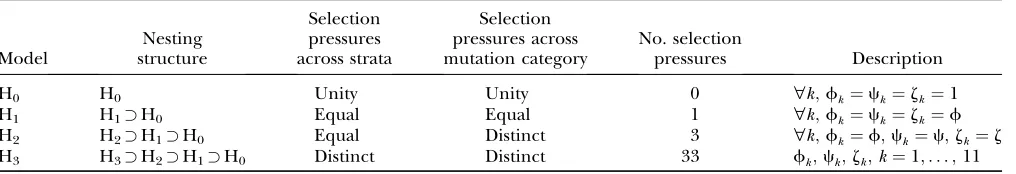
For the problem in hand, there are many possible alternative hypotheses, and it is desirable to know which one is most likely. We can express the possible scenarios in terms of the four hypotheses described in Table 2. H0

is the global null hypothesis of no selection pressure. H3

is the most general alternative, allowing for positive or negative selection pressures, heterogeneous across mu-tation types. The alternatives H1and H2assume that the

selection pressures, as measured byf,c, andz, are com-mon across mutation types. These reflect the notion that different mutation types are equally likely to be associated with disease. H1 differs from H2in further

assuming that the selection pressures for missense, nonsense, and splice site mutations are equal.

To develop estimates of the selection pressures and statistical tests to evaluate the above hypotheses, we must TABLE 2

Properties of the four hypotheses H0, H1, H2, and H3

Model

Nesting structure

Selection pressures across strata

Selection pressures across mutation category

No. selection

pressures Description

H0 H0 Unity Unity 0 "k;fk¼ck¼zk¼1

H1 H1H0 Equal Equal 1 "k;fk¼ck¼zk¼f

H2 H2H1H0 Equal Distinct 3 "k;fk¼f;ck¼c;zk¼z

H3 H3H2H1H0 Distinct Distinct 33 fk;ck;zk;k¼1;. . .;11

first eliminate the unknown nuisance parametersr_k. A natural approach is to argue conditionally on the total number of mutations tk of each type. These are the

minimal sufficient statistics for r_k, which are conse-quently eliminated. This leads (from Equation 4) to a product of multinomial distributions:

Prðflk;mk;nk;skgk¼1;...;11j ftkgk¼1;...;11Þ

¼Y

k

tk!

lk!mk!nk!sk!

Llk

kðMkfkÞmkðNkckÞnkðSkzkÞsk

ðLk1Mkfk1Nkck1SkzkÞtk

: ð5Þ

Again, it is interesting to note that there is a strong analogy with the analysis of cohort studies in epidemi-ology. The mutation types are equivalent to different strata in a cohort analysis, while the termsLk,Mk,Nk, and

Skare equivalent to the ‘‘person years’’ at risk.

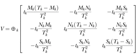
Several different tests for selection can now be devel-oped, on the basis of the possible alternative hypothe-ses. Likelihood methods provide a natural framework for hypothesis tests, and maximum-likelihood estima-tion can also be used to estimate the various parameters. One standard approach to hypothesis testing is to use a likelihood-ratio test (LRT), on the basis of the ratio of the maximum likelihoods under the two hypotheses. In large samples LRT statistics are distributed, asymp-totically, as chi-square distributions, provided that the hypotheses are nested. However, the likelihood ratio may not be analytically tractable, in which case numer-ical methods may need to be applied. An alternative class of test statistics is score tests, based on the first derivativeUof the log-likelihood at the null. The score statistic is of the formV¼UT_V1_{U, whereVis the}

co-variance ofU, and this also has an asymptotic chi-square distribution, provided that the null hypothesis is nested in the alternative hypothesis. The LRT and score test also have similar efficiency (Coxand Hinkley1974). If the data set is small (e.g., Stephenset al. 2005), or hy-potheses are not nested, the chi-square approximations may not be reliable. In these cases, the significance levels may be estimated by simulation, using permuta-tion arguments in which mutapermuta-tions are randomly per-muted among tumors. Permutation arguments could be applied to LRTs but are more easily applied to score tests since they can often be computed without iteration. Fur-ther details of these methods can be found in Sorensen and Gianola(2002).

These statistics can be used to test the null hypothesis H0against alternatives H1, H2, or H3. Which test is to be

preferred depends on the likely alternative hypothesis and comes down to a trade-off between generality of the alternative and number of unknown parameters in the test (respectively 1, 3, and 33). In general, our prefer-ence is for a primary test of H0vs. H2rather than H0vs.

H1, since this reflects the fact that missense, nonsense,

and splice mutations are likely to behave differently. This is reinforced by results of Yanget al. (2003), where

differences between missense and nonsense selection pressures were observed. A test to compare H1 vs. H2

would also help resolve this issue. The more general test of H0vs. H3would be expected to lack power given the

large number of parameters, unless there is strong reason to suspect a marked tendency for mutations of a particular type to be pathogenic. One would then want to conduct a separate test of H2 vs. H3 to evaluate

whether there is evidence of heterogeneity in selection pressure across mutation types.

We note that the hypotheses H0, H1, H2, and H3are

nested, as indicated in Table 2. The LRT comparing any pair of hypotheses then has a standard chi-square dis-tribution, provided data sets are of sufficient size. The likelihoods used in this ratio are derived from the con-ditional likelihood in Equation 5, maximized with re-spect to all free parameters (selection pressures) within each hypothesis. The number of degrees of freedom required to implement the LRT is simply the difference between the numbers of free parameters for each hy-pothesis, as indicated in Table 2. However, for data sets of moderate size, the resulting significance levels may not be accurate, so exact score tests can be derived to provide more reliable information.

The score test for comparison of H0vs. H2is based on

the first derivativesUof the log-likelihood with respect to the selection pressuresf,c, andz, evaluated at the null hypothesisf¼c¼z¼1. Then using Equation 5, this leads to a test statistic of the form V¼UT_V1_U,

where

U ¼ X

k

ðmktkMk=TkÞ; X

k

ðnktkNk=TkÞ;

X

k

ðsktkSk=TkÞ

;

and covariance

V ¼

P

k

tkM

kðTkMkÞ

Tk2

P k

tkMkNk

Tk2

P k

tkMkSk

Tk2

P k

tk

NkMk

T2

k

P

k

tk

NkðTkNkÞ

T2

k

P k

tk

NkSk

T2

k

P k

tkSkMk

Tk2

P k

tkSkNk

Tk2

P

k

tkSk ðTkSkÞ

Tk2

2 6 6 6 6 6 6 6 6 6 4

3 7 7 7 7 7 7 7 7 7 5

:

In the epidemiological literature this is just the Mantel–Haenszel test for cohort studies. The terms

P

ktkMk=Tk;PktkNk=Tk, and PktkSk=Tk can be

thought of as the expected numbers of missense, non-sense, and splice site mutations under the null hypoth-esis of no selection, given the total number of mutations observed. Exact significance levels can be computed by simulating the null distribution of the test statistic, randomly reallocating thetkmutations of typekto the

A similar test for H0 vs. H1 can be constructed by

combining missense, nonsense, and splice site muta-tions into a single category for each mutation type.

For the more general test of H0vs. H3,

U ¼ fðmktkMk=TkÞ;ðnktkNk=TkÞ;ðsktkSk=TkÞgk¼1;...;11

and

V¼4_k tk

MkðTkMkÞ

T_k2 tk MkNk

T_k2 tk MkSk

T_k2

tk

NkMk

T_k2 tk

NkðTkNkÞ

T_k2 tk NkSk

T_k2

tk

SkMk

T_k2 tk SkNk

T_k2 tk

SkðTkSkÞ

T_k2

2 6 6 6 6 6 6 6 6 4

3 7 7 7 7 7 7 7 7 5 :

For this comparison the relevant likelihoods can be maximized without iteration, so that exact tests based on a LRT are also straightforward. The likelihood-ratio statistic in this case can be obtained by maximizing the conditional likelihood in Equation 5 with respect to all the selection pressures:

LRðflk;mk;nk;skgk¼1;...;11Þ

¼Y

k

ðlk=tkÞlkðmk=tkÞmkðnk=tkÞnkðsk=tkÞsk

ðLk=TkÞlkðMk=TkÞmkðNk=TkÞnkðSk=TkÞsk

:

It is also desirable to derive comparisons between the different alternatives. The most straightforward test for H1vs. H3or H2vs. H3is a likelihood-ratio test. In this

case there is no straightforward exact test and numeri-cal iterative methods are required (only H2vs. H3was

implemented in application). However, an exact test for H1vs. H2can be achieved with the methods described in

functional domains below. Viabilities of likelihood-ratio and score tests for comparisons between the dif-ferent hypotheses are summarized in Table 3.

We note that the tests described above can be applied individually to missense, nonsense, or splice site mu-tations. For example, one may want to examine the

sig-nificance of the selection pressure upon nonsense mutations c_k, irrespective of the missense and splice site selection pressures f_kandz_k. That is, test null hy-pothesis H0:ck¼1 against H1:ck6¼1. This can be

achieved by simply removing all terms involving mk;

Mk;sk;Sk from the expressions above, redefining the

totals tk¼lk1nk;Tk¼Lk1Nk in terms of silent and

nonsense counts only, and proceeding as before. Tests specific to missense or splice variants are achieved similarly.

Parameter estimation under the various alternative hypotheses can be found by implementing maximum-likelihood methods. Under the most general model H3,

these are given (from Equation 5) by the usual odds ratios:

f^_k¼mk

lk

Lk

Mk

; c^_k¼nk

lk

Lk

Nk

; ^z_k¼sk

lk

Lk

Sk

:

Under the more restrictive models H1 and H2,

maximum-likelihood estimates can be obtained only iteratively. However, from Equation 4, countslk;mk;nk,

andskare Poisson with meansrkLk,rkMkfk,rkNkck, and

rkSkzk, respectively. Thus estimation for the various

un-known parameters, including the nuisance parameters, can be obtained by implementing Poisson regression with a log link function in one of the standard packages capable of fitting generalized linear models (for exam-ple, Matlab, Stata, or S plus). The terms log(Lk), log(Mk),

log(Nk), and log(Sk) are handled as offsets in the

anal-ysis. Confidence intervals for the parameters, based on standard asymptotic arguments, are also produced by these routines.

The terms ˆmc

k¼mkð11=f^kÞ;nˆck¼nkð11=c^kÞ, and

ˆ sc

k¼skð11=^zkÞ estimate the minimum number of

pathogenic missense, nonsense, and splice site muta-tions, respectively (assuming positive selection pres-sure). That is, they estimate the minimum number of mutations attributable to the disease process. It may be preferable to replace f^k, c^k, and^zk by common

estimates across mutation types (i.e., assume hypothesis H2) if there is no evidence of heterogeneity.

Although the main interest is in the selection param-eters associating mutation with disease, it is also possible to make simultaneous inferences about the mutation spectra ak¼rk=

P

krk. The maximum-likelihood

esti-mates for ˆr_k from Equation 4 are given by ˆr_k¼

tk=ðLk1Mkf^k1Nkc^k1Sk^zkÞ. These mutation rates are

generated naturally in the Poisson regression analyses. The estimates ˆa_k¼ˆr_k=P_krˆ_kcan then be calculated for any of the alternative hypotheses.

Finally, we observe that a parameter of common bio-logical interest is the probability that a mutation is silent. By writing PrðSilentÞ ¼P_kPrðSilentjkÞPrðkÞ, this can readily be estimated by

PˆrðSilentÞ ¼X

k

Lkaˆk

Lk1Mkf^k1Nkc^k1Sk^zk

: ð6Þ

TABLE 3

Preferential comparisons between hypotheses H0, H1, H2, and H3

H0 H1 H2 H3

H0 — Score Score Score, LRT

H1 Score — Scorea LRTb

H2 Score Scorea — LRTb

H3 Score, LRT LRTb LRTb —

All comparisons can be implemented as exact tests. a

The more general score statistic described in the domains section is required.

b

Note that this estimated probability is a function of DNA sequence, selection pressure, and mutation spectra, under the alternative hypotheses. This will correct for any biases arising from the heuristic ratioP_klk=Pktk.

FUNCTIONAL DOMAINS

The above models can be extended to evaluate the possibility of differential selection according to addi-tional covariates. This might include, specifically, func-tional domains or subsets of genes. Suppose that the DNA sequence screened is divided intoHdomains of interest. Suppose furthermore that we are interested in detecting differential selection toward missense muta-tions between these domains. Nonsense and splice site variants are (for the moment) ignored. The rate of silent mutations per nucleotide will be constant across these domains by the hypothesis of neutral selection. We are therefore interested only in missense mutations throughout these domains. By defining domain-specific selection pressures, mutation counts, and base pair counts, the density Prðfmkhgk¼1;...;11;h¼1;...;HÞ can be

ex-pressed as the following product of Poisson distributions:

Prðfmkhgk¼1;...;11;h¼1;...;HÞ ¼ Y

kh

ðr_kMkhfkhÞmkh

mkh!

erkMkhfkh_:

This term is essentially Equation 4 restricted to just missense mutations, where all terms exceptr_khave an additional subscript h referring to the domain. The mutation ratesr_kare assumed constant across domains, implying that significant differences in mutation counts between domains are due to variation in selection pressure alone.

Assuming independence of mutations between do-mains, the total number of mutations across all domains for each mutation typek will also have a Poisson dis-tribution, with the rate equal to the sum of individual rates across domains, so that

Prðfmkgk¼1;...;11Þ ¼

Y

k

ðr_kP_hMkhfkhÞmk

mk!

erk P

hMkhfkh:

As we wish to compare domain-specific selection pressures irrespective of the overall selection pressure, it is natural to consider the distribution of the domain-and type-specific mutation counts, conditional on the total type-specific counts:

Prðfmkhgk¼1;...;11;h¼1;...;Hj fmkgk¼1;...;11Þ

¼Y

k

mk! Q

hmkh! Q

hðMkhfkhÞmkh

ðP_hMkhfkhÞmk

: ð7Þ

We now assume that either model H1or H2applies.

That is, we assume in what follows that selection pres-sures are unrelated to mutation type k. Thus we can

write f_kh ¼f_h ¼fuh. We impose the additional

con-straint P_huh ¼H to ensure that the overall selection

pressure f is uniquely specified. By summing across domains we note thatf¼ ð1=HÞP_hf_h represents the mean selection pressure across domains. Note further-more that the null hypothesis of constant selection across domains is represented by uh¼1. The

condi-tional likelihood in Equation 7 then reduces to

Prðfmkhgk¼1;...;11;h¼1;...;Hj fmkgk¼1;...;11Þ

¼Y

k

mk! Q

hmkh! Q

hðMkhuhÞmkh

ðP_hMkhuhÞmk

;

which is dependent only on the interaction parameters uhand not on the nuisance parameterf. Although this

expression containsH unknown parameters, the con-straintP_hu_h¼H means that there are onlyH1 d.f. We thus define the followingH1 parameters,

lh ¼

uh

u_H; h¼1;. . . ;H1:

These substitute into the conditional likelihood through the inverse transformation,

u_h¼

Hlh

11P_h9l_h9

; h,H;

H 11P_h9l_h9

; h ¼H:

8 > > < > > :

A likelihood-ratio test may be used to the test for differences by domain, but it will require iteration and a score test again provides a simpler alternative. The test statistic is of the form V ¼ UT_V1_{U, where U} denotes the partial differentials of the log-likelihood D¼logðPrðfmkhgk¼1;...;11;h¼1;...;Hj fmkgk¼1;...;11ÞÞevaluated

at the null hypothesis,

Uh¼

@D

@lh

_l

h¼1

¼ X

1#h9#H

@D

@uh9

_u

h9¼1

@u_h9

@lh

_l

h¼1

¼X

k

ðmkhmkMkh=MkÞ; h¼1; . . .;H1:

This is a natural statistic, summing the difference be-tween observed and expected counts across the muta-tion typesk. The termV ¼CovðUÞis then a matrix of multinomial covariances summed across the mutation types; that is,

Vij ¼ P

k

mk

MkiðMkMkiÞ

M_k2 ; i¼j ¼1;. . .;H1;

P

k

mk

MkiMkj

M_k2 ; i6¼j ¼1;. . .;H1:

8 > > > < > > > :

To apply the test, the null distribution of the statisticV is generated by simulating the counts mkh across the

Score statistics for domain effects upon nonsense or splice site variants can be constructed analogously.

We note that this approach can be used to derive an analogous test of H1 vs. H2, by regarding missense,

nonsense, and splice site mutations as arising from three distinct domains. That isMk1¼Mk;Mk2 ¼Nk;Mk3¼Sk.

If Um;Un;Us and Vm;Vn;Vs represent the statistics

for missense, nonsense, and splice terms, a testV¼UT

V1_{U for domain effects for all mutations can be}

con-structed, whereU ¼ fUm;Un;UsgandV ¼Vm4Vn4Vs.

A test for domain effects under hypothesis H1can be

constructing by combining the missense, nonsense, and splice site information into single counts for each muta-tion and domain type,kh.

Under alternative hypothesis H3the selection

pres-sures f_kh can be redefined in terms of the domain-averaged pressure and interaction terms. That is,f_kh¼

f_kukh, where Phukh¼H. The likelihood in Equation

7 again has a redundancy of parameters. Defining the transformationz_kh¼ukh=ukH;h ¼1;. . .;H1;k¼

1;. . .;K gives KðH1Þ parameters. The likelihood-ratio statistic in this case can be calculated directly as

LR¼

Q

khðmkh=MkhÞmkh Q

kðmk=MkÞmk

;

from which a LRT can be applied to test for missense mutation domain effects. Nonsense and splice site var-iants are tested similarly. A combined single test for all missense, nonsense, and splice site domain effects fol-lows by multiplying their respective likelihood ratios to-gether into one statistic.

Finally, we note that these tests will lack power if the number of domains is large, unless domains can be grouped in a biologically meaningful manner.

APPLICATION TO PROTEIN KINASE GENE MUTATIONS IN BREAST CANCER

These methods were applied to the screen of 25 breast tumors through32 Mb of DNA from 518 pro-tein kinase genes (Stephenset al. 2005). The results of this experiment are summarized in Table 1, and the

results of various tests are given in Table 4. Significance levels for score tests were based on 100,000 Monte Carlo simulations, except for the H2 vs. H3 comparisons,

which were based on either asymptotic assumptions or exact LRTs using 10,000 simulations, due to the time constraints of iterative methods. Parameter estimates are given in Table 5.

There was no significant evidence of heterogeneity in selection pressure by mutation type, as determined by the test of H2vs. H3(P¼0.64). H2provided a superior

fit than H1(P¼0.00096), indicating variation in

selec-tion pressure between missense, nonsense, and splice site effects. The proposed test of H0 vs. H2 provided

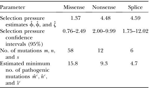
strong evidence of selection (P¼0.00029). In fact, the selection pressure estimates were similar for nonsense and splice mutations (c^ ¼4:48;^z¼4:59) but substan-tially lower for missense mutations (f^ ¼1:37), al-though the value for missense mutations is still greater than unity. The nonsense selection pressure was signif-icantly different from unity (P ¼ 0.0013). Similarly, TABLE 4

Significance levels comparing hypotheses H0, H1, H2, and H3

Mutation types H0vs. H1 H0vs. H2 H0vs. H3 H1vs. H2 H2vs. H3

All nonsynonymous point mutations 0.0943 0.00029 0.0046 0.00096 0.6368a

Missense mutations NA 0.2684 0.3905 NA 0.0829b

Nonsense mutations NA 0.0013 0.0105 NA 0.4164b

Splice site mutations NA 0.0068 0.0067 NA 0.0824b

Significances are split into missense, nonsense, splice, and combined effects. Exact tests were based upon 100,000 Monte Carlo simulations, unless otherwise indicated.

a_{An asymptotic likelihood-ratio test.}

b_{Based upon 10,000 simulations.}

TABLE 5

Parameter estimates

Parameter Missense Nonsense Splice

Selection pressure estimates ˆf;c, and ˆˆ z

1.37 4.48 4.59

Selection pressure confidence intervals (95%)

0.76–2.49 2.00–9.99 1.75–12.02

No. of mutationsm;n;

ands

58 12 6

Estimated minimum no. of pathogenic mutations ˆmc_;nˆc_;

and ˆsc

15.8 9.3 4.7

the splice site selection pressure was significant (P ¼

0.0068), but the missense selection pressure was not (P¼0.27). These observations suggest that the breast cancers exhibit stronger selection toward the protein-truncating mutations.

From Table 5, an estimated minimum of 29.8 of the 76 nonsynonymous mutations are pathogenic (39%), in-cluding 9.3 of the 12 nonsense mutations. In fact, 10 of the nonsense mutations arose from one sample, PD0119 (see Stephenset al. 2005 for details), suggest-ing that, at least for this tumor, cells accumulate growth advantage from multiple mutations, similar to the model of colorectal cancer evolution given by Little and Wright(2003).

The silent rate under the null hypothesis was esti-mated using Equation 6 to be 0.2460, suggesting that the silent:nonsilent ratio in the absence of selection will typically be1:3. Different mutation spectra or genome composition could substantially alter this, however.

Protein kinase domains are involved in the phosphor-ylation of proteins in signaling pathway cascades. These are highly conserved, implying that mutations within these regions are likely to affect protein function. Such mutations may enhance cell division and offer good can-didate oncogenic variants. Conversely, the cell may not tolerate mutations in such important regions, possibly inducing apoptosis, in which case protein-changing mutations will be avoided. Either scenario is indicative of selection pressures that vary according to the relative position of mutations with respect to the kinase do-mains. As such, all genes were split into three regions: prekinase, kinase, and postkinase, with each region hav-ing a separate selection parameter. Further details of the set of kinase genes can by found in the supplemen-tary information in Stephens et al. (2005). The exact positioning of these domains within the coding sequence can be found from a variety of database sources such as Ensembl (see Hubbardet al. 2005). Significant deviation of these parameters between the domains was then examined. The selection pressure for nonsense muta-tions varied significantly by position (P¼0.0053), with 9/12 mutations lying 39 to the kinase domain. This variation might suggest truncation of a regulatory

do-main or dodo-mains, while leaving the kinase dodo-main in-tact, free to drive the cancer.

In summary, these methods provide a straightforward and robust statistical approach to evaluating the impact of mutations identified in genomic screens on the devel-opment of cancer. Practical application to the kinase data has shown that the methods were able to demon-strate significant selection that varied among missense, nonsense, and splice variants. The use of such methods will be increasingly important in large-scale screens for somatic mutations in cancer.

We thank the Wellcome Trust and the Institute of Cancer Research for their support. D.F.E. is a Principal Research Fellow of Cancer Research United Kingdom.

LITERATURE CITED

Be´ roud_{, C., and T. S}oussi_{, 2003 The UMD-p53 database: new} mutations and analysis tools. Hum. Mutat.21:176–181. Cox_{, D. R., and D. V. H}inkley_{, 1974 Theoretical Statistics. Chapman &}

Hall, London.

Davies_{, H., G. R. B}ignell_{, C. C}ox_{, P. S}tephens_{, S. E}dkins_{et al.,} 2002 Mutations of the BRAF gene in human cancer. Nature

417:949–954.

Futreal, P. A., L. Coin, M. Marshall, T. Down, T. Hubbardet al., 2004 A census of human cancer genes. Nat. Rev. Cancer4:

177–183.

Goldman, N., and Z. Yang, 1994 A codon-based model of nucleo-tide substitution for protein-coding DNA sequences. Mol. Biol. Evol.11(5): 725–736.

Hall_{, B. G., 1990 Spontaneous point mutations that occur more} often when advantageous than when neutral. Genetics126:5–16. Hubbard_{, T., D. A}ndrews_{, M. C}accamo_{, G. C}ameron_{, Y. C}hen et al., 2005 Ensembl 2005. Nucleic Acids Res.33:D447–D453. Little_{, M. P., and E. G. W}right_{, 2003 A stochastic carcinogenesis} model incorporating genomic instability fitted to colon cancer data. Math. Biosci.183:111–134.

Sorensen_{, D., and D. G}ianola_{, 2002 Likelihood, Bayesian and MCMC} Methods in Quantitative Genetics. Springer, Berlin/Heidelberg, Germany/New York.

Stephens, P., S. Edkins, H. Davies, C. Greenman, C. Coxet al., 2005 A screen of the complete protein kinase gene family reveals diverse patterns of somatic mutations in human breast cancer. Nat. Genet.37:590–592.

Valverde, J. R., J. Alonso, I. Palaciousand A. Pestana, 2005 RB1 gene mutation up-date, a meta-analysis based on 932 reported mutations available in a searchable database. BMC Genet.6:53. Yang, Z., S. Roand B. Rannala, 2003 Likelihood models of somatic mutation and codon substitution in cancer genes. Genetics

165:695–705.