R E S E A R C H
Open Access
Finite-time control for uncertain systems
with nonlinear perturbations
Yuhong Liu
1*, Hui Li
1, Qishui Zhong
1and Shouming Zhong
2,3*Correspondence:
yhliu1210@163.com
1School of Aeronautics and
Astronautics, University of Electronic Science and Technology of China, Chengdu, 611731, China Full list of author information is available at the end of the article
Abstract
This study investigates the problem of finite-time control for uncertain systems with nonlinear perturbations. The aim is to design the state-feedback and output-feedback controller which ensure finite-time boundedness and with a desiredH∞performance index
υ
. Specifically, first, we divide the time-varying delay into non-uniformly subintervals and decompose the corresponding integral intervals to estimate the bounds of integral terms exactly. Second, the conditions obtained in this paper are formulated in terms of linear matrix inequalities (LMIs), which can be efficiently solved via standard numerical software. Finally, numerical examples are presented to demonstrate the effectiveness and advantages of the theoretical results.Keywords: finite-time boundedness (FTB); Lyapunov-Krasovskii functional (LKF); nonlinear perturbations
1 Introduction
Much work has been done on the robust control of linear systems over the past years [, ]. Most of the results in this field relate to the stability and performance criteria defined over an infinite time interval. In many practical applications, however, the main concern is the behavior of the system over a fixed finite time interval. In this sense it appears rea-sonable to define as stable a system whose state, given some initial conditions, remains within prescribed bounds in the fixed time interval, and as unstable a system which does not. Many are the practical problems in which this kind of stability (FTS) or short-time stability [, ] plays an important role: for instance the problem of not exceeding some given bounds for the state trajectories, when some saturation elements are present in the control loop; or the problem of controlling the trajectory of a space vehicle from an initial point to a final point in a prescribed time interval. Time delay frequently occurs in various practical engineering systems, such as static neural networks systems [, ], singular sys-tems [–], Markovian jump syssys-tems [–], genetic regulatory network syssys-tems [] and networked control systems (NCS) [–].
It is well known that the nonlinearities, as time delays also cause instability and poor per-formance of practical systems. Therefore, the stability problem of time-delay systems with nonlinear perturbations has received increased attention [–]. The free-weighting ma-trices approach was adopted in [–]. Recently, a less conservative delay-dependent sta-bility criterion was provided in [] by partitioning the delay interval into two segments of equal length, and evaluating the time derivative of a candidate LKF in each segment
of the delay interval into two segments of equal length, having this at our disposal, more information on the variation interval of the delay can be employed. Nevertheless, there still exists room for further improvement.
In many practical systems, time delay is unavoidable; see [–]. In such cases, a method of FTS has been applied to investigate the system with time varying; see [, ]. Motivated by the above discussions, this paper investigates the problem of finite-time con-trol for uncertain systems with nonlinear perturbations. The contributions of this paper can be summarized as follows:
• We divide the variation of the delay intoNparts with equal length, and construct a new LKF for these delay intervals, which can be regarded as an extension of the method of [], consequently, use more information of the delay range, and hence yield less conservative delay-range bounds.
• The system is assumed to be exactly known to designers in [],i.e., there are no uncertainties in the system, while in this paper, the existence of norm-bounded uncertainties is considered, which will increase the difficulty of FTS analysis.
• Only the state-feedback control is considered in [], in this paper, we design both the state-feedback and the output-feedback controllers, the output-feedback controller design is much more difficult than the state-feedback one.
• It is well known that a disturbance effect is often the source of instability and poor performance of a system, thus, the disturbance attenuation performance studied via theH∞control approach is worth to be considered. Compared with [, ], we added external disturbancew(t)and unknown nonlinear perturbationsf(x(t),t),
g(x(t–τ(t)),t), and this motivates the research.
In this paper, we deal with the problem of finite-timeH∞controller design for uncer-tain systems with nonlinear perturbations. Both state-feedback controller and output-feedback controller have been considered. By means of LMI techniques, some suffi-cient LMI-based conditions for the existence of the state-feedback controller and output-feedback controller are given.
The rest of the current paper is organized as follows. Section introduces the problem formulation and some definitions on FTB and finite-timeH∞control. Some FTB criteria obtained for the systems are presented in Section . In Section , the problem of finite-timeH∞control via state-feedback and output-feedback is discussed. Section gives some
numerical examples to demonstrate the effectiveness of our main results. Finally, Section draws the conclusion.
Notation The superscriptsT and (–) stand for matrix transposition and matrix in-verse, respectively;Rn denotes then-dimensional Euclidean space; the notationX>Y
(X≥Y), whereX,Yare symmetric matrices, means thatX–Yis positive definite (posi-tive semidefinite).∗denotes the term that is induced by symmetry.col{x,x, . . . ,xn}means
[xT
,xT, . . . ,xTn]TandSym{X}=X+XT. The shorthand notationdiag{M,M, . . . ,Mn}
de-notes a block diagonal matrix with diagonal blocks being the matrices M,M, . . . ,Mn.
λmin(·) andλmax(·) denote the smallest and largest eigenvalue of·. Ln[N] is the space
2 Problem formulation and preliminaries
In this paper, we consider the neural networks with time-varying delay systems as follows:
⎧ ⎪ ⎪ ⎪ ⎪ ⎪ ⎨ ⎪ ⎪ ⎪ ⎪ ⎪ ⎩ ˙
x(t) = [A+A(t)]x(t) + [Ad+Ad(t)]x(t–τ(t)) +Ff(x(t),t)
+Gg(x(t–τ(t)),t) +Bu(t) +Ew(t),
y(t) =Cx(t) +Cdx(t–τ(t)),
x(t) =ϕ(t), t∈[–τM, ],
()
wherex(t)∈Rnis the state vector of the neural network associated with n neurons;τ(t)
is time-varying delay satisfying <τm≤τ(t)≤τM,τ˜d≤ ˙τ(t)≤ ¯τd;ϕ(·)∈L[–τM ] is
an initial function;u(t)∈Rl is the control input andy(t)∈Rm is the measured output.
w(t)∈Lq[ +∞] is the external disturbances;A, Ad, C, Cd,F, G,B, E are known real
constant matrices with appropriate dimensions.A(t),Ad(t) are real-valued unknown
matrices representing time-varying parameter uncertainties, and they are assumed to be of the form
A(t) Ad(t)
=L(t)Ea Ed
, ()
where LandEi(i=a,d) are known real constant matrices and(t) is unknown
time-varying matrix functions satisfyingT(t)(t)≤I,∀t.f(x(t),t)∈Rnandg(x(t–τ(t)),t)∈ Rnare unknown nonlinear perturbations withx(t) andx(t–τ(t)), respectively. They satisfy
f(,t)≡,g(,t)≡, and
⎧ ⎨ ⎩
fT(x(t),t)f(x(t),t)≤αxT(t)x(t),
gT(x(t–τ(t)),t)g(x(t–τ(t)),t)≤βxT(t–τ(t))x(t–τ(t)), ()
whereα≥,β≥ are known scalars. For simplicity we denotef =f(x(t),t),g=g(x(t– τ(t),t)).
Assumption . For any given positive numberη, the external disturbances inputw(t) is
time varying and satisfies
T
wT(t)w(t)dt≤η, η≥. ()
In this paper, the objective is to find a state-feedback controller and output-feedback controller for the system () that will render the corresponding closed-loop dynamic sys-tem FTB with a desiredH∞ indexυ. The definitions of FTS, FTB and finite-timeH∞
control are introduced as follows.
Definition .([] (FTS)) The time-delay system () withw(t) = is said to be FTS with
respect to (c,c,T,R), wherec> , andR> , if there exists a constantc(>c), such that
Definition . ([] (FTB)) Given positive constants c, η, T and a symmetric
ma-trix R> , the time-delay system () with w(t) satisfying () guaranteed by the state-feedback/output-feedback controller is said to be robustly FTB with respect to (c,c,T,
R,η), if there exists a constantc(>c), such that
xT(t)Rx(t)≤c, ∀t∈(–τM, ] ⇒ xT(t)Rx(t)≤c, ∀t∈(,T],
Definition .([]) If there exists a state-feedback/an output-feedback controller, such that the closed-loop system is FTB with respect to (c,c,T,R,η) and under the assumed
zero initial condition, the system output satisfies the following cost function inequality for
T> and for all admissiblew(t) which satisfy ():
T
yT(t)y(t)dt≤υ
T
wT(t)w(t)dt. ()
Then the state-feedback/out-putback controller is called the robust finite-timeH∞
con-troller of the system ().
Remark (FTS and asymptotic stability) It is worth noting that asymptotic stability and FTS are independent concepts: a system which is FTS may not be asymptotically stable, while an asymptotically stable system may not be FTS.
Remark It is easy to see that, given Definition . of FTB, FTS can be recovered as a particular case by lettingη= .
Remark From system (), combining (), (), (), it follows that
ϕ(˙ t) ≤A+Ad+LEa+Ed+αF+βGϕ+Eη
=√ρ, ∀t∈[–τM, ]. ()
We note that
ρ=A+Ad+LEa+Ed+αF+βGϕ+Eη.
Lemma .([]) For any positive matrix Z and for differentiable signal x in[α,β]→Rn,
the following inequality holds:
β
α
˙
xT(u)Zx˙(u)≥ β–αˆ
TZ¯,ˆ
whereZ¯=diag{Z, Z}and
ˆ
=
x(β) –x(α)
x(β) +x(α) –β–ααβx(u)du
.
Lemma .([]) Let H,E,and F(t)be real matrices of appropriate dimension with F(t)
satisfying
FT(t)F(t)≤I.
Then for any scalarε>
HF(t)E+HF(t)ET≤ε–HHT+εETE.
3 Main results
In this section, we shall establish our main results based on LMI framework. LetN> be an integer andτj(j= , , . . . ,N+ ) be some scalars satisfying
τm=τ<τ<· · ·<τN<τN+=τM.
We can divide the delay interval [τm,τM] intoNequidistant subintervals, whereτm=τ,
τN+=τM, we denote byτthe length of the subinterval [τi,τi+], that is,τ=τi+–τi=
(τM–τm)
N . Firstly, we derive sufficient conditions which guarantee the FTB of system in
equa-tion () under ignoring the control inputu(t), secondly, we will consider an unstable sys-tem, respectively, design the state-feedback and output-feedback controller to make the system FTB.
3.1 A new model transformation
To extract the time-varying term inτ(t), we expressx(t–τ(t)) as
xt–τ(t)=δx(t–τi) + ( –δ)x(t–τi+) +δτχd(t), ()
whereδ∈(, ],δx(t–τi)+(–δ)x(t–τi+) denotes the approximation ofx(t–τ(t)),δτχd(t)
is the approximation error. Ignoring the control inputu(t), by using equation (), the sys-tem in () can be regarded as
˙
x(t) =Ax¯ (t) +δA¯dx(t–τi) + ( –δ)A¯dx(t–τi+) +δτA¯dχd(t) +Ff+Gg+Ew(t), ()
where
¯
Remark In [],x(t–τ(t)) is expressed byx(t–τ(t)) =x(t–τ) +(t–τ) +τχd(t).
In this paper, we useδ (δ∈(, ]) instead of . In this way, we can get less conservative criteria for delay systems via adjusting the parameterδ.
By definingyd(t) =x˙(t), we can rewriteχd(t) as
χd(t) =
δτ
xt–τ(t)–δx(t–τi) – ( –δ)x(t–τi+)
=
δτ
( –δ)xt–τ(t)–x(t–τi+)
–δx(t–τi) –x
t–τ(t)
= –δ
δτ
t–τ(t)
t–τi+
˙
x(s)ds– τ
t–τi
t–τ(t)
˙
x(s)ds
=
τ
t–τi
t–τi+
σ(θ)yd(θ)dθ, ()
where
σ(θ) =
⎧ ⎨ ⎩
–δ
δ , t–τi+≤θ<t–τ(t),
–, t–τ(t)≤θ≤t–τi.
Hence, equation () can be written as
yd(t)
y(t)
=
ζ(t)
χd(t)
, ()
where
ζ(t) =col
x(t),x(t–τi),x(t–τi+),f,g,
t
t–τi
x(s)ds,
t–τi
t–τi+
x(s)ds,w(t)
,
T =colA¯T,δA¯Td, ( –δ)A¯Td,FT,GT, , ,ET,δτA¯Td
,
T =colCT,δCdT, ( –δ)CdT, , , , , ,δτCdT.
For convenience of representation, the following notation is introduced:
ei=col{ n, . . . , n
i–
,In, n, . . . , n
–i },
ξT(t) =ζT(t) χdT(t).
In order to derive less conservative criteria, we firstly analyze the method of choosing LKF for the above-mentioned systems () and asymptotically stable conditions are pre-sented in this section.
3.2 FTB analysis
=PG, =P+P+PT+P+ATP+ATP+
The other entries ofare zeros.We have
Calculating the time derivative ofV(xt) along the solution of (), we can get
Using Lemma ., one obtains
where
it asM, using Jensen’s inequality []
–τ
Combining equations ()-(), we obtain
whereˆ = (ˆij)×.
ˆ
=PA¯+A¯TP+P+PT+P+PT+Q+Q+εαI+A¯TSA¯– – ,
ˆ
=δPA¯d–P+δA¯TSA¯d– ,
ˆ
= ( –δ)PA¯d–P+ ( –δ)A¯TSA¯d– , ˆ=PF+A¯TSF,
ˆ
=PG+A¯TSG,
ˆ
=P+P+PT+P+A¯TP+A¯TP+
τi
+
τi+
,
ˆ
=A¯TP+P+P+
τi+
, ˆ=A¯TSE+PE,
ˆ
=δτPA¯d+δτA¯TSA¯d, ˆ= –Q+δA¯TdSA¯d+εβδI– ,
ˆ
=δ( –δ)A¯TdSA¯d+εβδ( –δ)I, ˆ=δA¯TdSF, ˆ=δA¯TdSG, ˆ
= –P–P+δA¯Td(P+P) +
τi
, ˆ= –P+δA¯TdP,
ˆ
=δA¯TdSE, ˆ=δτA¯TdSA¯d+εβδτI,
ˆ
= –Q– +βε( –δ)I+ ( –δ)A¯TdSA¯d, ˆ= ( –δ)A¯TdSF, ˆ
= ( –δ)A¯TdSG, ˆ=
τi+
+ ( –δ)A¯Td(P+P) –PT–P,
ˆ
=
τi+
+ ( –δ)A¯TdP–P, ˆ= ( –δ)A¯TdSE, ˆ
=εβ( –δ)δτI+ ( –δ)δτA¯dTSA¯d, ˆ= –εI+FTSF,
ˆ
=FTSG, ˆ=FT(P+P), ˆ=FTP,
ˆ
=FTSE, ˆ=δτFTSA¯d, ˆ= –εI+GTSG,
ˆ
=GT(P+P), ˆ=GTP, ˆ=GTSE, ˆ=δτGTSA¯d, ˆ
= –
τ
i
–
τ
i+
, ˆ= –
τ
i+
, ˆ=
PT +PTE,
ˆ
=δτ
PT+PTA¯d, ˆ= –
τi+, ˆ=P
T
E,
ˆ
=δτPTA¯d, ˆ=ETSE, ˆ=δτETSA¯d, ˆ
= –τM+εβδτI+δτA¯TdSA¯d.
Next, choosing a supplementary function asJ(t) =V˙i(xt) –γxT(t)Px(t) –γwT(t)w(t),
it follows that
J(t)≤ξT(t)ξ˜ (t), ()
where˜ = (˜ij)×,
˜
=PA¯+A¯TP+P+PT + +P+PT +Q+Q+εαI
˜
By using the Schur complement [], it is obvious that the inequality in equation () is equivalent to
Using equation (), the inequality in equation () can be rewritten as
Applying Lemma ., the inequality in equation () is equivalent to equation (). Hence, if the condition in equation () holds, we haveJ(t)≤ξT(t)ξ˜ (t) < . Then we can obtain
˙
Vi(xt) <γxT(t)Px(t) +γwT(t)w(t) <γVi(xt) +γwT(t)w(t). ()
Multiplying the above inequality bye–γt, it yields
d
By integrating the aforementioned inequality between andt, we obtain
V(xt) <eγtV(x) +γeγt
The initial value of LKF can be written as
In addition, combining equations ()-(), we have
λmin(P˜)xT(t)ψx(t)≤eγT
xT()Px() +
+eγTη –e–γT, t∈(,T], () it follows from () that
xT(t)ψx(t)≤cλmax(P˜) ++η( –e
–γT)
λmin(P˜)e–γT
. ()
Now, we proceed to show the derivation of conditions of () and (). In order to trans-form () into a LMI-based condition, we assume that inequality () is true, that is,
ψ<P
P< ψ
(
⇒ I<ψ–/Pψ–/< I.
The above relations imply thatλ> ,λ< . By considering these relations, one can obtain
the following:
⎧ ⎨ ⎩
cλ+ω+η( –e–γT) < c+ω+η( –e–γT),
cλe–γT>ce–γT.
Definingλ=λmin(P˜),λ=λmax(P˜), we arrive atxT(t)ψx(t) <cfrom LMIs () and ().
That is, the system in () is FTB when ignoring the control inputu(t). This completes the
proof.
Remark Different from the partitioning approach used in [], when the delay-partitioning number becomes larger, there are involved more decision variables, so that the conditions become more complicated and the computational cost increases. However, in our method, there are no additional matrix variables apart from those associated in the corresponding LKF, that is,P,Qi(i= , ),Xj(j= , , , , ). One can see that when the
delay-partitioning number becomes larger, the derived criteria can lead to an improve-ment. Furthermore, the cost of computation and the complexity of the obtained criteria do not increase.
Remark If there is no perturbation, that is,f = ,g= ,w(t) = , the FTB problem of system () is reduced to analyzing the FTS of the system
⎧ ⎪ ⎪ ⎨ ⎪ ⎪ ⎩ ˙
x(t) = [A+A(t)]x(t) + [Ad+Ad(t)]x(t–τ(t)) +Bu(t),
y(t) =Cx(t) +Cdx(t–τ(t)),
x(t) =ϕ(t), t∈[–τM, ].
This problem has been widely studied in the recent literature (see []) and the FTS crite-rion for the deterministic system is addressed below.
Remark The inequalities in equations ()-() are LMIs, which can be calculated by the LMI toolbox in MATLAB. The results depend on the selected parameters (c,c,T,ψ,η),
the lower and upper bounds of the time-varying delay, and scalars εandγ. Further, in order to obtain a minimum state upper boundc, we choose a value of the parameterε,
then the minimum searching function (such as the “mincx” in MATLAB) can be used to search an optimalγ which can guarantee the upper boundcminimum.
3.3 State-feedback controller design
In this subsection, we consider the following state-feedback controller for the system ():
u(t) =Kx(t), ()
where the state-feedback controller gainKis to be determined in the course of the design. Then we can get the following closed-loop system:
⎧
Theorem . gives sufficient conditions, which guarantee the resulting closed-loop system () is FTB with respect to the given (c,c,T,ψ,η).
Theorem . For some given scalarsα,β,c,η, <τm≤τM,τ˜d,ψ,τ¯d,δ∈(, ],T > ,
γ ≥,ρ,the system in()by the state-feedback controller()is FTB with respect to
(c,c,T,ψ,η)and satisfies the cost function equation()for all admissible w(t),if there
exist symmetric positive matrices P=
The other entries of are the same asin Theorem..We have
=
τi(XA+W) τiδXAd τi( –δ)XAd τiXF τiXG τiXE ττiδXAd
T
,
=
τi+(XA+W) τi+δXAd τi+( –δ)XAd τi+XF τi+XG
τi+XE ττi+δXAd
T
,
=
τ(XA+W) τδXAd τ( –δ)XAd τXF τXG τXE τδXAd
T
,
=
τ(XA+W) τδXAd τ( –δ)XAd τXF τXG τXE τδXAd
T
,
=
τ(XA+W) τδXAd τ( –δ)XAd τXF τXG τXE τδXAd
T
,
=
εLTP ε(κ+κ)LTP εκLTP
T
,
∗=τiω+τi+ω+ τiκω+ τi+κω+ τiτi+ω+τiω+τi+ω
c
λmin(ψ)
+
τi ω+
τi+ ω+
τ
(τi+τi+)ω+τω – τi
+
τi+
!
+τω –
τi
+
τi+
!
ρ.
In this case,a suitable state-feedback controller gain can be obtained by K= (BTB)–×
BTP–W.
Proof Select the same KLF as Theorem . and define the following function:
J(t) =V˙i(xt) –γxT(t)Px(t) –γwT(t)w(t) +
σy
T(t)y(t).
Recalling the condition equation (), we have the following relation along the trajecto-ries of system:
J(t) < .
Then we obtain the following equation through some similar algebraic manipulations of the proof in Theorem .:
T
yT(t)y(t)dt<σ γeγT
T
wT(t)w(t)dt.
Therefore, condition () can be guaranteed by lettingv=σ γeγT. By means of the change
of variableW=PBK,W=XBK,W=XBK,W=XBK,W=XBK,W=XBK, the
proof procedure is similar to that of Theorem ., and it is omitted here.
3.4 Output-feedback controller design
In this subsection, we consider the following output-feedback controller for the system ():
where the state-feedback controller gainKis to be determined in the course of the design. Then we can get the following closed-loop system:
⎧
Theorem . presents some sufficient conditions which guarantee the resulting closed-loop system () is FTB with respect to the given (c,c,T,ψ,η).
Theorem . For some given scalarsα,β,c,η, <τm≤τM,τ˜d,ψ,τ¯d,δ∈(, ],T > ,
γ ≥,ρ,the system in()by the output-feedback controller()is FTB with respect to
(c,c,T,ψ,η)and satisfies the cost function equation()for all admissible w(t),if there
exist symmetric positive matrices
Proof The closed-loop system in equation () can be written as
˙
The proof procedure is similar to that of Theorem ., and it is not difficult to get the
conclusion. This completes the proof.
4 Numerical examples and simulation
Example Consider the system () with the parameters []
Figure 1 State responsex(t) of the system with state-feedback controller and time-varying delay 0.1≤τ(t)≤2.2.
Figure 2 Time-delay state responsex(t–τ(t)) of the system with state-feedback controller and time-varying delay 0.1≤τ(t)≤2.2.
using Theorem ., the control gain matrix K and the minimum upper bound of state variable are calculated by LMIs in equations (), (), (), (), () forγ= .. When i=,τ(t)∈[., .]
min{c}= .e+ ,
P=
. .
. .
, W= .e+ ∗
–. .
–. –.
,
K= .e+ ∗[–. –.].
•Output-feedback case: We chooseα= ,β= ,η= .,ρ= .,T= .,c= .,
ε= ,,ψ=I,k= .,k= .,τ˜d= .,τ¯d= .,τm= .,τM = .,N= . By
using Theorem ., the control gain matrix K and the minimum upper bound of state variable are calculated by LMIs in equations (), (), (), (), (), forγ = .. When
i= ,τ(t)∈[., .],
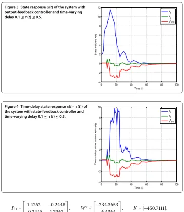
Figure 3 State responsex(t) of the system with output-feedback controller and time-varying delay 0.1≤τ(t)≤0.5.
Figure 4 Time-delay state responsex(t–τ(t)) of the system with state-feedback controller and time-varying delay 0.1≤τ(t)≤0.5.
P=
. –.
–. .
, Wo=
–. –.
, K= [–.].
The curves of state values with state-feedback controller and output-feedback controller are shown in Figures -.
From Figures -, it can be seen that state values satisfy the following condition with the state-feedback controller:K= .e+ ∗[–. –.], which makes the unstable system in () FTB with respect to (., ,, .,I, .). We have
xT(t)ψx(t) <c= ,, ∀t∈(, .].
Further, with the output-feedback controllerK= [–.], state responses satisfy the following condition, which proves that the system is FTB with respect to (., ,, .,
I, .):
xT(t)ψx(t) <c= ,, ∀t∈(, .].
Whenτm= .,k= .,k= .,α=β= , the minimum allowable upper bounds for
Figure 5 The system with state-feedback controller wheni= 2.
Figure 6 The system with state-feedback controller wheni= 3.
Table 1 The minimum allowablec2upper bound forτmwith different valuesi
i 1 2 3 4 5 6
State-Feedback Case 8.3992e+04 2.143e+05 3.3919e+05 1.8940e+07 9.0078e+07 3.0874e+08 Output-Feedback Case 1.4127e+04 7.3132e+03 9.1025e+05 5.7247e+06 1.1926e+07 9.8105e+06
criteria can still be applicable when the range ofcis greater by adjusting the parameteri.
From Figures -, we can see that with output-feedback controller, the state values are larger and the rate of convergence is faster than those with state-feedback controller.
Example We consider the above time-delay systems () with the following parameters given in [, , , ]:
A=
–. .
–. –
, Ad=
–. .
– –.
, B=
, C= [ ],
Cd= [ ], L=
Figure 7 The system with output-feedback controller wheni= 2.
Figure 8 The system with output-feedback controller wheni= 3.
F=G=
, E=
.
For given values ofα= .,β= .,c= .,ρ= .,η= .,τ˜d= .,τ¯d= .,
ε= ,δ= .,T= .,τm= ,τM= .,ψ=I,N= , we provide a part of the feasible
solution here (due to the limitation of the length of this paper):
c{min}= .e+ ,
Q=
. .
. .
, Q=
. –.
–. .
,
ε= ., ε= ..
Letf(x) = .x(t)sin(x(t)),g(x(t–τ(t))) = .x(t–τ(t))cos(x(t–τ(t))), in this exam-ple, Figures and show the trajectory of variablesx(t) with τM = . andτ(t) =
+ .sintunder the initial condition [., .], respectively.
Whenα=β= .,τm= ,τM= .,τ˜d= .,τ¯d= ., the minimum allowablec are
Figure 9 Trajectories ofx(t) withτ= 8.3618.
Figure 10 Trajectories ofx(t) withτ(t) = 8 + 0.25 sin(t).
Table 2 The minimum allowablec2upper bound forτmwith different valuesδ
δ 0.5 0.6 0.7 0.9
min{c2} 4.1132e+06 1.4459e+07 3.6054e+07 8.8196e+06
Example We consider the above time-delay systems () with the following parameters
given in []:
A=
– .
–
, Ad=
–
– –
, B=
, C= [ ],
Cd= [ ], L=
, Ea= [ ], Ed= [ ],
F=G=
, E=
.
Letf(x(t)) = .x(t)∗sin(x(t)),g(x(t–τ(t))) = .x(t–τ(t))∗cos(x(t–τ(t))),τM= ..
Figure 11 Trajectories ofx(t) withτ= 8.5419.
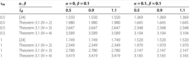
Table 3 Maximum boundsτMforτm= 0.5, 1
τm α,β α= 0,β= 0.1 α= 0.1,β= 0.1
¯
τd 0.5 0.9 1.1 0.5 0.9 1.1
0.5 [24] 1.550 1.550 1.550 1.369 1.369 1.369
0.5 Theorem 3.1 (N= 2) 1.980 1.980 1.980 1.645 1.645 1.645
0.5 Theorem 3.1 (N= 3) 2.647 2.647 2.647 2.348 2.348 2.348
0.5 Theorem 3.1 (N= 4) 3.589 3.589 3.589 3.104 3.104 3.104
1 [24] 1.749 1.749 1.749 1.520 1.520 1.520
1 Theorem 3.1 (N= 2) 2.349 2.349 2.349 1.970 1.970 1.970
1 Theorem 3.1 (N= 3) 2.780 2.780 2.780 2.147 2.147 2.147
1 Theorem 3.1 (N= 4) 3.419 3.419 3.419 3.165 3.165 3.165
For given values ofα,βandτ¯d, we apply Theorem . to calculate the maximal allowable
valueτM that guarantees the asymptotical stability of the system listed in Table . From
the table, it is easy to see that our proposed stability criterion gives much less conservative results than those in [], since the proposed analysis uses delay-partitioning approach as well as tighter bounding on the time derivative of the LKF.
5 Conclusions
In this paper, we investigated the finite-timeH∞control problem for a class of
continuous-time nonlinear system with continuous-time-varying norm-bounded parameter uncertainties and ad-missible external disturbances. Some sufficient conditions for the existence of the robust state-feedback controller and output-feedback controller have been provided in terms of LMIs. Finally, numerical examples are provided to demonstrate the effectiveness of the proposed method.
Competing interests
The authors declare that there is no conflict of interest regarding the publication of this paper.
Authors’ contributions
YHL carried out the main part of this article, HL and SMZ corrected and revised the manuscript, QSZ brought forward some suggestions on this article. All authors have read and approved the final manuscript.
Author details
1School of Aeronautics and Astronautics, University of Electronic Science and Technology of China, Chengdu, 611731,
China.2School of Mathematical Sciences, University of Electronic Science and Technology of China, Chengdu, 611731,
China.3Key Laboratory for Neuroinformation of Ministry of Education, University of Electronic Science and Technology of
Acknowledgements
The authors greatly appreciate the reviewers suggestions and the editors’ encouragement. The work is partially supported by the National Basic Research Program of China (2010CB732501) and the Sichuan Science and Technology Plan (2014GZ0079).
Received: 19 July 2016 Accepted: 14 January 2017
References
1. Bhattacharyya, S, Chapellat, H, Keel, L: Robust Control: The Parametric Approach. Pearson Education, Upper Saddle River (1995)
2. Zhou, K, Doyle, JC: Essentials of Robust Control. Prentice Hall, Upper Saddle River (1998) 3. Dorato, P: Short-time stability in linear time-varying systems. DTIC Document (1961)
4. Weiss, L, Infante, E: Finite time stability under perturbing forces and on product spaces. IEEE Trans. Autom. Control12, 54-59 (1967)
5. Zeng, HB, Park, JH, Zhang, CF, Wang, W: Stability and dissipativity analysis of static neural networks with interval time-varying delay. J. Franklin Inst.352, 1284-1295 (2015)
6. Wu, ZG, Lam, J, Su, H, Chu, J: Stability and dissipativity analysis of static neural networks with time delay. IEEE Trans. Neural Netw. Learn. Syst.23, 199-210 (2012)
7. Zhang, Y, Liu, C, Mu, X: Robust finite-time stabilization of uncertain singular Markovian jump systems. Appl. Math. Model.36, 5109-5121 (2012)
8. Rakkiyappan, R, Kaviarasan, B, Rihan, FA, Lakshmanan, S: Synchronization of singular Markovian jumping complex networks with additive time-varying delays via pinning control. J. Franklin Inst.352, 3178-3195 (2015)
9. Wu, ZG, Park, JH: MixedH∞and passive filtering for singular systems with time delays. Signal Process.93, 1705-1711 (2013)
10. Wu, ZG, Park, JH: Reliable passive control for singular systems with time-varying delays. J. Process Control23, 1217-1228 (2013)
11. Yao, DY, Lu, Q: Robust finite-time state estimation of uncertain neural networks with Markovian jump parameters. Neurocomputing159, 257-262 (2015)
12. Xing, X, Yao, DY: Finite-time stability of Markovian jump neural networks with partly unknown transition probabilityes. Neurocomputing159, 282-287 (2015)
13. Wang, GL, Bo, HY:H∞Filtering for time-delayed singular Markovian jump systems with time-varying switching: a quantized method. Signal Process.109, 14-24 (2015)
14. Wang, JR, Wang, HJ: Delaye-dependentH∞control for singular Markovian jumping systems with time delay. Nonlinear Anal. Hybrid Syst.8, 1-12 (2013)
15. Wu, ZG, Park, JH, Su, H, Chu, J: Delay-dependent passivity for singular Markov jump systems with time-delays. Commun. Nonlinear Sci. Numer. Simul.18, 669-681 (2013)
16. Lakshmanan, S, Rihan, FA, Rakkiyappan, R, Park, JH: Stability analysis of the differential genetic regulatory networks model with time-varying delays and Markovian jumping parameters. Nonlinear Anal. Hybrid Syst.14, 1-15 (2014) 17. Zhang, Z, Zhang, Z, Zhang, H: Finite-time stability analysis and stabilization for uncertain continuous-time system
with time-varying delay. J. Franklin Inst.352, 1296-1317 (2015)
18. Song, J, He, S: Robust finite-timeH∞control for one-sided Lipschitz nonlinear systems via state feedback and output feedback. J. Franklin Inst.352, 3250-3266 (2015)
19. Ali, MS, Saravanakumar, R: Novel delay-dependent robustH∞control of uncertain systems with distributed time-varying delays. Appl. Math. Comput.249, 510-520 (2014)
20. Amato, F, Ariola, M: Finite-time control of linear systems subject to parametric uncertainties and disturbances. Automatica37, 1459-1463 (2001)
21. Song, J, He, SP: Finite-time robust passive control for a class of uncertain Lipschitz nonlinear systems with time-delays. Neurocomputing159, 275-281 (2015)
22. Wang, WQ, Nguang, SK: Novel delay-dependent stability criterion for time-varying delay systems with parameter uncertainties and nonlinear perturbations. Inf. Sci.281, 321-333 (2014)
23. Kwon, OM, Park, MJ: Improve results on stability of linear systems with time-varying delays via Wirtinger-based integral inequality. J. Franklin Inst.351, 5586-9398 (2014)
24. Hui, JJ, Kong, XY, Zhang, HX, Zhou, X: Delay-partitioning approach for systems with interval time-varying delay and nonlinear perturbations. J. Comput. Appl. Math.281, 74-81 (2015)
25. Qian, W, Li, T: Stability analysis for interval time-varying delay systems based on time-varying bound integral method. J. Franklin Inst.351, 4892-4903 (2014)
26. Seuret, A, Gouaisbout, F: Wirtinger-based integral inequality: application to time-delay systems. Automatica49, 2860-2866 (2013)
27. Balasurbramaniam, P, Nagamani, G: A delay decomposition approach to delay-dependent passivity analysis for interval neural networks with time-varying delay. Neurocomputing74(10), 1646-1653 (2011)
28. Zhang, Z, Zhang, Z, Zhang, H, Zheng, B, Karimi, HR: Finite-time stability analysis and stabilization for linear discrete-time system with time-varying delay. J. Franklin Inst.351(6), 3457-3476 (2014)
29. Ramakrishnan, K, Ray, G: Delay-range-dependent stability criterion for interval time-delay systems with nonlinear perturbations. Int. J. Autom. Comput.8, 141-146 (2011)
30. Zhang, W, Cai, XS, Han, ZZ: Robust stability criteria for systems with interval time-varying delay and nonlinear perturbations. J. Comput. Appl. Math.234, 174-180 (2010)
31. Lu, JQ, Ho, DWC, Cao, JD: Synchronization in an array of nonlinearly coupled chaotic neural networks with delay coupling. Int. J. Bifurc. Chaos18(10), 3101-3111 (2008)
32. Lu, JQ, Wang, ZD, Cao, JD, Ho, DWC, Kurths, J: Pinning impulsive stabilization of nonlinear dynamical networks with time-varying delay. Int. J. Bifurc. Chaos22(7), 1250176 (2012)
34. Zhang, BY, Xu, SY, Lam, J: Relaxed passivity conditions for neural networks with time-varying delays. Neurocomputing
142, 299-306 (2014)
35. Grantham, WJ: Estimating controllability boundaries for uncertain systems. In: Renewable Resource Management, pp. 151-162. Springer, Berlin (1981)