R E S E A R C H
Open Access
Hopf-zero bifurcation of Oregonator
oscillator with delay
Yuting Cai
1, Liqin Liu
1*and Chunrui Zhang
1*Correspondence:
fymm007@163.com
1Department of Mathematics,
Northeast Forestry University, Heilongjiang, China
Abstract
In this paper, we study the Hopf-zero bifurcation of Oregonator oscillator with delay. The interaction coefficient and time delay are taken as two bifurcation parameters. Firstly, we get the normal form by performing a center manifold reduction and using the normal form theory developed by Faria and Magalhães. Secondly, we obtain a critical value to predict the bifurcation diagrams and phase portraits. Under some conditions, saddle-node bifurcation and pitchfork bifurcation occur alongMandN, respectively; Hopf bifurcation and heteroclinic bifurcation occur alongHandS, respectively. Finally, we use numerical simulations to support theoretical analysis.
MSC: 34K18; 35B32
Keywords: Oregonator model; Delay; Hopf-zero bifurcation; Normal form
1 Introduction
An oscillatory chemical reaction refers to the reaction system of certain antileather con-centration showing relatively stable cyclical changes. In 1921, Bray achieved a liquid oscil-latory reaction in the experiment. In 1964, Zhabotinsky reported some other osciloscil-latory reactions of this nature [14,15,21]. Until the 1970s, Field, Koros, and Noyes proposed the Oregonator model based on an in-depth study of the BZ reaction. According to Field and Noyes, theBZreaction is simplified. In 1979, Tyson assumed that the concentration of the reactantsA= [BrO–3] andB= [BrCH(COOH)2] is independent of time. Therefore we can give the following reactant concentration equation:
⎧ ⎪ ⎪ ⎨ ⎪ ⎪ ⎩
dP
dt =k3AQ–k2PQ+k5AP– 2k4P2, dQ
dt =k3AQ–k2PQ+
1 2fk0BW,
dW
dt = 2k5AP–k0BW,
whereP= [HBrO2],Q= [Br],W= [Ce(IV)]. We will make the following changes in this system:
x=αP, y=βQ, z=γW, t=δT, where
α≈ 2k4
k3A≈
106(mol/L)–1, β= k2
k3A≈
2×10⁷(mol/L)–1,
γ ≈ k4k5B
(k3A)3
≈20 (mol/L)–1, δ=k5B≈4×10⁻³s–1.
So we can obtain another form of the Oregonator oscillator, the so-called Tyson-type os-cillator:
⎧ ⎪ ⎪ ⎨ ⎪ ⎪ ⎩
εdxdt =qy–xy+x(1 –x),
δdydt= –qy–xy+h1z,
dz dt =x–z,
where
ε=k5B
k3A≈
4×10⁻², δ=εα
β ≈2×10
–6, q=2k1k4 k2k3 ≈
10–5, h1= 2h1.
Becauseδis much smaller thanε, the second formula in the system can be approximated as
y≈ h1z q+x.
This yields a simplified two-dimensional Oregonator model [27] with respect toxandz:
⎧ ⎨ ⎩
εdxdt =x(1 –x) –h1zxx–+qq,
dz dt =x–z,
(1.1)
wherex= [HBrO2],z= Ce(IV).
When electric current is applied, the catalyst Ce(IV) is perturbed, and other species are not affected (see [15]). Since the perturbation term is introduced in the equationdzdt =x–z, we rewrite this equation in the following form:
dz
dt=x–z+kz(t–τ).
We consider the Oregonator model with delay:
⎧ ⎨ ⎩
εdxdt =x(1 –x) –h1zxx–+qq,
dz
dt =x–z+kz(t–τ),
(1.2)
whereε= 4×10⁻²,δ= 4×10⁻⁴,q= 8×10⁻⁴, andh
1∈(0, 1) is an adjustable parameter. Nowadays, many scholars study the Hopf bifurcation or Hopf-zero bifurcation in delay differential equations, and some results have been obtained (see [1,2,4,5,7–10,12,13,
17,19,22,24,26–29]). However, to the best of our knowledge, there are no studies on the Hopf-zero bifurcation of Oregonator oscillator with time delay. Therefore, it is the far-reaching significance to research the Hopf-zero bifurcation of Oregonator model.
form method [6,23] to investigate the Hopf-zero bifurcation with original parameters. In Sect.4, we give several numerical simulations to support the analytic results. Finally, we draw the conclusion in Sect.5.
2 Stability and existence of Hopf-zero bifurcation
Let (x,z) be an equilibrium point of system (1.2). Obviously,
⎧ ⎨ ⎩
x(1 –x) –h1zxx–+qq= 0,
z=1–xk.
Then we have
x(1 –x) – h1 1 –kx
x–q
x+q= 0. (2.1)
There are three rootsx= 0,x=x+, andx=x–of Eq. (2.1), where
x±=
1 –1–h1k–q±
(1 –1–h1k–q)2+ 4q(1 + h1 1–k)
2 . (2.2)
Therefore we obtain that system (1.2) has three steady-state solutions, (x–,z–), (0, 0), and (x+,z+).
Obviously, there is a unique positive steady state.
Theorem 2.1 For anyε> 0,q> 0,and h1> 0, (x+,z+)is the unique positive steady state of system(1.2).
Proof LetH(x) =x(1 –x) –1–h1kxxx–+qq. From (2.1) and (2.2) we get that onlyx+satisfiesH(x) = 0,H(x) > 0 for 0 <x<x+, andH(x) < 0 forx>x+. Furthermore, we haveH(x+) = 0 and
H(x+) < 0.
We further mainly study the dynamics of the equilibrium point (x+,z+). If the characteristic equation of system (1.2) has a simple pair of purely imaginary eigenvalues±iω, a simple root 0, and all other roots of the characteristic equation have negative real parts, then the Hopf-zero bifurcation will occur. Letx=x–x+andz=z–z+. Then we can vary (1.2) as the following equivalent system:
⎧ ⎨ ⎩
dx dt =
1
ε((x+x+)(1 –x–x+) –h1(z+z+) (x+x+)–q
(x+x+)+q), dz
dt =x–z+kz(t–τ).
(2.3)
The linearization equation of system (2.3) at (0, 0) is
⎧ ⎨ ⎩
dx
dt =a1x+a2z, dz
dt =x–z+kz(t–τ),
wherea1=1ε( –2qh1z+
(q+x+)2 + 1 – 2x+) anda2=1ε
qh1–h1x+
q+x+ . The characteristic equation of system
(2.4) is
E(λ) =λ2–b1λ–b2–kλe–λτ+ka1e–λτ= 0, (2.5)
whereb1=a1– 1 andb2=a1+a2.
Ifλ= 0 is the root of Eq. (2.5), thenka1–b2= 0. Ifτ= 0, then system (2.5) becomes
E(λ) =λ2– (b1+k)λ= 0.
Therefore we obtain that ifτ= 0 andb1+k< 0, then excluding a single zero eigenvalue, all the roots of Eq. (2.5) have negative real parts.
Next, we consider the case ofτ= 0. Letiωwithω> 0 be a root ofλ2–b
1λ–b2–kλe–λτ+ ka1e–λτ= 0. Then
–ω2–b1iω–b2–kiωe–iωτ+ka1e–iωτ= 0.
Separating the real and imaginary parts, we get
⎧ ⎨ ⎩
–ω2–b
2=kωsinωτ–ka1cosωτ, –b1ω=kωcosωτ+ka1sinωτ.
(2.6)
It follows thatωsatisfies
ω4+2b2+b21–k2
ω2+b22–k2a21= 0. (2.7)
Supposem1=ω2and denoteu1= 2b2+b21–k2,r1=b22–k2a21. Then Eq. (2.7) becomes
m21+u1m1+r1= 0. (2.8)
Following [27], we consider the following cases:
(B1) r1< 0.
Then we find that system (2.5) has a unique positive rootm1=–u1+
√ u21–4r1
2 .
(B2) r1> 0,u1> 0.
Then system (2.5) has no positive root.
(B3) r1> 0,u1< 0.
In this case, if system (2.5) has real positive roots, then|k|is very large, andhis infinitely close to one, which is a contradiction.
Theorem 2.2 For the quadratic Eq. (2.8),we have:
(i) ifr1< 0,then Eq. (2.5)has a unique positive rootm1= –u1+√u2
1–4r1
2 .
(ii) ifr1> 0,then Eq. (2.5)has no positive root.
the equation
ω2+a1b2 k(ω2+a2
1)
2
+ ω
3+ω(a2 1+a2) k(ω2+a2
1)
2 = 1.
According to system (2.6), we obtain
cos(ωτ) = ω 2+a
1b2 k(ω2+a2
1) ,
sin(ωτ) = –ω 3+ω(a2
1+a2) k(ω2+a2
1) .
Denote
τj= ⎧ ⎨ ⎩
1
ω(arccosβ1+ 2jπ), α1≥0, 1
ω(2π–arccosβ1+ 2jπ), α1≤0,
whereβ1=ω
2+a1b2 k(ω2+a2 1)
,α1= –
ω3+ω(a21+a2)
k(ω2+a2 1)
,j= 0, 1, 2, . . . . Then system (2.5) has a pair of purely imaginary roots±iωwithτ=τj, andτ=τj,j= 0, 1, 2, . . . , satisfy the equationsin(ωτ) > 0.
We getk< 0 when (B1) holds, and then
τj=
1
ω(arccosβ1+ 2jπ), j∈ {0, 1, 2, . . .}.
We obtain the transversality conditions as follows.
Theorem 2.3 If r< 0,thendRed{λτ(τj)}= 0.
Proof Substitutingλ(τ),τ=τj, into Eq. (2.5), we get
dλ
dτ =
λka1e–λτ–kλ2e–λτ
2λ–b1λ+τkλe–λτ–ke–λτ–τa1λe–λτ .
So
dλ
dτ
–1
=τ(k–a1)
k(a1–λ)
– 1
λ(a1–λ)
+(2 –b1)e
λτ
k(a1–λ) .
Consequently, we obtain
d(Reλ(τ))
dτ
–1
τ=τj =Re
τ(k–a1) k(a1–λ)
– 1
λ(a1–λ)
+(2 –b1)e
λτ
k(a1–λ)
τ=τj
=τa1(k–a1)
k(a21+ω2) +
ω2 ω4+a2
1ω2
+(2 –b1)(ω 2+b
2) k2(a2
1+ω2)
= 0.
Theorem 2.4 If ka1=b2,b1+k< 0,and r1< 0,then,forτ =τj(j= 0, 1, 2, . . .),system(1.2)
3 Normal form for Hopf-zero bifurcation
In this section, we use the center manifold theory and normal form method [6,23] to study Hopf-zero bifurcations. The normal form of a Hopf-zero bifurcation for a general delay-differential equations has been given in the following two papers: one is for a saddle-node-Hopf bifurcation [11], and the other is for a steady-state Hopf bifurcation [20]. After scalingt→t/τ, system (2.3) becomes
⎧ ⎨ ⎩
dx dt =
τ
ε((x+x+)(1 –x–x+) –h1(z+z+) (x+x+)–q
(x+x+)+q), dz
dt =τ(x–z+kz(t– 1)).
(3.1)
Letτ=τ1+μ1,k= 1 +a2a1+μ2, whereμ1andμ2are bifurcation parameters. Then system (3.1) can be written as
⎧ ⎨ ⎩
dx
dt = (τ1+μ1)(a1x+a2z+M1), dz
dt = (τ1+μ1)(x–z+ (1 + a2
a1 +μ2)z(t– 1)),
(3.2)
whereM1=1ε[
h1z+(q–x++1) (q+x+)2 ]x2+1ε
–2qh1 q+x+xz+
1 ε
–2qh1x+
(x++q)4x3+1ε 2qh1
(x++q)3x2z.
Choose the phase spaceC=C([–1, 0];R4) with supremum norm and defineX
t∈Cby
Xt(θ) =X(t+θ), –τ≤θ≤0, andXt=sup|Xt(θ)|. Then system (3.2) becomes ˙
X(t) =L(μ)Xt+F(Xt,μ), (3.3)
where
L(μ)Xt= (τ1+μ1)
a1x+a2z
x–z+ (1 +a2a1 +μ2)z(t– 1)
and
F(Xt,μ) =
(τ1+μ1)M1 0
,
whereL(μ)ϕ=–10 dη(θ,μ)ϕ(ξ)dξ forϕ∈([–1, 0],R4),
η(θ,μ) =
⎧ ⎪ ⎪ ⎨ ⎪ ⎪ ⎩
0, θ= 0,
–(τ1+μ1)A, θ∈(–1, 0), –(τ1+μ1)(A+B), θ= –1, with
A=
a1 a2
1 –1
and B=
0 0
0 1 +a2a1
.
Consider the linear system
˙
BetweenCandC=C([0,τ],Cn∗), the bilinear form is defined by
ψ(s),ϕ(θ)=ψ(0)ϕ(0) –
0
–1
θ
0
ψ(ξ–θ)dη(θ, 0)ϕ(ξ)dξ
=ψ(0)ϕ(0) –
0
–1
θ
0
ψ(ξ–θ)dAϕ(θ) +Bϕ(θ+ 1)ϕ(ξ)dξ
=ψ(0)ϕ(0) –
0
–1
ψ(ξ+ 1)Bϕ(ξ)dξ ∀ψ∈C,∀ϕ∈C,
whereϕ(θ) = (ϕ1(θ),ϕ2(θ),ϕ3(θ))∈C,ψ(s) = ( ψ1(s) ψ2(s)
ψ3(s)
)∈C∗.
We know thatL(0) has a pair of purely imaginary eigenvalues±iω(ω> 0), a simple 0, and all other eigenvalues have negative real parts. LetΛ={iω, –iω, 0}, letPbe the gener-alized eigenspace associated withΛ, and letP∗is the space adjoint withP. ThenCcan be decomposed asC=PQ, whereQ={ϕ∈C: (ψ,ϕ) = 0 for allψ∈P∗}. We can choose the basesΦandΨ forPandP∗such that (Ψ(s),Φ(θ)) =I,Φ˙=ΦJ, and –Ψ =JΨ, where
J=diag(iω, –iω, 0).
We calculateΦ(θ) andΨ(s) as follows:
Φ(θ) =
a2 iω–a1e
iwτ1θ a2
–iω–a1e
–iwτ1θ –a
2 eiwτ1θ e–iwτ1θ a
1
and
Ψ(s) =
⎛ ⎜ ⎝
D1 iω–a1e
–iwτ1s D
1e–iwτ1s
D1 iω–a1e
iwτ1s D
1e–iwτ1s
–D2 a1D2
⎞ ⎟ ⎠,
where
D1= a2 (iω–a1)2
+ 1 +τ1 1 + a2 a1
–1 ,
D2=
a2+a21+a1τ1b2
–1 .
Let us enlarge the spaceCto the following space:
BC=
ϕis a continuous function on [–1, 0), and lim
θ→0–ϕ(θ) exists
.
Its elements can be written asψ=ϕ+X0αwithϕ∈C,α∈Cn, and
X0(θ) =
⎧ ⎨ ⎩
0, θ∈[–1, 0),
I, θ= 0.
InBC, system (3.3) varies an abstract ODE:
d
whereu∈C, andAis defined by
A:C1→BC,Au=u˙+X0
L(0)u–u˙(0)
and
˜
F(u,μ) =L(μ) –L0
u+F(u,μ).
Then the enlarged phase spaceBCcan be decomposed asBC=P⊕Kerπ. LetXt=Φx(t) + ˜
y(θ), wherex(t) = (x1,x2,x3)T, namely
⎧ ⎨ ⎩
x(θ) =iωa2–a1eiwτ1θx
1+–iωa2–a1e–iwτ1θx2–a2x3+y1(θ), z(θ) =eiwτ1θx
1+e–iwτ1θx2+a1x3+y2(θ).
Let
Ψ(0) =
⎛ ⎜ ⎝
ψ11 ψ12
ψ21 ψ22
ψ31 ψ32
⎞ ⎟ ⎠=
⎛ ⎜ ⎝
D1
iω–a1 D1 D1
–iω–a1 D1
–D2 a1D2
⎞ ⎟ ⎠.
Equation (3.4) can be expressed as
˙
x=Jz+Ψ(0)F˜Φz+y˜(θ),μ,
˙˜
y=AQ1y˜+ (I–π)Y0F˜
Φz+y˜(0),μ,
(3.5)
wherey˜(θ)∈Q1:=QC1⊂Kerπ, andA
Q1is the restriction ofAas an operator fromQ1 to the Banach spaceKerπ.
System (3.5) can be rewritten as
⎧ ⎨ ⎩ ˙
x=Jx+2!1f1
2(x,y,μ) +3!1f 1
3(x,y,μ) + h.o.t.,
˙
y=AQ1y+1
2!f 2
2(x,y,μ) +3!1f 2
3(x,y,μ) + h.o.t., where
f1
2(x,y,μ) =
⎛ ⎜ ⎝
ψ11F21(x,y,μ) +ψ12F22(x,y,μ)
ψ21F21(x,y,μ) +ψ22F22(x,y,μ)
ψ31F21(x,y,μ) +ψ32F22(x,y,μ)
⎞ ⎟ ⎠,
f31(x,y,μ) =
⎛ ⎜ ⎝
ψ11F31(x,y,μ) +ψ12F32(x,y,μ)
ψ21F31(x,y,μ) +ψ22F32(x,y,μ)
ψ31F31(x,y,μ) +ψ32F32(x,y,μ)
with
whereS1andS2are spanned, respectively, by
z1μie1,z2μie2,z3μie3, i= 1, 2, and
z13e1,z1z2z3e1,z21z2e2,z22z3e2,z21z3e3,z2z23e3.
System (3.5) can be transformed on the center manifold in the following normal form:
c12= h, which is equivalent to
Thus
So, we can obtain
Therefore we can get the system in the plane (r,γ):
⎧ ⎨ ⎩ ˙
r=α1(μ)r+β11rγ +β30r3+β12rγ2+ h.o.t.,
˙
ζ=α2(μ)γ+m20r2+m02γ2+m21r2γ +m03γ3+ h.o.t.
(3.12)
From [25] we know that Eq. (3.12) becomes
⎧ ⎪ ⎨ ⎪ ⎩ ˙
r= (α1(μ) +β11δ+β12δ2)r+ (β11+ 2β12δ)rγ+β30r3+β12rγ2,
˙
γ = (α2(μ)δ+m02δ2+m03δ3) + (α2(μ) + 2m02δ+ 3m03δ2)γ + (m20+m21δ)r2+ (m02+ 3m03δ)γ2+m21r2γ+m03γ3.
(3.13)
Chooseδ=δ(μ) such that
α2(μ) + 2m02δ+ 3m03δ2= 0.
To simplify the above system, we only discuss the case of m20= 0,m03= 0. Clearly, for smallα2(μ), the equation has two real roots. We take
δ=
⎧ ⎨ ⎩
1
3m03[–m02+
m202– 3m03α2(μ)] ifm02> 0, 1
3m03[–m02–
m202– 3m03α2(μ)] ifm02< 0. Thenδ=δ(μ) is differentiable atμ= 0, andδ(0) = 0.
Definek1=α1(μ) +β11δ+β12δ2,k2=α2(μ)δ+m02δ2+m03δ3,a=β11+ 2β12δ,b=m20+ m21δ,c=m02+ 3m03δand choosex=r,y=γ. Then Eq. (3.13) becomes
⎧ ⎨ ⎩ ˙
x=k1x+axy+β30x3+β12xy2,
˙
y=k2+bx2+cy2+γ21x2y+γ03y3.
(3.14)
Let
x→!|c|x, y→!|b|y, t→–c!|b|t
and
η1= – k1
c√|b|, η2= – k2 c|b|.
Then system (3.14) becomes
⎧ ⎨ ⎩ ˙
x=η1x+Bxy+d1x3+d2xy2,
˙
y=η2+ηx2–y2–y2+d3x2y+d4y3,
(3.15)
where
B= –a
and
d1= –
β30|c|
c√|b|, d2=
√ |b|β12
c , d3= –
m21|c|
c√|b|, d4= –
√ |b|m03
c .
According to [25], we assume that
K3=η 2
B+ 2
d1+ 2
Bd2+ηd3+ 3d4= 0.
For smallη1andη2, the qualitative behavior of (3.15) near (0, 0) is the same as that of the following system (see [9]):
⎧ ⎨ ⎩ ˙
x=η1x+Bxy+xy2,
˙
y=η2–x2–y2.
(3.16)
In Eq. (3.16), there are two trivial equilibrium pointsE1,2= (0,±√η2),η2> 0, and two nontrivial equilibrium pointsE3,4= (
1 2B(–B±
!
B2– 4η
1) +η1+η2,12(–B±
!
B2– 4η 1)). In [3] and [16], we can find the complete bifurcation diagrams of system (3.13). Here we list some of them.
Theorem 3.1
(a) IfB< 0,then the bifurcation diagram of system(3.13)consists of the origin and the following curves:
M=(η1,η2) :η2= 0,η1= 0 , N=
(η1,η2) :η2= 1
B2η 2 1+ϑ
η31,η1= 0
.
AlongMandN,a saddle-node bifurcation and pitchfork bifurcation occur,
respectively.System(3.13)has no periodic orbits.Moreover,if(η1,η2)is in the region betweenMandN,then the solution of system(3.13)goes asymptotically to one of the equilibrium pointsE1,E2,andE3.
(b) IfB> 0,then the bifurcation diagram of system(3.13)consists of the origin,the curves
MandN,and the following curves:
H=(η1,η2) :η1= 0,η2> 0 , S=
(η1,η2) :η1= – B
3B+ 2η2+ϑ
|η2|3/2
,η2> 0
.
AlongMandN,we have exactly the same bifurcation as in(a).AlongHandS,a Hopf bifurcation and a heteroclinic bifurcation occur,respectively.If(η1,η2)lies between the curvesHandS,then system(3.13)has a unique limit cycle,which is unstable and becomes a heteroclinic orbit when(η1,η2)∈S.
Figure 1WhenB< 0, the bifurcation diagrams and phase portraits of system (3.13) (see [18])
Figure 2WhenB> 0, the bifurcation diagrams and phase portraits of system (3.13) (see [18])
4 Numerical simulations
In this section, we give some examples to explain the theoretical results. Setq= 8×10⁻⁴, h=23,k= –2.5, andε= 4×10⁻²and consider the following system:
⎧ ⎨ ⎩
dx dt =
1
ε(x(1 –x) –hz
x–u x+u), dz
dt =x–z+kz(t–τ).
Figure 3The system is asymptotically stable around the equilibrium point for (μ1,μ2) = (–0.17, –0.10). The
green line representsx, the red line representsz. Waveform diagram for variable ofx,z(left). Phase diagram for variable (x,z) (right)
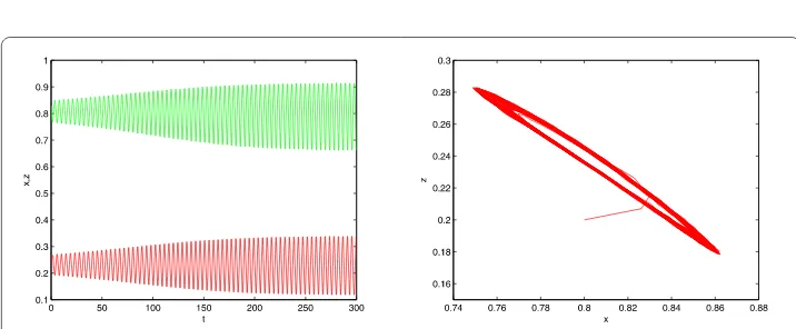
Figure 4The system has an asymptotically stable periodic orbit nearτ1for (μ1,μ2) = (0.11, 0.10). The green
line representsx, the red line representsz. Waveform diagram for variable ofx,z(left). Phase diagram for variable (x,z) (right)
–0.0007235 – 0.002548i, d21 = –0.008275, d22 = –0.002301; the equilibrium point is (0.8075, 0.2307), andτ1= 1.6735. For smallμ, we obtaink3= 0.
5 Conclusions
In this article, we have discussed the Hopf-zero bifurcation of Oregonator oscillator with delay. We thoroughly analyze the distribution of the eigenvalues of the corresponding characteristic equation and find some specific conditions ensuring that all the eigenval-ues have negative real parts. We also can discover the factors that make system (1.2) un-dergo a Hopf-zero bifurcation at equilibrium (x+,z+). Meanwhile, by using the normal form method and the center manifold theorem we have derived the normal form of the reduced system on the center manifold and discussed the Hopf-zero bifurcation with pa-rameters in system (1.2). Besides, we have obtained bifurcation diagrams and phase por-traits of system (3.13) whenB> 0 andB< 0, respectively. We also note that a saddle-node bifurcation and pitchfork bifurcation occur alongMandN, respectively, and a Hopf bifur-cation and a heteroclinic bifurbifur-cation occur alongHandS, respectively. Finally, numerical stimulations (see Figure 3, 4 and 5) have been given to illustrate the theoretical results.
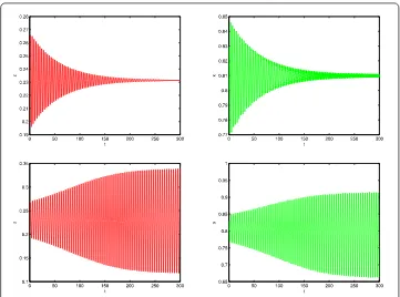
Figure 5Waveform diagram for variable ofx,z. The first two figures show that whenτ= 1.50 <τ10, the
system is stable around the equilibrium point. Whenτ= 1.80 >τ10, the next two figures show that the
system is unstable around the equilibrium point
Acknowledgements
The authors wish to express their gratitude to the editors and the reviewers for the helpful comments.
Funding
This research is supported by the Heilongjiang Provincial Natural Science Foundation (No. A2015016).
Competing interests
The authors declare that they have no competing interests.
Authors’ contributions
The idea of this research was introduced by YC, LL and CZ. All authors contributed to the main results and numerical simulations and approved the final manuscript.
Publisher’s Note
Springer Nature remains neutral with regard to jurisdictional claims in published maps and institutional affiliations.
Received: 9 September 2018 Accepted: 19 November 2018
References
1. Cao, X., Song, Y., Zhang, T.: Hopf bifurcation and delay-induced Turing instability in a diffusive lac operon model. Int. J. Bifurc. Chaos26(10), 1650167 (2016)
2. Chang, X., Wei, J.: Hopf bifurcation and optimal control in a diffusive predator–prey system with time delay and prey harvesting. Nonlinear Anal., Model. Control17(4), 379–409 (2012)
3. Chow, S.N., Li, C., Wang, D.: Normal forms and bifurcation of planar vector fields. Cambridge (1994)
4. Ding, W., Liao, X.F., Dong, T.: Hopf bifurcation in a love-triangle model with time delays. Neurocomputing260, 13–24 (2017)
5. Ding, Y., Jiang, W., Yu, P.: Hopf-zero bifurcation in a generalized Gopalsamy neural network model. Nonlinear Dyn.70, 1037–1050 (2012)
6. Faria, T., Magalhaes, L.T.: Normal forms for retarded functional differential equation with parameters and applications to Hopf bifurcation. J. Differ. Equ.122(2), 181–200 (1995)
7. Gazor, M., Sadri, N.: Bifurcation control and universal unfolding for Hopf-zero singularities with leading solenoidal terms. SIAM J. Appl. Dyn. Syst.15, 870–903 (2016)
9. Isaac, A.G., Jaume, L., Susanna, M.: On the periodic orbit bifurcating from a zero Hopf bifurcation in systems with two slow and one fast variables. Appl. Math. Comput.232, 84–90 (2014)
10. Jaume, L., Zhang, X.: On the Hopf-zero bifurcation of the Michelson system. Nonlinear Anal., Real World Appl.12, 1650–1653 (2011)
11. Jiang, H., Jiang, J., Song, Y.: Normal form of saddle-node-Hopf bifurcation in retarded functional differential equations and applications. Int. J. Bifurc. Chaos26, 1650040 (2016)
12. Jiang, W., Wang, H.: Hopf-transcritical bifurcation in retarded functional differential equations. Nonlinear Anal.73, 3626–3640 (2010)
13. Jiang, W., Wang, J.: Hopf-zero bifurcation of a delayed predator–prey model with dormancy of predators. J. Appl. Anal. Comput.7, 1051–1069 (2017)
14. Jimenez-Prieto, R., Silva, M., Perez-Bendito, D.: Analytical assessment of the oscillating chemical reactions by use chemiluminescence detection. Talanta8(44), 1463–1472 (1997)
15. Kaplan, D.T., Glass, L.: In Understanding Nonlinear Dynamics. Springer, Berlin (1995) 16. Kuznetsov, Yu.: Elements of Applied Bifurcation Theory, 3rd edn. Springer, Berlin (2004)
17. Liu, Z., Yuan, R.: Zero-Hopf bifurcation for an infection-age structured epidemic model with a nonlinear incidence rate. Sci. China Math.60(8), 1371–1398 (2017)
18. Marsden, J.E., Sirovich, L., John, F.: Nonlinear Oscillations, Dynamical System, and Bifurcations of Vector Fields. Nonlinear Mathematical Sciences, vol. 42 (2002)
19. Rodrigo, D., Jaume, L.: Zero-Hopf bifurcation in a Chua system. Nonlinear Anal., Real World Appl.37, 31–40 (2017) 20. Song, Y., Jiang, J.: Steady-state, Hopf and steady-state-Hopf bifurcations in delay differential equations with
applications to a damped harmonic oscillator with delay feedback. Int. J. Bifurc. Chaos22, 1250286 (2012) 21. Takens, F.: Lecture Notes in Math, vol. 3, pp. 56–78. Springer, Berlin (1981)
22. Tian, X., Xu, R.: The Kaldor–Kalecki stochastic model of business cycle. Nonlinear Anal., Model. Control16(2), 191–205 (2011)
23. Wang, H., Wang, J.: Hopf-pitchfork bifurcation in a two-neuron system with discrete and distributed delays. Math. Methods Appl. Sci.38(18), 4967–4981 (2015)
24. Wang, Y., Wang, H., Jiang, W.: Hopf-transcritical bifurcation in toxic phytoplankton–zooplankton model with delay. J. Math. Anal. Appl.415, 574–594 (2014)
25. Wu, X., Wang, L.: Zero-Hopf bifurcation for van der Pol’s oscillator with delayed feedback. J. Comput. Appl. Math.235, 2586–2602 (2011)
26. Wu, X., Wang, L.: Zero-Hopf bifurcation analysis in delayed differential equations with two delays. J. Franklin Inst.354, 1484–1513 (2017)
27. Wu, X., Zhang, C.R.: Dynamic properties of the coupled Oregonator model with delay. Nonlinear Anal., Model. Control
18, 359–376 (2013)
28. Yang, J., Zhao, L.: Bifurcation analysis and chaos control of the modified Chua’s circuit system. Chaos Solitons Fractals
77, 332–339 (2017)
![Figure 1 When B < 0, the bifurcation diagrams and phase portraits of system (3.13) (see [18])](https://thumb-us.123doks.com/thumbv2/123dok_us/940577.1114544/18.595.117.476.310.519/figure-b-bifurcation-diagrams-phase-portraits.webp)