R E S E A R C H
Open Access
Localization based on standard wireless
LAN infrastructure using MIMO-OFDM channel
state information
Tanee Demeechai
1*, Pratana Kukieattikool
1, Thang Ngo
2and Tae Gyu Chang
2Abstract
An indoor localization method using multiple input, multiple output orthogonal frequency division multiplexing (MIMO-OFDM) channel state information (CSI) is proposed as a method that can be implemented on wireless local area networks of a current standard without affecting their protocol structures and that does not require a training process for adaptation to indoor environments. In the proposed method, the CSI obtained by the MIMO-OFDM receivers of all access points upon successful reception of a data packet from a mobile terminal (MT) is processed in order to determine the location of the MT. The proposed method analyzes the multipath effect that appears in the CSI as multiple complex sinusoids by using the matrix pencil method in order to extract only terms that are contributed by direct paths from the MT to the access points. Localization is achieved using the direct-path terms on the basis of the maximum likelihood principle.
Keywords: Indoor localization, MIMO-OFDM, Channel state information, Multipath propagation, Matrix pencil method, Maximum likelihood principle
1 Introduction
Indoor localization is a hot research topic in the field of wireless communication owing to its capability to provide a wide range of location-based services for increasingly ubiquitous smart mobile devices. For indoor environ-ments, wireless local area network (WLAN) technology based on the IEEE 802.11 standards is widely employed around the world for providing data connections to mobile devices. Therefore, this paper focuses on indoor localization methods based on WLAN technology. Specif-ically, the purpose of this paper is to propose a localization method that can be implemented using the infrastruc-ture of a WLAN without affecting its protocol strucinfrastruc-ture. The proposed method will simultaneously exploit and be constrained by WLAN characteristics whereby WLANs are trending toward asynchronous networks of multi-ple input, multimulti-ple output orthogonal frequency division multiplexing (MIMO-OFDM) access points (APs) [1].
*Correspondence: [email protected]
1National Electronics and Computer Technology Center (NECTEC), National Science and Technology Development Agency (NSTDA), 112 Thailand Science Park, Phahonyothin Road, Pathum Thani 12120, Thailand
Full list of author information is available at the end of the article
Although many studies have investigated localization [2–6], it is not straightforward to apply their results to the problem of interest without requiring dedicated infras-tructure or affecting the WLAN protocol sinfras-tructure. A few localization methods based on the IEEE 802.11 standards have been proposed in the literature [7–9] and imple-mented commercially. However, most of these methods use the received signal strength indicator (RSSI) as data for location determination [7, 8]. The use of the RSSI usu-ally requires a disincentive process of measurement-based training for adaptation to ever-changing environments because the RSSI is very sensitive to both large-scale shadowing and small-scale multipath fading prevalent in indoor environments. Recently, a method that uses chan-nel state information (CSI) available through a network interface card [10] has been proposed [9]. Compared to the RSSI, the CSI is less sensitive to multipath fad-ing. Nevertheless, the method proposed in [9], which is based on single-antenna APs, requires a disincentive measurement-based training process. The method pro-posed in the present paper uses the CSI obtained by the MIMO-OFDM receiver of each AP as data for location determination, without any measurement-based training
process for adaptation to ever-changing environments. The details of the proposed method are described in subsequent sections.
2 Proposed localization method
According to the proposed method, the CSI obtained by the MIMO-OFDM receivers of all APs upon successful reception of a data packet from a mobile terminal (MT) is processed in order to determine the location of the MT. We assume that the MT uses only one antenna, i.e., one spatial stream, for transmitting the data packet for localization. Therefore, the packet’s preamble part for estimating the CSI by the OFDM receiver of each AP will consist of only one VHT-LTF (see [1], Fig. 22–4). It may be noted that, while the standard [1] defines four OFDM sig-nal models, classified according to the bandwidth as the 20-, 40-, 80-, and 160-MHz models, the duration of the VHT-LTF symbol equals 4μs including the 800-ns guard interval for all the models.
The localization method involves removing multipath reflection components in the CSI and searching for the best location on the basis of a likelihood metric. Because removing multipath reflection components in the CSI is an important step, the characteristics of indoor multi-path propagation and the CSI are discussed first; then, the algorithm of the proposed method is described in detail.
2.1 CSI from MIMO-OFDM receivers as location information
The CSI is always required for data demodulation in an OFDM receiver. Therefore, a receiver can provide the CSI at no overhead [10]. The CSI is represented by the chan-nel frequency response (CFR) for the set of used OFDM subcarriers. As radio wave propagation in indoor environ-ments is subjected to multipath characteristics, we may characterize the CFR as follows. Assuming that the anten-nas of an AP are closely located, the CFR estimated by the receiver of theq-th AP for them-th antenna andk-th subcarrier can be expressed by
Hk,m,q= NP−1
n=0
hn,qe−j2π(f0+kB/N)(tq+tn,m,q)+wk,m,q, (1)
whereNPis the number of paths in the channel model,hn,q is the complex amplitude of then-th path for theq-th AP, f0is the carrier frequency,tn,m,qis the propagation delay associated with then-th path between the MT antenna and them-th antenna of theq-th AP,Bis the OFDM sig-nal bandwidth,B/N is the OFDM subcarrier spacing,tq is the time shift introduced by the OFDM time synchro-nizer of the receiver, and wk,m,q is the estimation error that is assumed to behave as additive white Gaussian noise (AWGN). Note that a perfect OFDM time synchronizer
only needs to force the time shifttq to be well within a tolerance supported by the OFDM guard interval [11]. In other words, with a guard interval length oftg, the time shift is required to ensure that the effective delay of the shortest path is non-negative (tq +minn,m(tn,m,q) ≥ 0) while the effective delay of the longest path does not ex-ceed the guard interval length (tq+maxn,m(tn,m,q)≤tg). Therefore,
0≤tq+tn,m,q≤tg,∀(n,m). (2)
This uncertainty oftqis another source of variation of the CSI, which must be properly treated when the CSI is used for localization.
In this study, the AP antennas are closely located as an array with spacing between elements of the order of half wavelength. Therefore, the differences between the prop-agation times to the AP antennas for the same path man-ifest themselves as approximately frequency flat phase difference terms, i.e., (1) can be approximately expressed by ber of antennas in the antenna array for theq-th AP, and φn,m,q=2πf0(tq+tn,m,q−tn,q). Note that the phase terms
φn,m,q, 1≤m≤Mq, obey
∀m
φn,m,q=0 (4)
and share a relationship that depends on the antenna array geometry for theq-th AP and the angle of arrival (AOA) to the array from then-th path. In what follows, we shall assume that the terms in (3) have been sorted according to time delays such thattn1,q≤tn2,qifn1≤n2. Further, it may be noted that (2) becomes
0≤tn,q≤tg,∀n. (5)
We may then rearrange (3) as
Hk,m,q= NP−1
n=0
gn,qe−j(2πBtn,qk/N+φn,m,q)+wk,m,q, (6)
2.2 Proposed algorithm
The proposed algorithm consists of two major steps. The first step is to obtain CFRs that are effective for local-ization by minimizing irrelevant contributions from mul-tipath reflection and the uncertainty of the OFDM time synchronizer. The second step is to search for the best location on the basis of a likelihood metric.
2.2.1 Obtaining an effective CFR
To minimize irrelevant contributions from multipath reflection and the uncertainty of the OFDM time synchro-nizer in the CFR for them-th antenna of theq-th AP, we aim to obtain an effective CFR modeled by
Gm,q=g0,qe−jφ0,m,q+wm,q, (7)
wherewm,qdenotes the average ofwk,m,qacross k. Note that the effective CFR consists of the contribution from the shortest path and additive noise. Therefore, the effec-tive CFR will carry information of the MT location if the shortest path is actually the direct path. Hence, the main assumption of the proposed algorithm is that direct paths between the MT and the APs exist with consider-able amplitudes compared to the amplitude of the additive noise.
In the proposed algorithm, the effective CFRs for an AP are obtained by first obtaining reflection-rich CFRs for contiguous subcarriers from the CSI, then obtain-ing parameters of the sinusoids in the reflection-rich CFRs, and finally transforming the reflection-rich CFRs to obtain the result.
Obtaining a reflection-rich CFR for contiguous
sub-carriers According to the underlying standards [1], a
CFR can be obtained from the CSI only for used OFDM subcarriers that are discontiguous. The proposed algo-rithm obtains the CFR for contiguous subcarriers by sim-ply using linear interpolation to compute the CFR for unused subcarriers whenever they are between two used subcarriers. The linear interpolation method is clearly simple, but we consider whether it can effectively preserve the slow-oscillation characteristics of the shortest-path sinusoid. Hence, according to the standard signal models [1], the resulting CFR is contiguous for−K ≤ k ≤ K, where the values ofKfor the 20-, 40-, 80-, and 160-MHz signal models are 28, 58, 122, and 250, respectively.
Obtaining parameters of sinusoids A sinusoid as a
function ofk, expressed byaejωk, is characterized by its frequencyωand its complex amplitudea. To estimate the frequencies of all the sinusoids in the CFRs of the q-th AP, we adopt the matrix pencil method (MPM) [12, 13] because this constant amplitude multiple-sinusoid esti-mation problem is equivalent to the direction-of-arrival estimation problem with fully coherent sources, which
is directly addressed by the MPM . Moreover, the MPM method has been shown to be the most suitable method among various super-resolution methods [13].
Following [13] with our own notations, we may detail the estimation procedure as follows. According to [13], a snapshot of data is a sequence of limited samples of the observation. Therefore, from the CFR data of theq-th AP, we haveMqsnapshots of data, with each snapshot con-taining 2K+1 samples. Accordingly, the input data matrix is formed as
Y=[Y1 Y2 · · · YMq] , (8)
whereYm denotes the Hankel matrix for them-th snap-shot. Thus, the pencil parameter. In [13], it is stated that if the value ofLis selected from a certain range, the variance of the estimation results will be minimal. Such a range depends on the snapshot size, which is then translated to our case as
(2K+1)/3≤L≤(2K+1)/2. (10) Here, the value ofLwill be selected on the basis of the simulation results for this range.
Then,YRis obtained by reducing the rank ofYtoNU, which is the number of significant sinusoids in the data. This is based on singular-value decomposition as follows. Suppose thatYcan be expressed as
Y=USVH, (11)
where(·)Hdenotes the matrix conjugate and transpose,U
andVare unitary matrices, composed of the eigenvectors ofYYHandYHY, respectively, andSis a diagonal matrix containing the singular values ofY. Then,
YR=USRVH, (12)
complex analytically, the value selected in this paper will be based on a simulation study.
Then, the frequency values of the NU sinusoids are obtained from YR as follows. First, the eigenvalues of
Y+1Y2 are evaluated, where (·)+ denotes the Moore-Penrose pseudoinverse, andY1andY2are matrices of size
(2K−L+1)×MqL, obtained by deleting the last and first rows of YR, respectively. Then, theNU frequency values
ω0,ω1, . .,ωNU−1are obtained as the angles of the obtained NUeigenvalues.
Suppose that theNUfrequency valuesω0,ω1, . .,ωNU−1 just obtained have been already sorted in descending order. In addition, consider for simplicity that all theNP paths in (6) have clearly distinctive delays and consider-able amplitudes compared to the amplitude of the noise. Then,NU is an estimate ofNP. In addition, theNU fre-quency values can be considered as they are related with the effective path delaystn,qbyωn = −2πBtn,q/N. Then, the corresponding complex amplitudes an,m, 0 ≤ n <
NU, that estimate gn,qe−jφn,m,q are obtained by applying the conventional linear least-squares method [14] to the problem:
Transforming a reflection-rich CFR Recall that NU
denotes the number of significant sinusoids for the fre-quency estimation. Then,NU−1
n=1 an,mejωnk approximates (6), where the terms of the shortest path and the AWGN are ignored, i.e.,
Therefore, the effective CFR for the m-th antenna is obtained by first computing the left-hand side of (15), then translating the frequency of the remaining shortest-path term to zero, and finally averaging the result over the frequency domain, i.e.,
2.2.2 Search for the best location
Searching for the best location involves the computation of likelihood-based metrics for locations of interest, and it is equivalent to maximizing the likelihood over the locations. The likelihood to be maximized is defined by
u(ζ)=f(Gm,q;∀(m,q)|ζ,g0,∗q;∀q), (18)
wheref(·)denotes the probability density function (PDF), ζ denotes the location, and g∗0,q,∀q, are g0,q,∀q, that jointly maximizef(Gm,q;∀(m,q)|ζ,g0,q;∀q). Assume that the CSI data have been scaled such that the variances of wk,m,q,∀(m,q), are the same. Note that such scaling requires the average noise power or signal-to-noise ratio of every receiver chain to be estimated. However, as the information is generally required also by the MIMO-OFDM receiver, obtaining the information should not involve any overhead. Then, based on (7) and because wm,q,∀(m,q), are zero mean independent and identical circularly symmetric complex Gaussian random variable with meanμand varianceσ2,λis the wavelength of the radio-frequency carrier,rm(ζ ),qis the distance fromζ to the
m-th antenna of theq-th AP, and¯rq(ζ ) = m=Mq1r(ζ )m,q/Mq. Then, it can be shown that
arg max
Then, to determine the best location, the metric defined as
is computed for every location of interest, and the best locationζ∗is obtained ass(ζ∗)=maxζs(ζ).
2.3 Some remarks
2.3.1 AOA-based localization
s(ζ)=∀qsq(ζ), wheresq(ζ)= |∀mGm,qej(2π/λ)r
(ζ )
m,q|2. The metric contributed by the data of an AP has an inter-esting property that may be described as follows. Note that the metric sq(ζ) can be equivalently expressed by
sq(ζ) = |∀mGm,qej(2π/λ)[r conclude that the metric contributed by the data of an AP contains information of the AOA to the AP.
The usefulness of the effective CFR obtained by (16) may be noted as follows. Thus far, we have assumed that the direct path exists and all paths also have distinctive delays. However, paths can actually have indistinguishable delays. Then, a problem could arise when some scattered paths of considerable amplitudes have delays close to the delay of the direct path, while they also have AOAs con-siderably different from that of the direct path. In this case, the effective CFR will possibly contain also the AOA information of the scattered paths that can degrade the location estimation of the proposed algorithm. There-fore, the proposed algorithm requires significant scattered paths with delays close to the delay of the direct path to also have AOAs close to the AOA of the direct path. This could be realistic if the placement of the AP antenna array is not close to any significant reflective materials. Such placement also seems to be a good practice for other AOA-based localization systems.
2.3.2 Effect of MT velocity
It may be interesting to assess the effect of the MT veloc-ity on the performance of the proposed algorithm. In this regard, we consider that there are two issues caused by MT movement that may affect the performance. One issue is the location shift of the MT that may change the real multipath configuration of the channel during the OFDM training symbol. The other issue is the Doppler shift of the direct-path term in the estimated CSI. The location shift should be of no concern because the dura-tion of the training symbol is just 4μs, which means that a moving speed of 900 km/h is required to observe a loca-tion shift of 1 mm. The 1-mm shift does not seem to significantly change the multipath configuration, and the 900-km/h speed is infeasible in indoor environments.
Regarding the Doppler shift, it should be noted that movement of the MT during a packet transmission would cause a direction-dependent spectral shift of the radiating wave. Hence, the spectral shift of one transmission path arriving at the receiver could be different from the spec-tral shifts of other paths. This effect is not as simple as that of the local oscillator frequency offset between the trans-mitter and the receiver, where the effect is equivalent to causing identical spectral shifts for all paths. However, the
direction-dependent spectral shifts could only change the phases of the sinusoidal terms in (6) and therefore could not affect the frequency estimation of the MPM. In addi-tion, the spectral shift of the direct-path term could only rotate g0,q in (6) through a certain angle and therefore could not change the MT location information inφ0,m,q, 1≤m≤Mq.
However, the Doppler shift is known to cause inter-carrier interference in OFDM data detection. It will also affect the CSI estimation that is conventionally based on detecting the data carried by the training symbol. For a successfully detected data packet, we can expect that such interference is insignificant. Therefore, in this paper, we assume that the effect is negligible. Nevertheless, we believe that it merits a detailed analysis that should be conducted in a separate study.
2.4 CRLB for two-dimensional systems with linear-type arrays
For benchmarking the performance of the location esti-mators based on (7), we obtain the Cramer-Rao lower bound (CRLB) [15], which is the variance of the estima-tion error of a minimum variance unbiased estimator. This is done on the basis of the following considerations. First, we model the observation of the estimator as a real vector:
X=
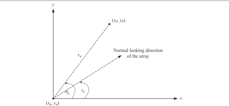
Fig. 1Illustration of geometrical reference model. Illustration of geometrical reference model of (x0,y0), (xq,yq), (rq,θq), andγq
asγq. For example, if the array elements of theq-th AP are placed along thex-axis in Fig. 1,γqwill beπ/2. Then, assuming that the spacing between the antenna elements in each array is d andrq >> d, φ0,m,q,∀(m,q), can be approximated by
φ0,m,q= 2π
λ (m−(Mq+1)/2)dsin(θq−γq). (24) Based on [15], the CRLB can be computed by
CRLB(ζ)ˆ =[I−1]1,1+[I−1]2,2, (25)
where [K]i,jdenotes the(i,j)element of matrixKandIis the Fisher information matrix:
[I]i,j= 2 σ2
∂μT
∂ui ∂μ ∂uj
, (26)
where μ is the mean of X, and (u1,u2, ..,u2Q+2) =.
(x0,y0,|g0,1|,∠g0,1, ..,|g0,Q|,∠g0,Q). However, following [16], the CRLB may be also computed by
CRLB(ζ)ˆ =[I−e1]1,1+[I−e1]2,2, (27)
where Ie is the equivalent Fisher information matrix obtained as follows. Let
I=
A B
BT C
, (28)
where the sizes of matricesA,B, andCare 2×2, 2×2Q, and 2Q×2Q, respectively. Then,Iecan be computed by
Ie=A−BC−1BT. (29)
Noting that ∂θq/∂x0 = −(sinθq)/rq and ∂θq/∂y0 =
(cosθq)/rq, we then apply these two relations and (22), (23), and (24) to derive the elements of A, B, and C.
Accordingly, after arranging the terms, we obtain B as a zero matrix, and therefore, Ie = A, which can be expressed by
Ie= 1 σ2
Q
q=1 |g0,q|2
Mq(M2q−1)
6
2πdcos(θ
q−γq)
λrq
2
p(θq)p(θq)T,
(30)
where
p(θq)=sin(θq) −cos(θq)T. (31)
We may use (27) and (30) to compute the CRLB as a function ofg0,q, 1 ≤ q ≤Q, which are random variables. In this paper, by considering such variability, the CRLB is then obtained by averaging the computed CRLBs across the simulated values of{g0,q|1≤q≤Q}.
3 Numerical results and discussions
3.1 Multipath propagation model
In this paper, we estimate the performance of the pro-posed algorithm on the basis of computer simulation using statistical indoor channel models. In addition, because our algorithm is AOA-based, we require a rele-vant channel model to provide specifications of the AOA characteristics in addition to the power delay profile of the multipath. As we find that only the IEEE 802.11 TGn channel models [17] are available in detail and meet our requirements, we base our performance evaluation on only such models.
tap representing the contribution of scattered paths of the same delay. The delay taps are grouped into clusters such that scattered paths within the same cluster possess the same random characteristics of the AOA to the receiver. In other words, the AOAs of scattered paths of a clus-ter are obtained as follows. First, the mean AOA is drawn from a uniform distribution over [0,2π). Then, the AOA of each scattered path is drawn from a Laplacian distribution according to the obtained mean and the angular spread (AS), i.e., the standard deviation, specific to the cluster. The amplitude of a scattered path is a complex Gaussian random variable, with the magnitude being a Rayleigh dis-tribution. The number of clusters, power delay profile, and AS of each cluster are specific to model subtype, e.g., the number of clusters is three for model D. The total received power in an NLOS model is also subjected to path loss, which includes a log-normal shadowing effect and is specific to the model subtype. The TGn channel modeling also provides a line-of-sight (LOS) model for each model subtype, which is relevant to our case where the localization algorithm requires the existence of LOS. In a TGn channel model, an LOS model of a subtype is simply obtained by adding an LOS component to the first arriving tap of the corresponding NLOS model. However, the addition is done according to a first-tap k-factor, i.e., the ratio of the LOS power to the average power of the NLOS first tap, which is specific to the model subtype. The TGn channel modeling does not use a large first-tap k-factor for any model subtype because changing from the NLOS model to the LOS model of the same subtype will slightly reduce the root-mean-square (RMS) delay spread of the channel (see Table 1).
However, we note that the described LOS model con-sists of LOS and NLOS parts, with the first tap of the NLOS part being set to have the same delay as (but arbitrarily different AOA from) the LOS. This seems to be unrealistic if the placement of the AP antenna array is not close to any significant reflective materials. Such placement seems to be also a good practice for other AOA-based localization systems. Assume that such place-ment has been done successfully for every array, although
Table 1NLOS and LOS characteristics of models D and E of [17]
Model D Model E
First-tap k-factor (dB) NLOS −∞ −∞
LOS 3 6
RMS delay spread (nm) NLOS 50 99
LOS 47 95
Maximum delay spread (nm) NLOS 390 730
LOS 390 730
absorptive materials may be required in some cases. Then, it would be more realistic if a scattered path with a delay close to that of the LOS also had its AOA statistically close to that of the LOS. Accordingly, we modify the TGn chan-nel models for our purpose by (i) setting the mean AOA of the NLOS first tap to equal the AOA of LOS and (ii) introducing a new parameterσ0 as the AS of the NLOS first tap. The impact of this parameter on the algorithm performance will be studied by simulation.
The TGn channel models include six model subtypes with RMS delay spread in the range of 0 to 150 ns. We use the LOS models D and E in this paper because accord-ing to [18], the associated delay spreads are representative of typical office environments for model D and typical large open spaces and office environments for model E. In addition, such environments are expected to be tar-gets of a wide range of indoor location-based services. The characteristics of the two models in terms of the first-tap k-factor, the RMS delay spread, and the maximum delay spread (tNP−1,q−t0,q) are summarized in Table 1, while additional details can be found in [17]. Note that each LOS model is multipath-rich while having a direct path that is nondominant because changing from the NLOS model to the LOS model of the same subtype can just slightly reduce the RMS delay spread of the channel.
3.2 Common assumptions and search method
The performance of the proposed method is evaluated with geometrical assumptions as shown in Fig. 2, illus-trating the region of interest for localization, which is a square having an area of 400 m2and the normal looking directions of the antenna arrays of four APs located at the corners of the square. Each antenna array is of linear type with half-wavelength spacing between elements. A carrier frequency of 5 GHz is assumed. In addition, an antenna gain of 0 dB is assumed for the MT antenna as well as for each array element of an AP. Further, it is assumed that the variance of the CSI estimation error depends only on the system noise, i.e., E|Hk,m,q−wk,m,q|2]/E[|wk,m,q|2
equals the average signal-to-noise ratio per OFDM sub-carrier. Regarding the OFDM signal models [1], we will consider only the 40-, 80-, and 160-MHz models, as they should be sufficient for demonstrating the performance with regard to the bandwidth.
Fig. 2Illustration of geometrical simulation assumptions. The 400-m2region of interest for localization and the normal looking directions of the
antenna arrays of four APs located at the corners
grid-point spacing in meters for then-th round. Note that the grid-point spacing for the last round, representing the effective resolution of the search space, is 10−2m.
3.3 Selection of algorithm parameters
The performance of the proposed algorithm depends on its parameters L andρ. We realize that obtaining opti-mal values of the parameters may require a separate elaborate study. In this paper, we only select certain val-ues for demonstrating the basic working performance of the proposed algorithm and for comparing the proposed algorithm with previous methods. This is done for each standard signal model [1] as follows.
First, we select a tentative value ofLto be the middle value of the range (10). Therefore, the selected values for the 40-, 80-, and 160-MHz OFDM signal models are 49, 102, and 209, respectively.
Then, a tentative value ofρ is selected from the sim-ulation results as shown in Fig. 3. The results show the root-mean-square error (RMSE) versus ρ with OFDM signal bandwidth (B) and number of antennas per AP (Mq = M,∀q) as parameters. The RMSE is obtained from 1000 independent samples, based on the following assumed typical conditions. The MT transmitted power is 10 dBm, the AP receiver noise figure (NF) is 4 dB, and the LOS model D is used withσ0 = 4°. In addition, the MT is uniformly and randomly located in the 400-m2region, except the locations that are close to the center of an antenna array by less than 1 m. All the RMSE values shown
in the figure are based on same test data, defined by the drawn MT locations and channel characteristics. Accord-ing to the results, the selected values ofρare 1/32 for the 40- and 80-MHz models and 1/16 for the 160-MHz model, as they represent a rough approximation of the optimal values for the assumed conditions.
Then, we iterate the simulation experiments by fixing the value ofρ to the tentative one and performing sim-ulations for evaluating the performance in terms of L. According to the results, the performance does not vary significantly withL. Therefore, the tentative values ofL andρstated above are adopted in this paper.
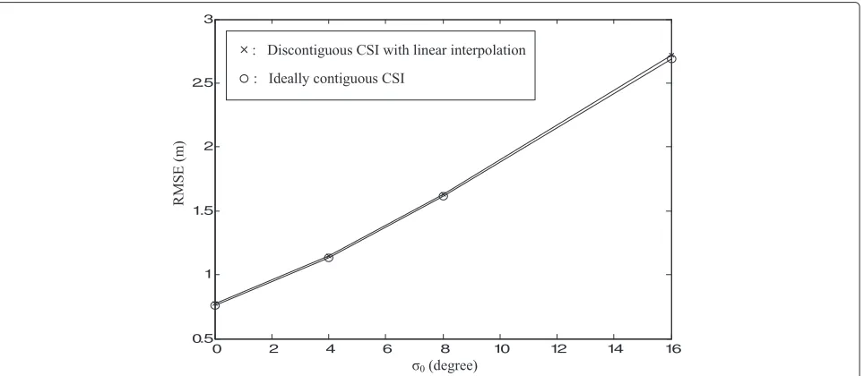
3.4 Implications ofσ0and CSI interpolation
Fig. 3Average localization error in terms ofρ. Root-mean-square error versusρwith OFDM signal bandwidth and number of antennas per AP as parameters
with linear interpolation leads to slightly worse perfor-mance. Hence, we may conclude that linear interpolation is effective in mitigating the problem of CSI discontigu-ity in the proposed algorithm. The results also show that the RMSE values whenσ0 = 0°, 4°, 8°, and 16° for both cases are around 0.7, 1.1, 1.6, and 2.7 m, respectively. Hence, controllingσ0to be small based on the placement of the antenna arrays as mentioned in Section 3.1 is very important for realizing good performance of the proposed algorithm.
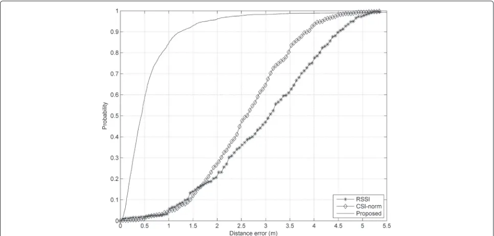
3.5 Comparison with other methods
The performances of the proposed method, the RSSI-based method [8], and the CSI-RSSI-based method [9] were compared under the same statistical channel conditions. The CSI-based method [9] and the RSSI-based method are similar but differ in terms of the observation data that they use. The RSSI-based method uses the RSSI as observation data, whereas the CSI-based method [9] uses a norm computed from the CSI as observation data. We will refer to the RSSI-based method [8] and the CSI-based
method [9] as the RSSI method and the CSI norm method, respectively. Both methods require the localization algo-rithm to be trained before use or testing. In the training process, usually referred to as fingerprinting, the PDF of the observation data conditioned on the MT location is obtained from the training data for each reference loca-tion. In the use phase, the location is determined as a weighted average of the reference locations according to the observation data and the trained model. For the per-formance comparison, the LOS models D and E are used with the following simulation conditions. The MT trans-mitted power is 10 dBm, the AP receiver NF is 4 dB, and each LOS model hasσ0 =4◦. In addition,B=160 MHz andM=2. The MT locations for testing are rectangular grid points spanning the 400-m2region with a grid-point spacing of 1 m, except for the center points of the four antenna arrays. The set of reference locations for the RSSI and CSI-norm methods is the same as the set of MT loca-tions for testing. Because the RSSI and CSI-norm methods assume observation data from a single antenna, the RSSI and CSI-norm averaged across the antennas in the array are respectively used as the observation data for the two methods in this paper. The training data for each reference location consist of 500 independent samples of the obser-vation data, while the test data for each grid point consist of 10 other independent samples.
Figures 5 and 6 show the results of the cumulative distribution function (CDF) according to models D and E, respectively. It can be noted that the proposed algo-rithm clearly outperforms the other two methods in both
channel models. Note that the RSSI and CSI-norm meth-ods are not generally designed to model both small-scale and large-scale fading effects. They are designed to model only the variabilities of small-scale fading conditioned on a fixed large-scale fading condition because when a sig-nificant object moves in the environment and changes the large-scale fading condition, the methods usually need to be retrained for maintaining the performance. In the simulation environment of this study, different samples of observation data correspond to totally inde-pendent fading conditions. Therefore, the two methods cannot perform well in this simulation experiment. The figures also show that the performance of the proposed method improves when changing from model D to model E, possibly because of the stronger LOS component in model E.
3.6 Effect of infrastructure conditions
Figure 7 shows the results of the localization performance in terms of the signal-to-noise condition, signal band-width, and number of antennas per AP. The localization performance is evaluated with the same assumptions as in Section 3.3, except thatLandρare set to be the selected values and the MT transmitted power is varied over the range of−20 to 20 dBm. All the RMSE values shown in the figure are based on the same test data, defined by the drawn MT locations and channel characteristics. The figure shows that the localization performance improves with increasing MT transmitted power, but the improve-ment is saturated when the power increases over around
Fig. 6Performance comparison according to channel model E. CDF of localization errors for the RSSI, CSI-norm, and proposed methods according to channel model E
10 dBm. We believe that the performance saturation could be mainly due to residual contributions from scattered paths that still remain in the effective CFR. Note that we could expect such contributions to be smaller by having richer observation data for the multiple-sinusoid param-eter estimation process of the proposed algorithm. This is supportive of the results shown by the figure, where the saturated performance improves with increasingBor
M. The saturated performance, when the MT transmit-ted power equals 10 dBm, is summarized in Table 2. The table lists numerical values of the RMSE in meters and also in percent maximal length of a straight line within the localization region, in order to illustrate how the errors are related to the dimension of the localization region. Note that the maximal length is considered to be 20√2 m. Comparing the performance improvement as a result of
Table 2Localization performance in terms ofBandMwhen the MT transmitted power is 10 dBm, expressed as root-mean-square error in meters and also in percent maximal length of a straight line within the localization region
M=2 M=4
B(MHz)
40 3.9 m; 13.79 % 2.8 m; 9.90 %
80 2.0 m; 7.07 % 1.8 m; 6.36 %
160 1.2 m ; 4.24 % 1.1 m ; 3.89 %
changing fromM = 2 toM = 4 for the three cases of Bshown in the table, we can see that the improvement decreases with increasingB.
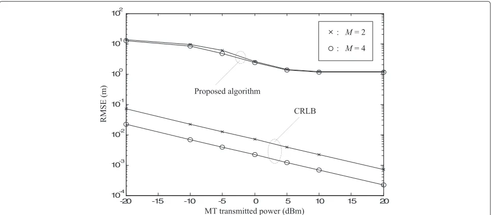
Figure 8 compares the results of Fig. 7 and the CRLB when B =160 MHz. The important points to be noted are as follows. The CRLB performance always improves steadily with increasing MT transmitted power. The per-formance of the proposed algorithm is much worse than that of the CRLB in all the cases. This large perfor-mance gap is expected because the CRLB here is based on the observation data modeled by (7), which is free of scattered-path contributions, and the CRLB result corre-sponds to an optimal unbiased estimator. The source of impairment of the CRLB results is only the AWGN.
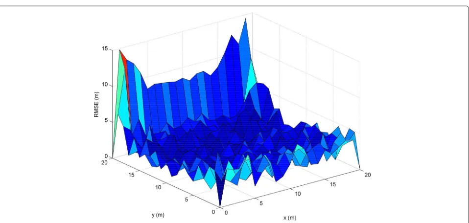
It is also interesting to see how the proposed method performs in terms of the MT location and the number of usable APs. Figures 9, 10, 11 and 12 show the simulation results with the same assumptions as in Section 3.5, except that the test data for each grid point here consist of 30 independent samples and only model D is used.
It can be noted from Fig. 9 that the 90 % confidence level error bound, i.e., the error when the cumulativeprobability
is 0.9, increases approximately from 1.2 to 1.6 and 3.5 m when the number of usable APs is reduced from 4 to 3 and 2, respectively. The performance seems to degrade steadily if the number of usable APs is greater than two. However, the performance with two APs is still better than the performances of the RSSI and CSI-norm methods with four APs, as shown in Fig. 5, from which we may note that the 90 % confidence level error bounds are around 4.5 and 3.8 m for the RSSI and CSI-norm methods, respectively. For the proposed method, the preferable number of usable APs seems to be three or greater, while having only two usable APs may still be viable in some applications.
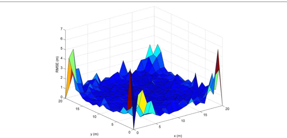
Regarding the localization performance in terms of the MT location, it is interesting to note from Fig. 10 that the RMSE is locally large for locations on the line connect-ing the two usable APs. This can be explained by notconnect-ing that the locations on such a line correspond to the case where the equivalent Fisher information matrix expressed in (30) is singular. Intuitively, the singularity indicates that the available information is not sufficient for esti-mation, i.e., the location information contribution in the observation data is not sufficient for deducing a location. Therefore, the localization performance in the singularity case here is extremely vulnerable to the AWGN. It may be noted from Figs. 11 and 12 that having more usable APs effectively relieves the singularity problem, especially for locations farther away from the two underlying APs. In contrast, having more usable APs is less effective in relieving the problem for locations close to an AP, possibly because the equivalent Fisher information matrix for such a location is largely dominated by only the contribution of that AP.
Fig. 9Performance in terms of the number of usable APs. CDF of localization errors in terms of the number of usable APs
4 Recommendations for further study
The purpose of this paper is to introduce a new algorithm for indoor localization and to demonstrate the poten-tial superiority of the proposed algorithm over previous approaches to the same problem. We believe that the issues listed below merit further investigation.
• Validation with real measurements: In this paper, the
localization performance of the proposed algorithm was evaluated on the basis of statistical indoor
channel models specifically obtained for
benchmarking data communication systems. It is much more relevant to evaluate the performance on the basis of real measurements or a statistical indoor channel model specifically obtained from real measurements for benchmarking AOA-based localization systems. Therefore, performance validation with real measurements is very important.
Fig. 11Average localization error in terms of the MT location based on three usable APs. Root-mean-square error versus MT location when only three APs located at (0,20), (20,20), and (20,0) m are usable
• Other super-resolution methods: Estimating the
frequencies of all the sinusoids in the CFRs plays a major role in obtaining an effective CFR for the proposed algorithm. Although the MPM is used in this paper because it directly addresses the problem of interest, we believe that other super-resolution methods should also be studied in this regard.
• Using a priori knowledge in estimation: In this paper,
estimating the parameters of all the sinusoids in the CFRs plays a major role in obtaining an effective CFR. Such estimation has been performed without
considering a priori knowledge about the parameters, i.e., their statistical models. Note that such knowledge may be used to improve the estimation performance
in general, as discussed in [16]. Applying such knowledge to the proposed algorithm is an interesting direction for further study.
• Optimal parameters for the algorithm: In this paper,
the values of the algorithm parametersLandρwere
selected for simply demonstrating the basic working performance of the proposed algorithm. Actually, the optimal values could depend on variable conditions of the radio channel and infrastructure. These effects are also worthy of further study.
• Problem of NLOS : In addition to bandwidth
availability and multiple-antenna configuration, an essential requirement for the proposed algorithm to work is the availability of LOS in the radio channel. In this regard, the availability required is just sufficient for triangulation. This requirement is the same as for the ultrawideband-based localization regime [19, 20]. Several methods for mitigating the problem of LOS availability have been presented in the literature. These methods are based on the detection of channel condition. By applying the detection of channel condition, we may simply ignore an AP if the detection result declares unavailability of LOS. We could then expect performance degradation on the basis of the results shown in Fig. 9, or encounter an outage if the number of usable APs is less than two. We note that the signal processing results obtained using the proposed method are employed as observation data for the detection of channel condition. However, a detailed study of such detection is beyond the primary scope of the present paper and it is therefore recommended for future work.
• AOA bias induced by diffraction: In the present
study, the effect of diffraction caused by building components, such as walls, is ignored. If not properly managed, this effect may degrade the performance of the proposed algorithm by introducing a bias into the AOA of a direct path, as well as the performance of the ultrawideband-based localization regime by introducing a bias into the time of arrival of a direct path. Therefore, further investigation is required to efficiently mitigate such a bias.
• MT velocity effect: As discussed in Section 2.3.2, a
detailed analysis of the effect of MT velocity on the localization performance should be carried out in a future study.
• Simple way to obtain the effective CFR : Note that
an,mobtained using the proposed algorithm by
solving (13) is an estimation ofgn,qe−jφn,m,q.
Therefore, according to (7),a0,mis also an estimation
ofGm,q. Then, it might be better to save computation
by usinga0,masGm,q, instead of obtainingGm,qfrom
(16). This issue also requires further investigation in
order to observe its possible effects on the localization performance.
5 Conclusions
A new localization method based on an asynchronous network of MIMO-OFDM access points was proposed. This method can be implemented on WLANs of a cur-rent standard without affecting their protocol structures. The method involves first obtaining effective CFRs, in which irrelevant contributions from scattered paths and the uncertainty of the OFDM time synchronizer are min-imal, and then searching for the most likely location. The proposed method does not require a training process for adaptation to ever-changing environments. The availabil-ity of direct paths is sufficient for triangulation, as in the ultrawideband-based localization regime. Further, signifi-cant scattered paths with delays close to the delay of the direct path are required to have AOAs close to the AOA of the direct path.
Competing interests
The authors declare that they have no competing interests.
Author details
1National Electronics and Computer Technology Center (NECTEC), National Science and Technology Development Agency (NSTDA), 112 Thailand Science Park, Phahonyothin Road, Pathum Thani 12120, Thailand.2School of Electrical and Electronics Engineering, Chung-Ang University, Seoul, South Korea.
Received: 15 July 2015 Accepted: 31 May 2016
References
1. IEEE Std 802.11ac - 2013, IEEE Standard for Information
Technology–Telecommunications and information exchange between systems–local and metropolitan area networks–specific requirements, Part 11: wireless LAN medium access control (MAC) and physical layer (PHY) specifications, Amendment 4: enhancements for very high throughput for operation in bands below 6 GHz. (The Institute of Electrical and Electronics Engineers, Inc., New York, NY, USA, 2013) 2. H Liu, H Darabi, P Banerjee, J Liu, Survey of wireless indoor positioning
techniques and systems. IEEE Trans. Syst. Man, Cybernetics–Part C: Appl. Rev.37(6), 1067–1080 (2007)
3. Z Farid, R Nordin, M Ismail, Recent advances in wireless indoor localization techniques and system. J. Comput. Netw. Commun.2013(185138), 1–12 (2013)
4. K Yu, I Sharp, YJ Guo,Ground-based wireless positioning, 1st edn. (Wiley, West Sussex, United Kingdom, 2009)
5. Y Zhao, K Liu, Y Ma, Z Li, An improved k-NN algorithm for localization in multipath environments. EURASIP J. Wireless Commun. Netw.2014(208), 1–10 (2014)
6. MB Zeytinci, V Sari, FK Harmanci, E Anarim, M Akar, Location estimation using RSS measurements with unknown path loss exponents. EURASIP J. Wireless Commun. Netw.2013(178), 1–14 (2013)
7. P Bahl, VN Padmanabhan, inIEEE INFOCOM. RADAR: an in-building RF-based user location and tracking system (The Institute of Electrical and Electronics Engineers, Inc, New York, NY, USA, 2000), pp. 775–784 8. M Youssef, A Agrawala, inProceedings of the 3rd International Conference
on Mobile Systems, Applications, and Services. The Horus WLAN location determination system (Association for Computing Machinery, New York, NY, USA, 2005), pp. 205–218
10. D Halperin, W Hu, A Sheth, D Wetherall, Tool release: gathering 802.11n traces with channel state information. ACM SIGCOMM Comput. Commun. Rev.41(1), 53 (2011)
11. TM Schmidl, DC Cox, Robust frequency and timing synchronization for OFDM. IEEE Trans. Commun.45(12), 1613–1621 (1997)
12. TK Sarkar, O Pereira, Using the matrix pencil method to estimate the parameters of a sum of complex exponentials. lEEE Antennas Propag. Mag.37(1), 48–55 (1995)
13. N Yilmazer, S Ari, TK Sarkar, Multiple snapshot direct data domain approach and ESPRIT method for direction of arrival estimation. Digital Signal Process18, 561–567 (2008)
14. GH Golub, CF Van Loan,Matrix computations, 4th edn. (Johns Hopkins University Press, Baltimore, MD, USA, 2013)
15. SM Kay,Fundamentals of statistical signal processing: estimation theory. (Prentice Hall, New Jersey, USA, 1993), p. 47
16. Y Shen, MZ Win, Fundamental limits of wideband localization: part I: a general framework. IEEE Trans. Inform. Theory.56(10), 4956–4980 (2010) 17. V Erceg, et al. IEEE P802.11 Wireless LANs: TGn channel models. IEEE
document 802.11-03/940r4. (The Institute of Electrical and Electronics Engineers, Inc, New York, NY, USA, 2004)
18. J Medbo, P Schramm. Channel Models for HIPERLAN/2 in Different Indoor Scenarios. ETSI/BRAN document no. 3ERI085B. (European
Telecommunications Standards Institute, Valbonne, FRANCE, 1998) 19. Z Sahinoglu, S Gezici, inIEEE Wireless and Microwave Technology
Conference. Ranging in the IEEE 802.15.4a standard (The Institute of Electrical and Electronics Engineers, Inc., New York, NY, USA, 2006) 20. M Losada, L Zamora-Cadenas, U Alvarado, I Velez, inIEEE International
Conference on Ultra-Wideband. Performance of an IEEE 802.15.4a ranging system in multipath indoor environments (The Institute of Electrical and Electronics Engineers, Inc., New York, NY, USA, 2011), pp. 455–459
Submit your manuscript to a
journal and benefi t from:
7Convenient online submission
7Rigorous peer review
7Immediate publication on acceptance
7Open access: articles freely available online
7High visibility within the fi eld
7Retaining the copyright to your article
![Table 1 NLOS and LOS characteristics of models D and E of [17]](https://thumb-us.123doks.com/thumbv2/123dok_us/939684.1114411/7.595.58.290.617.732/table-nlos-los-characteristics-models-d-e.webp)