Machine learning based dynamic frequency and bandwidth allocation in self organized LTE dense small cell deployments

R E S E A R C H

Open Access

Machine learning-based dynamic

frequency and bandwidth allocation in

self-organized LTE dense small cell

deployments

Biljana Bojovi´c

, Elena Meshkova

, Nicola Baldo

, Janne Riihijärvi

and Marina Petrova

Abstract

Self-organizing networks (SONs) are expected to minimize operational and capital expenditure of the operators while improving the end users’ quality of experience. To achieve these goals, the SON solutions are expected to learn from the environment and to be able to dynamically adapt to it. In this work, we propose a learning-based approach for self-optimization in SON deployments. In the proposed approach, the learning capability has the central role to perform the estimation of key performance indicators (KPIs) which are then exploited for the selection of the optimal network configuration. We apply this approach to the use case of dynamic frequency and bandwidth assignments (DFBA) in long-term evolution (LTE) residential small cell network deployments. For the implementation of the learning capability and the estimation of KPIs, we select and investigate various machine learning and statistical regression techniques. We provide a comprehensive analysis and comparison of these techniques evaluating the different factors that can influence the accuracy of the KPI predictions and consequently the performance of the network. Finally, we evaluate the performance of learning-based DFBA solution and compare it with the legacy approach and against an optimal exhaustive search for best configuration. The results show that the learning-based DFBA achieves on average a performance improvement of 33 % over approaches that are based on analytical models, reaching 95 % of the optimal network performance while leveraging just a small number of network measurements.

Keywords: Machine learning, Frequency allocation, Dense small cell deployment, Self-organized networks, LTE

1 Introduction

In recent years, the fourth generation (4G) mobile net-works have been rapidly growing in size and complex-ity. Operators are continuously seeking to improve the network capacity and the QoS by adding more cells of different types to the current deployments consisting of macro-, micro-, pico-, and femtocells. These heteroge-neous deployments are loosely coupled, increasing the complexity of 4G cellular networks. This increase in com-plexity brings a significant growth in the operational and the capital expenditures (OPEX/CAPEX) of the mobile network providers. To reduce these costs on a long-term

*Correspondence: [email protected]

1Centre Tecnològic de Telecomunicacions de Catalunya (CTTC), 08860 Castelldefels, Av. Carl Friedrich Gauss 7, Spain

Full list of author information is available at the end of the article

scale, operators are seeking network solutions that will provide automatic network configuration, management, and optimization and that will minimize the necessity for human interventions. In 2008, the next-generation mobile networks (NGMN) alliance recommended self-organizing networks (SONs) as a key concept for next-generation wireless networks and defined operator use cases in [1]. Shortly after, the SON concept was recognized by the Third-Generation Partnership Project (3GPP) as an essential functionality to be included in the long-term evolution (LTE) technology and consequently it was intro-duced into the LTE standard in [2]. SONs are expected to reduce the OPEX/CAPEX and to increase the capac-ity and the QoS in future cellular networks. All self-organizing tasks in SONs are described at a high-level by the following features: self-configuration, self-healing, and self-optimization.

Recent studies show that roughly 80 % of mobile data traffic is indoor [3]. Still, operators are failing at provid-ing good QoS (coverage, throughput) to the indoor users. In order to solve these issues while saving OPEX/CAPEX, operators are deploying small cells. These are low cost cells that can be densely deployed in residential areas and which are connected to the core network via broadband. In current early LTE small cell deployments, various tech-nical issues have been detected. Small cells are increas-ingly being deployed according to traffic demands rather than by traditional cell planning for coverage. Such LTE small cell networks are characterized by unpredictable interference patterns, which are caused by the random and dense small cells placements, the specific physical characteristics of the buildings (walls, building material, etc.), and the distance to outdoor cells, e.g., macro or micro base stations. Thus, such deployment scenarios are characterized by complex dynamics that are hard to model analytically. However, in the research literature, solutions are often proposed based on simplified models, e.g., assuming interference models with uniform distri-bution of small cells over the macrocell coverage, which differs significantly from realistic urban deployments [4]. Therefore, in these kinds of deployments, the classical network planning and design tools become unusable, and there is an increasing demand for small cells solutions that are able to self-configure and self-optimize [5].

Recently, the authors of [6] suggested that the cognitive radio network (CRN) paradigm could be used in SONs to increase their overall level of automation and flexi-bility. CRNs are usually seen as predecessors of SONs. The CRN paradigm was initially introduced in 1999 by Mitola and Maguire [7] in the context of a cognitive radio, and since then, it evolved significantly and received a lot of attention by the scientific community. The cognitive paradigm can be implemented in the network by adding an autonomous cognitive process that can perceive the current network conditions, and then plan, decide, and act on those conditions [8]; and while doing so, it is learning and adapting to the environment. This cognitive approach could be applied to SONs as an autonomous process for self-optimization and self-healing, which can perform a continuous optimization of the network parameters and their adaptation to the changes in the environmental con-ditions. Additionally, because of its learning capabilities, a cognitive approach can be used to meet a plug-and-play requirement for SONs according to which the device should be able to self-configure without any a priori knowledge about the radio environment into which the radio device will be deployed. Many different network optimization problems are successfully addressed by using a CRN approach based on machine learning (ML) [9].

Several network infrastructure providers have also been developing SON solutions based on machine learning and

big data analytics. For example, Reverb, one of the pio-neers in self-optimizing network software solutions, has created a product called InteliSON [10], which is based on machine learning techniques and its application to live networks results in lower drops, higher data rates, and lower costs for operator. Similarly, Zhilabs and Stoke [11] are developing solutions based on big data analyt-ics. Samsung developed a product called Smart LTE [12] that is leveraging on SON solution that gathers radio per-formance data from each cell and adjusts a wide array of parameters at each small cell directly.

Similarly to the previously described industrial approaches, in this work, we focus on the application of ML to improve SON functionalities by providing a more accurate estimates of the key performance indicators (KPIs) as a function of the network configuration. The KPIs are mainly important for operators to detect changes in the provided quality of service (QoS) and QoE, for example, in order to reconfigure the network in response to a detected degradation in QoS. The estimation of the KPIs based on a limited network measurements is one of the main requirements of the minimization of drive tests (MDT) functionality and represents a key element for the realization of the big data empowered SON approach introduced in [13]. In this work, we apply learning-based LTE KPI estimation approach to the specific use case of LTE small cell frequency and bandwidth assignment. We investigate the potential of LTE’s frequency assignment flexibility [14] in small cell deployments, i.e., exploiting the possibility of assigning different combinations of car-rier frequency and system bandwidth to each small cell in the network in order to achieve performance improve-ments. Currently, most LTE small cell deployments rely on same-frequency operation with the reuse factor of one, whose main objective is to maximize the spectral efficiency. However, the spectrum reuse factor is subject to a trade-off between spectral efficiency and interference mitigation. Since interference may become a critical issue in unplanned dense small cell deployments, reconsidering spectrum reuse factors in this kind of deployments may be necessary. Moreover, the same-frequency operation is not expected to be the standard practice in the future, since additional spectrum will be available at higher fre-quencies, e.g., 3.5 GHz [15]. Thus, for the future network deployments, it will be more relevant to consider band-separated local area access operating on higher-frequency bands, with the overlaid macro layer operating on lower cellular bands.

2 Related work and proposed contribution Frequency assignment is one of the key problems for the efficient deployment, operation, and management of wire-less networks. For earlier technologies, such as 2G and 3G networks as well as Wi-Fi access point deployments, relatively simple approaches based on generalized graph coloring [16] were sufficient to obtain a good perfor-mance. This is because the frequency assignment for these networks was often orthogonal and with a low degree of frequency reuse, and the runtime scheduling of radio resources had a highly predictable behavior due to the simplicity of the methods used. Additionally, due to the predictable system load, the frequency assignment was often based on static planning, which could be done easily offline.

However, the new 4G technologies, such as LTE, adopt a more flexible spectrum access approach based on dynamic frequency assignment (DFA) and cell inter-ference coordination in order to allow a high-frequency reuse and capacity. In particular, DFA is recognized as one of key aspects for high performance small cell deploy-ments [17]. According to DFA, the available spectrum is allocated to base stations dynamically as a function of the channel conditions to meet given performance goals. Furthermore, the LTE technology is highly complex due to the inclusion of advanced features such as OFDMA and SC-FDMA, adaptive modulation and coding (AMC), dynamic MAC scheduling, and hybrid automatic repeat request (HARQ) [14]; hence, it is much more difficult to predict the actual system capacity in a given scenario than it was for previous mobile technologies. Because of this, it is very challenging to design a DFA solution that can work well not only on paper but also in a realistic LTE small cell deployment. On this matter, while several pub-lications recently appeared in the literature deal with the general problem of LTE resource management, consider-ing aspects rangconsider-ing from power control [18] to frequency reuse between macro and small cells [19], only few works focus on DFA for small cell networks. Among these, we highlight [20] and [21] whose authors propose DFA solu-tions based on graph coloring algorithms. The key aspect of these papers, and of many other similar works, is that they assume that the rate achieved on a specific channel is given by simple variants of Shannon’s capacity formula, thus neglecting some important aspects that affect the performance of an LTE system, such as MAC schedul-ing, HARQ, and L3/L4 issues. Doing this yields significant errors in the estimation of the actual system capacity, pos-sibly resulting in sub-optimal or even badly performing frequency assignments even in relatively small networks. Because of this, we argue that solutions like [20] and [21] are not suitable for real deployments.

Additionally, as argued in [22], the existing techniques for femtocell-aware spectrum allocation need further

investigation, i.e., co-tier interference and global fairness are still open issues. The main issue is to strike a good bal-ance between spectrum efficiency and interference, i.e., to mitigate the trade-off between orthogonal spectrum allocation and co-channel spectrum allocation. Still, the existing approaches are highly complex, difficult to be implemented by the operator, and they mainly aim to address the cross-tier spectrum-sharing issues.

We believe that a learning-based approach can address successfully these issues while keeping the overall imple-mentation and computational complexity very low. The main advantage of machine learning approach over other techniques is its ability to learn the wireless environ-ment and to adapt to it. To the best of our knowledge and according to some of more recent surveys, i.e., [22], there is only little work in the literature that is consider-ing a machine learnconsider-ing for frequency assignment in small cell networks. In [23], the authors propose a machine learning approach based on reinforcement learning in a multi-agent system according to which the frequency assignment actions are taken in a decentralized fashion without having a complete knowledge on actions taken by other small cells. Such decentralized approach may lead to frequent changes in frequency assignments, which may cause unpredictable levels of interference among small cells and degradation of performance.

In this work, we apply different machine learning and advanced regression techniques in order to predict the performance that a user would experience in an LTE small cell network by leveraging a small sample of performance measurements. These techniques take as inputs differ-ent frequency configurations and measured pathloss data and hence allow to estimate the impact of configuration changes on various KPIs. Differently to the previously described work, in our approach, frequency assignments of the small cells are determined in a centralized fashion, by selecting the parameters which will lead to the best network performance.

Summarizing, the key contributions of this paper are the following:

1. We propose a learning-based approach for LTE KPI estimation, and we study its application to the use case of dynamic frequency and bandwidth

assignment (DFBA) for self-organizing LTE small cell networks.

knowledge, this study is the first one to include both ML and regression techniques in a comparative integrated study applied to LTE SONs.

3. We study the impact of the choice of covariates (measurement or configuration information made available to the performance prediction algorithm) and different sampling strategies (effectively deciding which measurements of network performance to carry out in a given deployment) on the efficiency of the KPI prediction. Additionally, the prediction performance is tested for different network configurations, different sizes of training sets, and different KPIs.

4. We evaluate the performance of a DFBA solution based on the proposed learning-based KPI

estimation, comparing with legacy approach as well as with an optimal exhaustive search approach.

3 Learning-based dynamic frequency and

bandwidth assignment

3.1 LTE system model

We first summarize the aspects of the LTE technology that are relevant for our study. We consider the down-link of an LTE FDD small cell system. The LTE downdown-link is based on the orthogonal frequency division multiple access technology (OFDMA). The OFDMA technology provides a flexible multiple-access scheme that allows the transmission resources of variable bandwidth to be allo-cated to different users in the frequency domain and different system bandwidths to be utilized without chang-ing the fundamental system parameters or equipment design [14]. In LTE, as far as frequency assignment and radio resource management are concerned, a small cell is an ordinary base station (eNodeB); the main differences with respect to a macro/micro eNodeB are its location (typically indoor), and its smaller transmission power. As in this work we focus on small cell deployments in the remainder of this paper, we will use the term eNodeB and small cells interchangeably.

According to the LTE physical layer specifications [24], radio resources in the frequency domain are grouped in units of 12 subcarriers called resource blocks (RBs); the subcarrier spacing is 15 kHz, thus one RB occupies 180 kHz. In this work, we consider the following network parameters for the LTE downlink: (1) the system band-widthBand (2) the carrier frequencyfc. Each LTE eNodeB

operates using a set of B contiguous RBs; the allowed values forBare 6, 15, 25, 50, 75, and 100 RBs, which cor-respond to a system bandwidth of 1.4, 3, 5, 10, 15, and 20 MHz, respectively [24]. These RBs are centered around the carrier frequencyfc, which is constrained to be a

mul-tiple of 100 kHz since the LTE channel raster is 100 kHz for all bands [25]. The setting ofBandfc can be

differ-ent for each eNodeB, which gives significant degrees of

freedom for the selection of the frequency assignment. We highlight that in a scenario with small cells that have the same value ofB, but different value offc, there will be some

RBs that are fully overlapped, some that are orthogonal, and some that are partially overlapped, as shown in the example of Fig. 1.

3.2 Optimization problem and real system constraints Taking into account the system model described in Section 3.1, our specific optimization problem consists of selecting, for each deployed eNodeBi=1,. . .,N, the fre-quencyf_ci and the system bandwidthBithat achieves the best network performance in terms of selected KPI. The number of possible configurations,C, is exponential with

N; the base of the exponent depends of the number of allowed combinations offcandBfor each eNodeB, which

depends on the total bandwidth available for the deploy-ment by the operator and is constrained by the operator’s deployment policy. Letx(_confi,j) =fc(i,j),B(i,j)

be the config-uration of thei-th eNodeB in the configurationj; then, the

j-th network configuration may be represented as a vector

xj =x(_conf1,j),. . .,x_conf(N,j), wherej=1,. . .,C. Letγ_kpij be the network performance for the selected KPI. The network configuration that maximizes the network performance is formally given by

If the valuesγ_kpij are known for all frequency and band-width configurations, then the x(opt ) _{can be found by}

performing an exhaustive search on the set of samples

xj,γ_kpij

. However, the application of exhaustive search is not feasible in a real system. The practical constraints of this solution are the cost and the time of performing the network measurements for all possible configurations. The measurements may be obtained by performing drive tests, but as these tests are expensive for the operator, the

number of tests would need to be very limited. To reduce costs, the MDTs measurements may be used. Even so, time would be a significant constraint, since the time to obtain all measurements linearly grows with the number of possible configurations.

As an example, in a four small cell network deployment with a total available bandwidth of 5 MHz, consideringfc

values multiple of 300 kHz (three times the LTE channel raster, i.e., one third of the possible frequencies), and lim-iting the choice ofBtoB= {6, 15, 25}for simplicity, there are already 4625 physically distinct configurations. For a five small cell network, this number grows to 34,340. If the measurement time per configuration is only 1 h, then the time necessary to gather measurements for a four small cell network is 193 days and for a five small cell network is close to 4 years. In order to overcome this constraint, we aim at designing a solution that is capable of performing nearly optimal while leveraging only a limited number of KPI measurements.

Finally, we consider another two constraints of the real small cell deployments: the number of possible configura-tions,C, and the frequency of the configuration changes in the network. Even if an LTE carrier could be positioned anywhere within the spectrum respecting the channel raster constraint, and the basic LTE physical-layer speci-fication does not say anything about the exact frequency location of an LTE carrier, including the frequency band, the number of allowed combinations needs to be limited for practical reasons [15], e.g., to reduce search time when an LTE terminal is activated. As we will show in this work, even with a limited number of combinations of parame-ters, significant performance gains can be achieved.

Obviously, these parameters cannot be changed fre-quently, so one could question time-scale applicability of this solution to real small cell deployments. This ques-tion was raised in more general context for SONs, and in one recent study, the authors of [26] argue that SONs based on longer time scale system dynamics (e.g., user concentration changes, user mobility patterns, etc.) can

lead to better performance than solutions that are based on dynamics of shorter time scales (e.g., noise, fast fading, users mobility).

3.3 Proposed approach

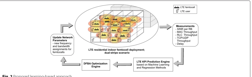
In a nutshell, our goal is to design a general framework for LTE network performance prediction and optimization, that is easy to deploy in a real LTE system and able to adapt to the actual network conditions during normal opera-tion. In Fig. 2, we illustrate our proposed approach. As shown in the figure, we focus mainly on LTE indoor small cell network deployments and, in terms of evaluation, on the typical LTE residential dual-stripe scenario described in [27]. This scenario characterizes not only interactions among neighboring small cells within the same building but also among small cells belonging to adjacent buildings. According to our approach, the measurements are gath-ered from both LTE users and LTE small cells. On the user side, we gather measurements related to the performance achieved by user, i.e., throughput, and delay, and the cor-responding measurements related to channel conditions, i.e., SINR per RB. On the small cells side, we gather radio link control (RLC) and MAC layer statistics, and various throughput performance measurements. These measure-ments are then used to calculate different metrics which are then used for network performance predictions by the

LTE KPI Prediction Engine. This engine is leveraging dif-ferent machine learning and regression methods to realize the LTE KPI prediction functionality. The predicted LTE KPI values are then forwarded to theDFBA Optimization Enginewhich is using these values together with network measurements to inspect how near the current network performance is to the estimated optimal performance for the currently measured network conditions. If the DFBA Optimization Engine estimates that the change in network configuration will compensate possible trade-offs (e.g., interruption in service), it schedules the reconfiguration of the frequency and bandwidth assignment.

Our approach follows the centralized SON (CSON) architecture, according to which there is a centralized node that oversees operation of all small cells and con-trols their behavior. In CSON architecture, the centralized node receives inputs from small cells and determines their configuration. Thus, theLTE KPI Prediction Engine

and the DFBA Optimization Engine are placed at the centralized node. Since the configuration parameters are not going to be changed frequently, the proposed solu-tion should not be affected by the latency due to the communication exchange between small cells and the cen-tralized node. Also, the network overhead is low, since the measurement information from the small cells to the central node can be scheduled per best-effort basis. Note that this architecture is compliant with the con-trol plane solution for MDT which is discussed in 3GPP TR32.827 [28]. Thus, the main message exchanges in our approach are between user equipments (UEs) and small cells and between small cells and the centralized manage-ment node, and all the interfaces needed for implemanage-menting our solution are already present in the standard.

The main contribution of the proposed approach is the learning-based LTE KPI performance estimation. Even if in this work we apply this approach to the frequency and bandwidth assignment use case, we argue that this approach is much more general and may be used for a larger set of configuration parameters and for different utility-based network planning and optimization tasks [9], where the accurate prediction of KPIs are necessary for an effective optimization.

3.4 LTE KPI prediction engine

To realize the LTE KPI prediction engine, we propose a learning-based approach according to which different KPIs are accurately predicted by using regression anal-ysis and machine learning techniques based on basic pathloss and configuration information combined with a limited number of feedback measurements that pro-vide the throughput and the delay metrics for a partic-ular frequency and bandwidth setting. As discussed in Section 3.2, we aim at designing a solution that requires a minimal amount of training for active exploration. More-over, the prediction engine should be able to predict dif-ferent KPIs, e.g., the network-wide and per-user LTE KPIs. To achieve all these requirements and to select the best candidate for the prediction engine, we study and compare the performance of various classical and modern predic-tion techniques. We list and explain these techniques in Section 3.5.

These prediction techniques leverage various param-eters, metrics, and derived inputs. The latter are usu-ally called covariates or regressors in the statistical and machine learning literature. Among the covariates being used in this paper, the most are being calculated by using

the SINR/MAC throughput mapping. This mapping rep-resents the network MAC layer throughput calculation based on the actual network measurements. We calculate this mapping in the following way. According to the LTE standard, UEs are periodically reporting to the base sta-tion a channel quality indicator (CQI) per each subband and wideband. We use this value at the MAC layer of the base station for AMC mapping, i.e., to determine the size of the transport block (TB) to be transmitted to the UE. A typical AMC behavior is to select a TB size that yields a BLER between 0 and 10 % [29]; the TB size for each given modulation and coding scheme and number of RBs are given by the LTE specification in [30].

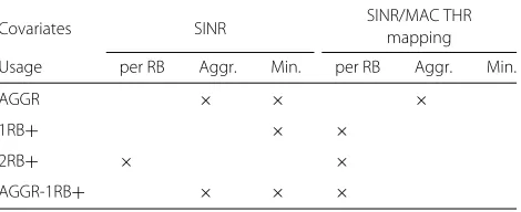
Moreover, we investigate the performance for differ-ent combinations of covariates. Since the covariates can be combined on a per-RB basis or aggregated together in various ways (such as considering the minimum or the sum of SINRs over the band), the number of dif-ferent combinations of covariates is very large. Here, we limit our attention to a small number of representative combinations summarized in Table 1.

Additionally, we consider the effect on prediction per-formance of different sampling methods, i.e., random

and stratified sampling. In statistics,stratified sampling

is obtained by taking samples from each stratum or sub-group of a population, i.e., a mini-reproduction of the population is achieved; conversely, according the ran-dom samplingmethod, each sample is chosen entirely by chance in order to reduce the likelihood of bias. While

stratified sampling requires more effort for data prepa-ration, it is appealing for its higher prediction accuracy in scenarios where the performance varies among differ-ent sub-groups of population or sampling regions. For the stratified sampling method, we define the sampling regions by calculating the aggregated network throughput based on the SINR/MAC throughput mapping previously described.

Finally, we analyze performance prediction by means of goodness of fit metrics, such as the prediction error in network-wide and per-user throughput estimation, evalu-ating how they depend on the size of the training set. This allows us to determine the ability of the proposed solution to learn during real-world operation.

Table 1Considered combinations of covariates

Covariates SINR SINR/MAC THR_mapping

Usage per RB Aggr. Min. per RB Aggr. Min.

AGGR × × ×

1RB+ × ×

2RB+ × ×

3.5 Statistical and machine learning methods for LTE KPI prediction engine

In this section, we provide an overview of the different sta-tistical and machine learning methods being studied for the realization of the LTE KPI prediction engine. We begin with a basic overview of the principles and terminology involved, and then give a concise summary on the princi-ples of the methods used. For further information on the prediction techniques being used, the interested reader is referred to [31] and [32].

The objective of all of the methods considered, regard-less of whether statistical or machine learning based, is to find a function thatpredictsthe value of a dependent variabley=f(x1,. . .,xn)as a function of various

predic-torsorcovariates xi. Usually, this is done by conducting

a limited number of experiments that yield the value ofy

for known values of the covariates that are then used to

fitortrainthe model. The functional form of the model as well as the training procedure used are the main dif-ferences between the different methods. In our case, the

ycorresponds to a performance metric of interest, and the differentxi are measurements of network conditions

(signal-to-interference-plus-noise ratio (SINR) values for different nodes) as well as available prior data (such as theoretical MAC layer throughput at given SINR).

The simplest method used for establishing a baseline prediction performance is LM that simply modelsyas a linear function of the covariates, as in

y=a0+

iaixi. (2)

The coefficientsai are determined based on the training

data for example by minimizing the root mean squared error (RMSE) of the predictor. Linear regression also has in our context a simple communication-theoretic interpretation: in the high SINR regime, linear functions approximate well the Shannon capacity formula, and y

becomes simply the best approximation of the network throughput as a optimal weighted sum of the individ-ual Shannon capacity estimates. Thus, linear regression can be used as an improved proxy for simple Shannonian SINR-based network capacity models. Simple generaliza-tion of this basic scheme is to apply a transformageneraliza-tion function to each of the termsaixi. The generalized

regres-sion techniques thus obtained are usually calledprojection pursuit regression(PPR) methods.

The simplest non-traditional prediction method we consider is theKnearest neighbors algorithm (KNN for short). For KNN, we consider the covariatesxi as

defin-ing a point in an Euclidean space, with the value of theyobtained from the corresponding experiment being assigned to that point. When predictingyforx_ifor which experimental data is not available, we find theK near-est neighbors of the pointx_i from the training data set in terms of the Euclidean distance. Our prediction is

then the distance-weighted average of the correspond-ing values of y. The KNN algorithm is an example of a non-parametric method that requires no estimation pro-cedure. This makes it easy to apply, but limits both its abil-ity to generalize beyond the training data and the amount of smoothing it can perform to counter the effects of noise and other sources of randomness on the predictions.

A much more general and powerful family of regression techniques is obtained by considering trees of individ-ual regression models. The model corresponds to a tree graph, with each non-leaf vertex corresponding to choos-ing a subspace by imposchoos-ing an inequality of some of the

xi. The leaves of the tree finally yield the predictions y

as the function of the ancestor vertices partitioning the space ofxiinto subsequently finer subspaces. The various

regression tree algorithms proposed in the literature dif-fer mainly in the method used to choose the partitioning in terms of the covariatesxi, as well as in the way

train-ing data is used to find the optimum selection of decision variables in terms of the chosen partitioning scheme. We consider bothboosting(boosted tree (BTR)) andbagging

(TBAG) in the process of finding optimal regression tree. Of these, bagging usesbootstrap(sampling with replace-ment to obtain large number of training data sets from a single one) with different sample sizes to improve the accuracy of the parameter estimates involved. Boosting on the other hand performs retraining of the model sev-eral times, with each iteration giving an increased weight to samples for which the previous iterations yielded poor performance result. The final prediction from a boosted tree is a weighted average of the predictions from the individual iterations. In general, regression trees are a very powerful and general family of prediction methods that should be considered as a potential solution to any non-trivial prediction or learning problem.

original input space defined by the xi, this is often

pos-sible in the high-dimensional feature space obtained by mapping the covariates with thekernel function. In the fol-lowing, we use SVMs with basic radial basis functions for regression.

The last family of machine learning techniques we con-sider in our study is that of self-organizing maps also known asKohonen networks (KOH). These form a fam-ily of artificial neural networks, for which eachneuron(a vertex on a lattice graph) carries a vector of covariates ini-tialized to random values. The training phase iterates over the training data set, finds the nearest neighbor to each vector of covariates from this set and the neural network, and updates the corresponding neuron and its neighbors to have higher degree of similarity with the training vector. Over time, different areas of the neural network converge to correspond to different common types occurring often in the training data set. While originally developed for classification problems, the Kohonen network can be used for regression by assigning a prediction function (such as the simple linear regression) to each class discovered by the neural network.

The considered KPIs, prediction methods and metrics, regressors, and sampling methods are summarized in Table 2. We use the R environment, and in particular the caret package, as the basis of our computations [32].

4 Performance evaluation

4.1 Evaluation setup

We consider a typical LTE urban dual stripe building sce-nario defined in [27] and the corresponding simulation assumptions and parameters defined in [33]. In Fig. 3, we show a radio environmental map of one instance of the simulated scenario. Each building has one floor which has eight apartments. The small cells (home eNodeBs) and users are randomly distributed in the buildings. Each home eNodeB has an equal number of associated UEs and

Table 2Considered KPIs, prediction methods and metrics, regressors and sampling methods

KPIs Network throughput; user throughput

Prediction methods Bagging tree (TBAG, Treebag)

Boosted tree (BTR)

Kohonen network (KOH)

SVM radial (SVM)

K-nearest neighbor (KNN)

Projection pursuit regression (PPR)

Linear (LM)

Prediction metrics RMSE user fit; 95th percentile RMSE

Regressors SINR; SINR/MAC throughput mapping

Sampling Random; stratified

Fig. 3Radio environmental map of dual-stripe scenario with one block of two buildings. Each home eNodeB has connected three UEs that are located in the same apartment

is placed in a separate apartment along with its associated UEs. By using the random distribution, we aim at simulat-ing the scenario that corresponds to the greatest extent to a realistic residential small cell deployment. The random placement of small cells in each independent simulation along with the random placement of the users adds to the simulation additional degree of randomness, which is con-sequently increasing the credibility of obtained simulation results. We concentrate on studying the following network configurations:

• 4 home eNodeBs, 12 users, and a total system bandwidth of 2 MHz

• 4 home eNodeBs, 8 users, and a total system bandwidth of 5 MHz

• 2 home eNodeBs, 20 users, and a total system bandwidth of 2 MHz

applications, we neglect the first interval of 5 s of each simulation execution. We configure simulations by using different combinations ofBandfc, and we configure other

network parameters according to Table 3. Different ran-dom placements of small cells and users are achieved by running each simulation configuration with different values of the seed of the random number generator.

To simulate the scenarios, we use the ns-3-based LTE-EPC network simulator (LENA) [35] which features an almost complete implementation of the LTE protocol stack, from layer two above, together with an accurate simulation model for the LTE physical layer [29]. The use of such detailed simulator provides a performance evalu-ation which is reasonably close to that of an experimental LTE platform.

4.2 Results on the correlation between covariates and KPIs

We begin by illustrating the challenges of MAC layer throughput prediction based on a SINR metric. For this

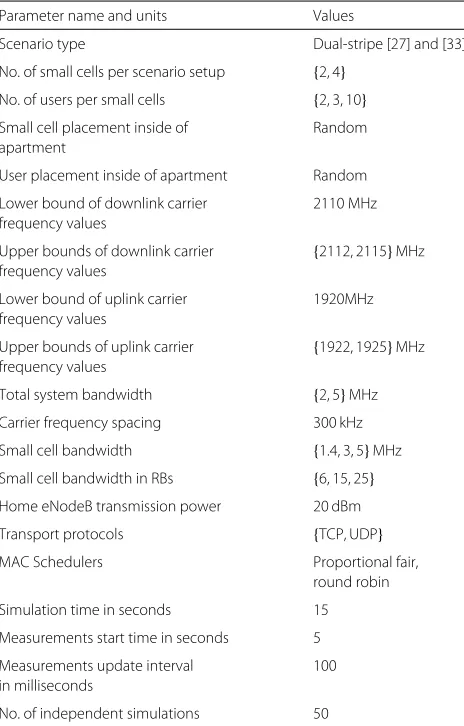
Table 3Evaluation configuration parameters

Parameter name and units Values

Scenario type Dual-stripe [27] and [33]

No. of small cells per scenario setup _{2, 4_}

No. of users per small cells _{2, 3, 10_}

Small cell placement inside of Random apartment

User placement inside of apartment Random

Lower bound of downlink carrier 2110 MHz frequency values

Upper bounds of downlink carrier {2112, 2115}MHz frequency values

Lower bound of uplink carrier 1920MHz frequency values

Upper bounds of uplink carrier {1922, 1925}MHz frequency values

Total system bandwidth {2, 5}MHz

Carrier frequency spacing 300 kHz

Small cell bandwidth _{1.4, 3, 5_}MHz

Small cell bandwidth in RBs _{6, 15, 25_}

Home eNodeB transmission power 20 dBm

Transport protocols {TCP, UDP}

MAC Schedulers Proportional fair, round robin

Simulation time in seconds 15

Measurements start time in seconds 5

Measurements update interval 100 in milliseconds

No. of independent simulations 50

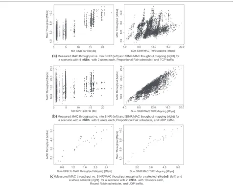
analysis, we select the Sum SINR, Sum/THR Mapping, andMin SINR per RBcovariates that were introduced in Section 3.4. TheSum SINRcovariate is calculated as the raw sum of SINRs per RB. TheSUM/THR Mapping repre-sents the MAC layer throughput calculated as a function of the raw sum of SINRs per RB according to the through-put calculation based on the the AMC scheme, which is explained in Section 3.4. The Min SINR per RB covari-ate is the minimum SINR perceived per RB. The SINR metric is calculated by leveraging on the pathloss mea-surements gathered at each UE. In Fig. 4, we show the actual measured system-level MAC layer throughput as a function of eitherSum SINRorSum/THR Mappingbased on 337 simulation results. Points in the figures correspond to measurements obtained from different simulation executions.

Fig. 4Actual measured performance vs. pathloss-based SINR and 3GPP based mapping of these values to MAC throughput. System bandwidth of 2 MHz, 4 small cells with 3 associated users each

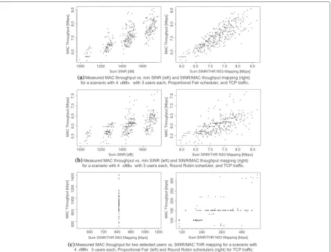
the following, we consider the correlation ofMin SINR per RBandMAC Throughput.

In Fig. 5, we illustrate correlations between the KPI and the selected covariates on a much larger data set which contains 4625 samples. These samples are achieved by configuring a larger system bandwidth, 5 MHz, which allows for much larger number of frequency and band-width assignment combinations, as we explained in Section 3.2. As we show in the following discussion, the analysis on a larger data set confirms the trends that were observed for a smaller data sets in Fig. 4. In Fig. 5a, b, we note the strong correlation between the transport protocol type and the measured MAC layer throughput. When the transport protocol is UDP, there is a strong correlation between theMAC Throughput and theSum SINR/MAC THR Mapping covariate. On the other hand, when TCP is being used, there is a weak correlation, i.e., it is harder to predict the KPIs. This is an expected behavior because of the complex interplay between the

TCP congestion control and the LTE PHY, MAC, and RLC layers. We also note from these two figures that there is no strong correlation between MAC Through-put and Min SINR per RB, so that the dispersion of results for the round robin scheduler shown in Fig. 4c is not caused by assigning the min SINR per RB to UEs. Figure 5c shows that the correlation remains strong when eNodeBs are configured to use the round robin sched-uler instead of proportional fair and that the Sum SINR

and the Sum SINR/MAC THR Mapping covariates can be used almost interchangeably for predictions. We also note that the smaller number of users increases the dis-persion in the SINR vs. MAC throughput dependency even further.

Fig. 5Actual measured performance vs. pathloss-based SINR, and 3GPP-based mapping of these values to MAC throughput. System bandwidth of 5 MHz. Setup with four small cells each having associated two users inaandb; two small cells each having associated ten users inc

while predicting both system-level and user-level KPIs, is a challenging problem.

4.3 Performance of prediction methods

Following the conclusions derived in Section 4.2, we select the scenario setup and regressors for the performance comparison of the LTE KPI prediction methods. Namely, we select the configuration that appears the most com-plex for prediction, i.e., the configuration manifested by low or lack of linear correlation between the predicted KPI and covariates, that is the network configuration in which small cells operate with the proportional fair MAC sched-uler and UEs traffic goes over TCP. Additionally, based on a study from Section 4.2, we select the aggregate regres-sors, since they appear to have a higher correlation with KPI thanMin SINR per RB. The total of 4625 samples are obtained by running the small cell network scenario that consists of four small cells with two users associated to

each of them, while the total system bandwidth is 5 MHz. The training data for each prediction method is obtained by selecting 10 % of samples by random sampling method. The testing data samples are generated based on measure-ments for each user in the scenario, with a total of 50 inde-pendent samplings and regression fittings samples. We consider the following prediction techniques: bagging tree (TBAG), BTR, KOH, SVM radial (SVM), K-nearest neigh-bor (KNN), PPR, and linear regression method (LM), all of which we explained in detail in Section 3.5. Finally, in Fig. 6, we show the results of the prediction performance of different prediction methods. For boxplots, the three lines of the box denote the median together with the 25th and 75th percentile, while the whiskers extend to the data point at most 1.5 interquartile ranges from the edge of the box.

Fig. 6Comparison of prediction methods over random sampling of 10 %

the simplest prediction method, LM, has the highest RMSE and consequently the poorest prediction perfor-mance ratio. The poor perforperfor-mance of the LM method indicates that analytical models based on Shannonian capacity estimates are also expected to perform poorly. Note also that the gain of more advanced methods over LM lower bounds the gain compared to even simpler schemes, such as full frequency reuse or orthogonalized channelization. More advanced prediction techniques based on regression, PPR and KNN, are computationally extremely fast ( 1ms for the tested sample set), which can thus be useful to offer an intermediate solution in sit-uations in which more computationally expensive meth-ods are not feasible. Among advanced machine learning techniques, SVMs and KOH networks perform the poor-est, and the latter technique shows additionally a large variability in the performance prediction accuracy. Both tree-based methods (TBAG and BTR) perform consis-tently better than all previous methods in terms of raw performance and variability of results; finally, the TBAG method achieves the best prediction performance. This superior performance is expected due to the very nature of TBAG and BTR. Use of bootstrap samples results in both of these methods being essentially not an individ-ual machine learning optimizer, but anensemble learner

conducting voting between large number of individual models. Such combinations of models usually outperform

individual ones by wide margin at the cost of larger storage and training overhead [31]. Based on the latter discussion, we conclude that TBAG is the most promising method for the prediction engine.

4.3.1 Prediction performance validation for different sizes of the training set

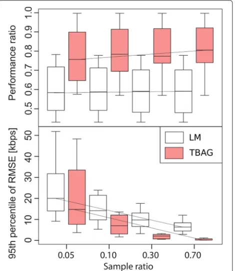
In the following, we evaluate the prediction performance of TBAG as a function of the size of the training set, i.e., in order to assess how fast it can learn when deployed in an actual scenario. We carry out a performance eval-uation study using the same small cell network scenario setup that we used for the comparison of the predic-tion techniques. We compare TBAG with the LM method in order to analyze the advantage of the application of advanced prediction techniques instead of simple predic-tion techniques for different sizes of the training set. For this performance evaluation, we define the performance ratio metric as the ratio of the network throughput of the frequency and bandwidth allocation chosen by solv-ing the optimization problem with the considered model to the network throughput of the best possible frequency and bandwidth configuration, i.e., the one that would be allocated by an exhaustive search algorithm. The pur-pose of this metric is to give a measure of how close a given solution is to the optimal frequency and band-width assignment. In Fig. 7, we show the results of the

prediction performance for different sizes of the training set. The black lines in the figures show the tendencies in the plot, while the boxplots are generated in the same way as for the results shown in Fig. 6. By observing the RMSE from Fig. 7, we note that for more accurate perfor-mance more samples need to be taken, though this does not necessarily translate into a better network optimiza-tion performance, which is the case for the LM method. Additionally, we conclude that the benefit of advanced prediction techniques over simpler prediction techniques is not only the ability to learn on a very small sample set but is also the ability to improve its performance over time. Both characteristics are crucial for a real net-work deployment, as we seek a solution that can net-work good with minimum a priori knowledge, and that is able to improve performance by exploiting real-time network measurements.

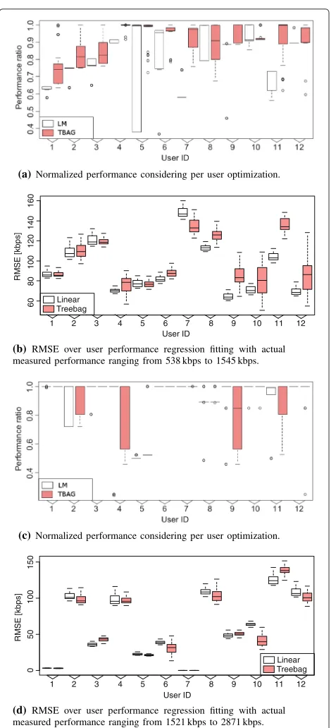
4.3.2 Prediction performance validation for different LTE KPIs and network configurations

We continue the TBAG performance analysis by test-ing the prediction of different KPIs metric under various network configurations. Specifically, whereas before we evaluated TBAG in the context of optimizing system level KPI, we now focus on the performance prediction of TBAG in terms of user-level KPIs. We evaluate the per-formance obtained with differently configured small cell network setups. The fixed scenario parameters are the sys-tem bandwidth is 2 MHz, network has 4 small cells, and a total of 12 users. We run independent batch simula-tions that have in common the small cell network topol-ogy, but differently configured transport protocols used by UEs’ applications (TCP or UDP) and different MAC scheduler (proportional fair or round robin). Out of the four combinations (two different schedulers, two different transport protocol types) that we evaluated, we illustrate the performance of TBAG vs. LM in Fig. 8 for the two most interesting cases: (1) eNodeBs employing the pro-portional fair scheduler and UEs traffic going over TCP and (2) eNodeBs employing the round robin scheduler and UEs traffic over UDP. Our results confirm that the TBAG method performs well for different scenario setups. Here, the TBAG method outperforms the LM method, especially in the case of TCP and the proportional fair scheduler (Fig. 8a, b). We note that the results shown in Fig. 6 also hold on a per-user basis, as well as in more complex and dynamic network scenario (TCP and pro-portional fair scheduler being used). Figure 8c, d shows a similar collection of results, but for the case of UDP with the round robin scheduler. Here, even the simple LM method performs nearly optimal due to the simplified higher-layer interactions explained in Section 4.2. These figures confirm the previously formulated hypothesis that the network configuration with the simpler setup (UDP

(a)Normalized performance considering per user optimization.

60

(b) RMSE over user performance regression fitting with actual measured performance ranging from 538 kbps to 1545 kbps.

(c)Normalized performance considering per user optimization.

1 2 3 4 5 6 7 8 9 10 11 12

(d) RMSE over user performance regression fitting with actual measured performance ranging from 1521 kbps to 2871 kbps.

and more simple scheduler, such as round robin) results in a higher predictability.

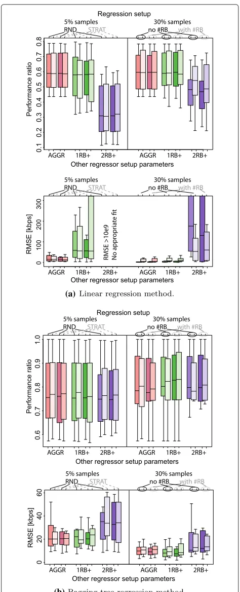
4.3.3 Prediction performance validation for different covariates and sampling methods

We evaluate the performance of the TBAG prediction method for different covariates and different sampling methods: the random and the stratified sampling, all of which were explained in Section 3.4. Figure 9 summaries the performance of the TBAG method and the LM with different covariates being used, together with two sam-pling methods over 5 and 30 % samples being taken. The stratified sampling results in better performance than the simple random selection of the configurations used to train the predictor. The basic AGGR covariate is out-performed by the 1RB+ regressor if complex machine learning-based methods are applied, as those can make use of the additional information available through them (see Table 1 for the covariate abbreviations). For LM, due to the non-linear nature of this additional information, the performance impact is actually negative. In general, only advanced machine learning and regression techniques are able to benefit from more complex covariates, such as per-RB measurements, provided that a large enough sampling base is available (which was not the case for the 2RB+ regressor).

4.4 Performance evaluation of proposed learning-based DFBA approach

Finally, in this section, we present the major results of this work by evaluating the network performance achieved for DFBA when the proposed learning-based approach is used and comparing it with the case where prediction methods based on pathloss-based mathematical models that use SINR and MAC throughput mapping estimates (sum or minimum of those over the RBs) are used. The performance gain is expressed as the percentage of the maximum achievable network performance obtained by applying an exhaustive search method to solve the DFBA problem. The learning-based DFBA approach is using the TBAG method for LTE KPI predictions which is trained by using the stratified sampling method and is employing the active probing in addition to pathloss values. Table 4 shows the performance obtained when using different prediction methods for solving the frequency and band-width optimization problem explained in Section 3.2 with the goal of total network throughput maximization.

The scenario label identifies the number of small cells/number of users, the percentage of samples taken, and the employed transport layer and schedulers. The gains obtained by using the learning based DFBA range between 6 and 43 %. We note that the gain is largest for

(a)

(b)

Table 4Comparison of DFBA performance when different prediction approaches are used

Scenario conf. and sample set size 4/12, 2 MHz, 10 % 4/8, 5 MHz, 5 %

Transport protocol TCP UDP TCP UDP

MAC scheduler PF RR PF RR PF RR PF RR

SINR 85 % 83 % 83 % 86 % 53 % 54 % 53 % 42 %

Min SINR 91 % 82 % 89 % 89 % 71 % 77 % 58 % 49 %

Sum SINR/MAC THR Mapping 72 % 72 % 70 % 81 % 61 % 61 % 35 % 43 %

Min SINR/MAC THR Mapping 89 % 81 % 88 % 89 % 55 % 64 % 55 % 50 %

Learning based (TBAG) 100 % 85 % 100 % 95 % 96 % 95 % 97 % 92 %

Exhaustive search 100 % 100 % 100 % 100 % 100 % 100 % 100 % 100 %

Exhaustive search (Mbps) 9 8 9 7 12 10 26 25

the more complex scenarios, which means that even larger gains are expected for more complicated performance optimization goals, e.g., ones that include a fairness met-ric. Overall, the results provided in Table 4 show that the learning-based DFBA approach results in the selection of a network configuration that performs better compared to the SINR-based models and is close-to-optimal.

5 Conclusions

In this paper, we investigated the problem of perfor-mance prediction in LTE small cells and we studied its application to dynamic frequency and bandwidth assign-ment in an LTE small cells network scenario. We proposed a learning-based approach for LTE KPI per-formance prediction, and we evaluated it by using data obtained from realistic urban small cell network simu-lations. The results firmly show that the learning-based performance prediction approach can yield very high per-formance gains. The outstanding aspect of the learning-based DFBA approach is that the high performance gains are obtained for a reasonably small number of measure-ments, which allows for its implementation in a real LTE system. Among the studied prediction methods, the bagging tree prediction method results to be the most promising approach for LTE KPI predictions compared to other techniques, such as boosted trees, Kohonen net-works, SVMs, K-nearest neighbors, projection pursuit regression, and linear regression methods. Another con-clusion of the comparative study on the prediction meth-ods for the LTE network performance prediction is that the used performance metric and RMSE should be consid-ered together when evaluating the different performance prediction methods. In particular, a high RMSE does not always lead to poor optimization results, and, if maxi-mum performance grows, RMSE may also increase due to higher variance, but the main tendency of prediction might not change. Finally, we show that the DFBA based on LTE KPI prediction achieves in average performance improvements of 33 % over approaches involving simpler

SINR-based models. Moreover, the learning-based DFBA performs very close to optimal configuration, achieving on average 95 % of the optimal network performance.

Acknowledgements

The work done at CTTC was made possible by grant TEC2014-60491-R (Project5GNORM) by the Spanish Ministry of Economy and Competitiveness. The work done at RWTH was partially funded by the FP7-ICT ACROPOLIS project.

Competing interests

The authors declare that they have no competing interests.

Author details

1_{Centre Tecnològic de Telecomunicacions de Catalunya (CTTC), 08860}

Castelldefels, Av. Carl Friedrich Gauss 7, Spain.2_{Institute for Networked}

Systems at RWTH Aachen University, 52072 Aachen, Kackert Street, Germany.

Received: 4 February 2016 Accepted: 27 July 2016

References

1. NGMN Technical Working Group Self Organising Networks, Next generation mobile networks use cases related to self organising network, Overall Description (2008)

2. ETSI, 3GPP TR 36.902, LTE; E-UTRAN; Self-configuring and self-optimizing network (SON) use cases and solutions (Release 9) (2011)

3. Cisco Service Provider Wi-Fi, A platform for business innovation and revenue generation. http://www.cisco.com, 2012. Accessed December 2015

4. J Weitzen, L Mingzhe, E Anderland, V Eyuboglu, Large-scale deployment of residential small cells. Proc. IEEE.101(11), 2367–2380 (2013). doi:10.1109/JPROC.2013.2274325

5. T Zahir, K Arshad, A Nakata, K Moessner, Interference management in femtocells. IEEE Commun. Surv. Tutor.15(1), 293–311 (2011). doi:10.1109/SURV.2012.020212.00101

6. S Hamalainen, H Sanneck, C Sartori (eds.),LTE self-organising networks

(SON): network management automation for operational ffficiency(Wiley,

2011). doi:10.1002/9781119961789

7. J Mitola III, GQ Maguire, Cognitive radio: making software radios more personal. IEEE Pers. Commun.6(4), 13–18 (1999). doi:10.1109/98.788210 8. RW Thomas, LA DaSilva, AB MacKenzie, Cognitive networks. Proceedings

of IEEE DySPAN (2005). doi:10.1109/DYSPAN.2005.542652

9. M Bkassiny, Y Li, S Jayaweera, A survey on machine-learning techniques in cognitive radios. IEEE Commun. Surv. Tutor.15(3), 1136–1159 (2013). doi:10.1109/SURV.2012.100412.00017

11. Stoke, Zhilabs, Analytics in secured LTE. http://www.zhilabs.com/new_z/ wp-content/uploads/2014/06/150-0045-002_SB_Stoke_Zhilabs_ AnalyticsSecuredLTE_Final1.pdf, Accessed Deccember 2015 12. Samsung, Smart LTE for future innovation. http://www.samsung.com/

global/business/networks/smart-lte, Accessed December 2015 13. N Baldo, L Giupponi, J Mangues-Bafalluy, inProceedings of European

Wireless. Big data empowered self organized networks, (2014)

14. S Sesia, I Toufik, M Baker,LTE—the UMTS long-term evolution (from theory

to practice). (John Wiley and Sons Ltd, 2009). doi:10.1002/9780470742891

15. E Dahlman, S Parkvall, J Skold,4G: LTE/LTE-Advanced for mobile broadband. (Academic Press (Elsevier), 2013). doi:10.1016/B978-0-12-419985-9. 01001-1

16. W Hale, Frequency assignment: theory and applications. Proc. IEEE. 68(12), 1497–1514 (1980). doi:10.1109/PROC.1980.11899 17. H Zhuang, et al., Dynamic spectrum management for intercell

interference coordination in LTE networks based on traffic patterns. IEEE Trans. Vehic. Technol.62(5), 1924–1934 (2013). doi:10.1109/TVT.2013. 2258051

18. Z Lu, T Bansal, P Sinha, Achieving user-level fairness in open-access femtocell-based architecture. IEEE Trans. Mobile Comput.12(10), 1943–1954 (2013). doi:10.1109/TMC.2012.157

19. L Tan, et al., inProceedings of IEEE WCNC. Graph coloring based spectrum allocation for femtocell downlink interference mitigation, (2011). doi:10.1109/WCNC.2011.5779338

20. S Sadr, R Adve, inProceedings of IEEE ICC. Hierarchical resource allocation in femtocell networks using graph algorithms, (2012).

doi:10.1109/ICC.2012.6364427

21. S Uygungelen, G Auer, Z Bharucha, inProceedings of IEEE VTC. Graph-based dynamic frequency reuse in femtocell networks, (2011). doi:10.1109/VETECS.2011.5956438

22. YL Lee, TC Chuah, J Loo, Recent advances in radio resource management for heterogeneous LTE/LTE-A networks. IEEE Commun. Surv. Tutor.16(4), 2142–2180 (2014). doi:10.1109/COMST.2014.2326303

23. FF Bernardo, RR Agusti, JJ Perez-Romero, O Sallent, Intercell interference management in OFDMA networks: a decentralized approach based on reinforcement learning. IEEE Trans. Syst. Man Cybernetics, Part C: Appl. Rev.41(6), 968–976 (2011). doi:10.1109/TSMCC.2010.2099654

24. ETSI, 3GPP TS 36.104, LTE; E-UTRA; Base station (BS) radio transmission and reception (Release 12) (2015)

25. ETSI, 3GPP TS 36.106, LTE; E-UTRA; FDD repeater radio transmission and reception (Release 12) (2014)

26. A Imran, A Zoha, Challenges in 5G: how to empower SON with big data for enabling 5G. IEEE Netw.28(6), 27–33 (2014).

doi:10.1109/MNET.2014.6963801

27. ETSI, 3GPP TS 36.814; Technical specification group radio access network; E-UTRA; Further advancements for E-UTRA physical layer aspects (Release 9) (2010)

28. 3GPP TS 32.827, Technical Specification Group Services and System Aspects; Telecomunication management; Integration of device management information with Itf-N (Release 10) (2010)

29. M Mezzavilla, M Miozzo, N Baldo, M Zorzi, inProceedings of ACM MSWiM. A lightweight and accurate link abstraction model for the simulation of LTE networks in ns-3, (2012). doi:10.1145/2387238.2387250

30. ETSI, 3GPP TS 36.213, LTE; E-UTRA; Physical layer procedures (Release 12) (2014)

31. T Hastie, R Tibshirani, JJH Friedman,The elements of statistical learning. (Springer New York, 2001). doi:10.1007/978-0-387-84858-7

32. M Kuhn, Building predictive models in R using the caret package. J. Stat. Softw.28(5), 1–26 (2008)

33. ETSI, 3GPP TS 36.828, Technical Specification Group Radio Access Network; E-UTRA; Further enhancements to LTE Time Division Duplex (TDD) for Downlink-Uplink (DL-UL) interference management and traffic adaptation (Release 11) (2012)

34. F Capozzi, G Piro, LA Grieco, G Boggia, P Camarda, Downlink packet scheduling in LTE cellular networks: key design issues and a survey. IEEE Commun. Surv. Tutor.2(15), 678–700 (2013). doi:10.1109/SURV.2012. 060912.00100

35. N Baldo, M Miozzo, M Requena-Esteso, J Nin-Guerrero, inProceedings of

ACM MSWiM. An open source product-oriented LTE network simulator

based on ns-3, (2011). doi:10.1145/2068897.2068948

Submit your manuscript to a

journal and benefi t from:

7Convenient online submission 7Rigorous peer review

7Immediate publication on acceptance 7Open access: articles freely available online 7High visibility within the fi eld

7Retaining the copyright to your article