R E S E A R C H
Open Access
The intervals of oscillations in the
solutions of the Legendre differential
equations
Dimitris M Christodoulou
1, James Graham-Eagle
1and Qutaibeh D Katatbeh
2**Correspondence: available at the end of the article
Abstract
We have previously formulated a program for deducing the intervals of oscillations in the solutions of ordinary second-order linear homogeneous differential equations. In this work, we demonstrate how the oscillation-detection program can be carried out around the regular singular pointsx=±1 of the Legendre differential equations. The solutionsyn(x) of the Legendre equation are predicted to be oscillatory in|x|< 1 for
n≥3 and nonoscillatory outside of that interval for all values ofn. In contrast, the solutionsym
n(x) of the associated Legendre equation are predicted to be oscillatory for
n≥3 andm≤n– 2 only in smaller subintervals|x|<x∗< 1, the sizes of which are determined bynandm. Numerical integrations confirm that such subintervals are distinctly smaller than (–1, +1).
MSC: 34A25; 34A30; 42C05
Keywords: oscillations; second-order linear differential equations; analytical theory; transformations; Legendre differential equations
1 Introduction
It is well known (e.g., [], Section .; [], Section XI.) that all ordinary second-order linear homogeneous differential equations can be written in the general form
y+b(x)y+c(x)y= , ()
and that this form can be transformed to the canonical form
u+q(x)u= , ()
where the primes denote derivatives with respect to the independent variable x, q= –(b+ b– c)/, andy(x) =u(x)exp(–b(x)dx). The canonical form () condenses all the information regarding the coefficients of equation () intoq(x) and ‘oscillation theory’ focuses on this coefficient in order to derive the oscillatory properties of the solutions of equation () (see the reviews in [, ] and references therein). In a previous paper ([], here-after CGK), we also focused on theq(x) of equation (). We formulated a new definition of oscillation as the appearance of successive critical points of the same kind (maxima, or
minima, or inflection points) in the graph of a solution. Then we described a program for deducing the precise intervals of oscillations in the solutions of the general form (), and we presented a variety of examples in which this procedure was successful in predicting oscillatory behavior by examining the coefficientq(x) alone.
Some of the differential equations that were investigated by CGK were transformed to the harmonic-oscillator form with constant coefficients in the first step of the program, and their oscillatory properties were then derived easily from the discriminant of their characteristic quadratic equations. The rest of the equations were transformed to a form with constant damping (a constant coefficient of the first-derivative term), a quantity that clearly opposes any oscillatory tendencies in the solutions. In this second step of the pro-gram, a generalized Euler transformation of the independent variablexwas used:
x=c+cexp(kt), ()
wherec,c, andkare arbitrary constants, and a criterion for the intervals of oscillations
in the solutions was established:
q(x) > (x–c)
. ()
Only the constantcappears in the criterion and corresponds to a ‘horizontal shift’ of the
independent variablexin equation ().
The equations studied by CGK in the second step of the program contained singularities atx= or no singularities at all, in which casescwas set to zero in equations () and ().
In the present work, we extend our investigation to the study of oscillatory properties of the Legendre and associated Legendre equations [, ] that have regular singular points at x=± (that is, away fromx= ). In these cases, a horizontal shift c= proves to
be quite useful, since it can be chosen to circumvent one or the other singularity in the neighborhood of which the intervals of oscillations in the solutions are being sought. The other two constants in equation () are chosen in ways that allow for the investigation of specific intervals inx(in particular, ≤x< and <x<∞). We use the above equations in Section and Section below, where we analyze the Legendre equation and the associated Legendre equation, respectively. Finally, in Section , we summarize our results.
2 Legendre equation
wherenis a constant, is first transformed to the canonical form () in which the coefficient
q(x) is
q(x) =n(n+ )( –x
) +
( –x) , ()
andu(x) =y(x)| –x|. The coefficientq(x) is an even function ofx, so we can investigate
We choosec= andk= in equation (), in which case the transformation becomes
x= +cexp(t), ()
and the criterion () for oscillatory solutions becomes
q(x) >
(x– ). ()
By settingcto – or + in equation (), we can search for oscillatory solutions in intervals
on either side ofx= . Specifically, forc= –:
t∈(–∞, ] ⇒ x∈[, +),
and forc= +:
t∈(–∞, +∞) ⇒ x∈(+, +∞).
In both cases, equation () is the applicable criterion for oscillatory solutions, so these two intervals inxcan be investigated simultaneously. The pole atx= + is eliminated from the analysis when equations () and () are combined, in which case we find that the interval over which the solutions may oscillate is given by the solution of the algebraic inequality
Nx+ x– (N+ ) < ⇒ x∈(– – /N, +), ()
where
N≡(n+ ). ()
The endpointx–= – – /Nlies on the negative side of thex-axis, therefore oscillatory
solutions are predicted in the entire intervalx∈[, +). Furthermore, all solutions inx∈
(+, +∞) are predicted to be nonoscillatory.
Using the even symmetry of the canonical form () withq(x) given by equation (), we conclude that the solutions of the Legendre equation can oscillate only in the interval
|x|< . ()
On the other hand, we know from the results obtained by CGK that low-order polyno-mial solutions will be nonoscillatory and that the lowest-order solutions that may exhibit at least two critical points of the same kind (maxima, or minima, or inflection points) for certain choices of boundary conditions haven= . The borderline case withn= is discussed in the Nodal analysis below.
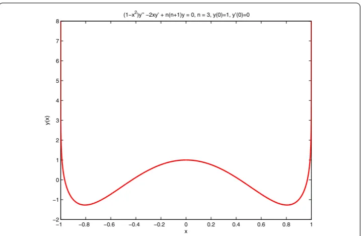
Figure 1 The numerical solution of equation (5) withn= 3 and boundary conditionsy(0) = 1 and
y(0) = 0.
Figure 2 The numerical solution of equation (5) withn= 4 and boundary conditionsy(0) = 0 and
y(0) = 1.
Nodal analysis. The above results can be better understood by counting the number of nodesN(n) inx∈[–, +] for the two types of boundary conditions used. Fory() = , the solutions are even and the number of nodes is
N(n) =
n, ifnis even,
while fory() = , the solutions are odd and then the number of nodes is
N(n) =
n+ , ifnis even,
n, ifnis odd, ()
where the node atx= has been counted for the odd solutions of equation (). Nodes at
x=± do not occur for anyn, not even in solutions that remain finite at these endpoints. The node counts clarify why the lowest-order oscillatory solutions occur forn= : the even solution hasN() = and develops two minima, so it is oscillatory. On the other hand, the odd solution has N() = and two extrema of the same kind do not occur, so it is nonoscillatory. Forn≥, both types of solutions have enough nodes to guarantee oscillatory behavior, and the number of nodes and oscillations increases with increasingn.
3 Associated Legendre equation
wherenandmare constants, is first transformed to the canonical form () in which the coefficientq(x) is
q(x) =n(n+ )( –x
) + ( –m)
( –x) , ()
andu(x) =y(x)| –x|. The coefficientq(x) is an even function ofx, so we can investigate
the intervalx≥ and the results will be applicable forx< as well.
We choose againc= andk= in equation (), in which case the transformation () is
applicable and the criterion for oscillatory solutions inx∈[, +∞) is given by inequality (). Substituting equation () into equation (), we find that the interval over which the solutions may oscillate is given by the solution of the algebraic inequality
Nx+ x– (N+ M) < ⇒ x∈(x–,x+), ()
Nis given by equation (), and
M≡ – m. ()
The endpointx–lies on the negative side of thex-axis, therefore oscillatory solutions are
predicted in the interval x∈[,x+). Furthermore, all solutions inx∈(x+, +∞) are
pre-dicted to be nonoscillatory.
interval|x|<x∗, where from equation ():
x∗≡x+=
N
– +√N+ MN+ . ()
It is easy to show thatx∗< for all values ofm= . Form= , thenM= and equation
() reduces tox∗= , as was also found in Section above for the Legendre equation.
Therefore, in all cases of interest (in whichm= and|m| ≤ |n|), the interval (–x∗, +x∗)
is a distinct subinterval of (–, +) and the oscillations of the solutions of the associated Legendre equation will have to cease before the solution curves approach the endpoints
x=±. Indeed, this behavior is observed in the numerical solutions of various cases with
m≥.
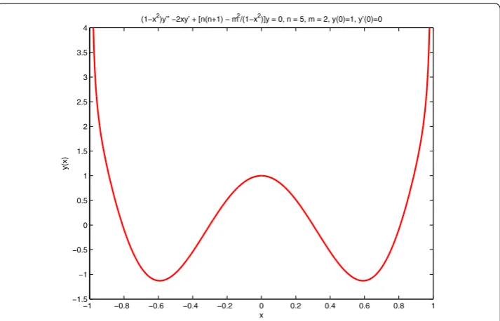
Numerical results. Figures and show two numerical solutions of equation () that oscillate in a distinct subinterval of (–, +). In Figure ,n= ,m= , and the boundary conditions arey() = andy() = . In Figure ,n= ,m= , and the boundary con-ditions arey() = andy() = . Additional numerical integrations show that, for larger values ofnand a fixed value ofm, the solutions exhibit increasingly more oscillations in (–x∗, +x∗) while the solutions outside of that interval are nonoscillatory for all values ofn.
Furthermore, for a fixed nand increasingm, the oscillation interval (–x∗, +x∗) shrinks
and the solutions exhibit progressively fewer nodes. Finally, form≥n– , some solutions do appear that are nonoscillatory over the entire interval (–, +). In the borderline case withm=n– , such nonoscillatory solutions depend critically on the adopted boundary conditions (see Figures and ), while form>n– , all solutions are nonoscillatory (see the Nodal analysis below). Two examples of the borderline case withm=n– = are shown in Figures and . The odd solution in Figure is nonoscillatory while the even solution in Figure exhibits two minima. Even in cases such as that of Figure , however,
Figure 4 The numerical solution of equation (14) withn= 12,m= 8, and boundary conditionsy(0) = 0 andy(0) = 1.The oscillations terminate atx∗≈ ±0.77, as predicted by equation (19).
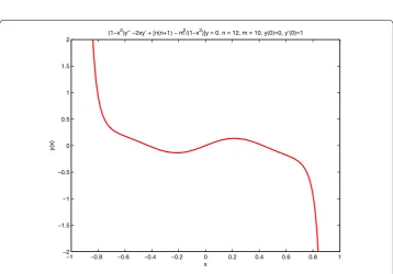
Figure 5 The numerical solution of equation (14) withn= 12,m=n– 2 = 10, and boundary conditions
y(0) = 0 andy(0) = 1.The solution is nonoscillatory as two extrema of the same kind do not appear in the interval (–0.60, +0.60) that is determined from equation (19).
the nonoscillatory solutions are distinctly nonmonotonic within the intervals specified by equation ().
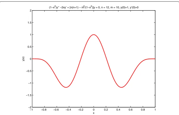
Figure 6 As in Figure 5 withm=n– 2 = 10, but for different boundary conditionsy(0) = 1 and
y(0) = 0.The solution is oscillatory in the interval (–0.60, +0.60), which is determined from equation (19).
the solutions are even and for ≤m≤n, the number of nodes is
N(n,m) =
n–m+ , ifn–mis even,
n–m+ , ifn–mis odd, ()
while fory() = , the solutions are odd and for ≤m≤n, the number of nodes then is
N(n,m) =
n–m+ , ifn–mis even,
n–m+ , ifn–mis odd, ()
where the node atx= has been counted for the odd solutions of equation (). The term + in both cases represents two nodes that occur atx=±. Form= , such nodes always occur for evenn–min even solutions (equation ()) and for oddn–min odd solutions (equation ()).
The node counts clarify the borderline case withm=n– . In this case,n–m= (even) and the even solutions all have nodes (equation ()), just enough for two extrema of the same kind to develop; so they are oscillatory. In contrast, the odd solutions have nodes (equation ()) and they are all nonoscillatory. Finally, form>n– , the solutions have a very small number of nodes (≤N(n,m)≤) and then oscillations cannot occur.
Alternative analysis of oscillations. The results shown in Figures - have been verified by an independent analysis inx∈(–, +) as follows: For|x|< , the substitution
x=sin(t), ()
transforms the associated Legendre equation () to the form
¨
where dots denote derivatives ofy(t) with respect tot. The canonical form () of this equation hasu(t) =y(t)√cos(t) and
q(t) =
N+ (M– )sec
(t), ()
whereNandMare given by equations () and (), respectively. Since these equations are strictly applicable in|t|<π/, then the criterion () for oscillatory solutions can be used withc= , in which case it reads
q(t) >
t. ()
Substituting equation () into equation (), we find that oscillatory solutions can occur in a subinterval of|t|<t∗<π/ in which
We have solved this inequality numerically for various values ofNandM, and the result-ing values ofx∗for all cases, including those depicted in Figures -, are virtually
identi-cal to those identi-calculated analytiidenti-cally from equation (). The agreement between results in the above two analyses justifies the use of a horizontal shift (c= ) in the former
analy-sis. Using horizontal shifts to remove singularities simplifies the calculations and leads to quadratic inequalities that can be solved analytically.
4 Summary
We have presented an analysis of the oscillatory properties of the solutions of the Legendre and associated Legendre differential equations [, ] that show two regular singular points in their coefficients away fromx= (atx=±). The analysis makes use of a program that was described in [] by CGK for investigating thex-intervals in which the solutions have an oscillatory character. According to this procedure, an attempt must first be made to transform a given equation to a form with constant coefficients. Unlike in the case of the Chebyshev equation that also has two poles atx=± but can be recast into a form with constant coefficients (CGK), the Legendre equations cannot be simplified in this manner and their analysis must proceed to the second step of the program, where a transformation ofx is applied in order to cast these equations into forms with constant damping (i.e., a constant coefficient of the first-derivative term). As was described in Sections and above, such a transformation is capable of eliminating from the analysis one or the other singularity, but not both of them at the same time. This leaves one pole in the coefficient of the canonical form of the final equation (equation () and equation ()) and its presence complicates the search for oscillatory solutions. Because the coefficients () and () of the canonical form are even functions ofx, it turns out that we can investigate only the interval
The results of our analysis are as follows:
(a) The solutionsyn(x)of the Legendre equation are predicted to be oscillatory in|x|< forn≥(according to the definition of oscillation given by CGK and adopted here as well) and nonoscillatory outside of that interval for all values ofn. Numerical integrations of many cases with a variety of boundary conditions confirm these predictions. Two examples of oscillatory solutions in(–, +)are shown in Figures and .
(b) The solutionsym
n(x)of the associated Legendre equation are predicted to be oscillatory forn≥only andm≤n– in smaller subintervals of|x|<x∗< , where x∗is given by equation (). (Note, however, that in the borderline case with m=n– , only the even solutions are oscillatory.) Numerical integrations, as well as a separate analysis of the alternative form () of the associated Legendre equation, confirm that such subintervals are predicted correctly and that they are distinctly smaller than the interval(–, +)of them= case. Three examples of oscillatory solutions are shown in Figures , , and and an example of a nonoscillatory solution is shown in Figure .
In the example of Figure withm=n– = , two extrema of the same kind do not occur in the predicted interval|x|< . because of the relatively large value ofm. In general, in the borderline case withm=n– , some solutions are oscillatory and other solutions are not, depending on the adopted boundary conditions (as in Figures and , respectively); but form>n– , all solutions are nonoscillatory because they exhibit just a small number of nodes ( to ). Even these types of solutions are, however, characteristically nonmono-tonic as they attempt to oscillate, but the small number of nodes does not permit a full ‘cycle’ to develop in the intervals|x|<x∗withx∗specified by equation ().
Competing interests
The authors declare that they have no competing interests.
Authors’ contributions
All authors drafted the manuscript, and they read and approved the submitted version.
Author details
1Department of Mathematical Sciences, University of Massachusetts Lowell, Lowell, MA 01854, USA.2Department of
Mathematics and Statistics, Jordan University of Science and Technology, Irbid, 22110, Jordan.
Acknowledgements
During this research project, DMC and JG-E were supported by the University of Massachusetts Lowell while QDK was on a sabbatical visit and was fully supported by the Jordan University of Science and Technology.
Received: 25 October 2015 Accepted: 31 January 2016
References
1. Whittaker, ET, Watson, GN: A Course of Modern Analysis, 3rd edn. Cambridge University Press, Cambridge (1920) 2. Hartman, P: Ordinary Differential Equations. Wiley, New York (1964)
3. Agarwal, RP, Grace, SR, O’Regan, D: Oscillation Theory for Second Order Linear, Half-Linear, Superlinear and Sublinear Dynamic Equations. Kluwer Academic, Dordrecht (2002)
4. Wong, JSW: On second-order nonlinear oscillation. Funkc. Ekvacioj11, 207-234 (1968)
5. Christodoulou, DM, Graham-Eagle, J, Katatbeh, QD: A program for predicting the intervals of oscillations in the solutions of ordinary second-order linear homogeneous differential equations. Adv. Differ. Equ. (2016). doi:10.1186/s13662-016-0774-x (CGK)
6. Abramowitz, M, Stegun, IA (eds.): Handbook of Mathematical Functions with Formulas, Graphs, and Mathematical Tables. Dover, New York (1972)