R E S E A R C H
Open Access
A one-dimensional mathematical simulation
to salinity control in a river with a barrage
dam using an unconditionally stable explicit
finite difference method
Pornpon Othata
1,2*and Nopparat Pochai
1,2**Correspondence: [email protected];
[email protected] 1Department of Mathematics,
Faculty of Science, King Mongkut’s Institute of Technology Ladkrabang, Bangkok, Thailand
2Centre of Excellence in
Mathematics, CHE, Bangkok, Thailand
Abstract
Salinity refers to the amount of salt in rivers, where the salt can be in many different forms. There are two main methods of defining the concentration of salt in water such as the total dissolved solid measurement (TDS) and the electrical conductivity measurement (EC). The salinity is measured by evaporating water to dryness and weighing the solid residue. The electrical conductivity measurement is measured by passing an electric current through the water and measuring how readily the current flows. The total amount of salt in the water can affect the taste of water. The World Health Organization’s guideline on water palatability is that water with a salinity level of less than about 0.50–0.60 g/L is generally considered to be of a standard level. The drinking-water becomes significantly and increasingly unpalatable at salinity levels greater than about 1.0 g/L. In this research, a one-dimensional mathematical model of salinity measurement in a river is proposed. A modified model of salinity control in a river with a barrage dam is also introduced. An unconditionally stable explicit finite difference technique is used to approximate the salinity level under several
conditions from the proposed model. The proposed computational technique gives good agreement results in realistic scenarios for water supply processes.
MSC: 65N06; 65M06; 92F99
Keywords: Salinity; Water quality; Barrage dam; River; Saulyev method
1 Introduction
Water production means the removal of surface water or raw water from natural water sources such as rivers, canals, reservoirs, and the sea into the production process for the quality and quantity as per requirement such as tap water and pure water for use in con-sumption, agriculture, and industry. Each type of production water can use different pro-duction technologies.
Water supply systems will use surface water or raw water to produce water, which will be used for consumption, agriculture, and certain industries that do not require high quality water. There are many factors that affect the quality of the water produced such as salinity of the water. It is a very important factor in the production because it cannot be treated in
Table 1 Water quality monitoring stations in river, Thailand whereS7is the main water supply
the normal way. So, for bringing the water to the water treatment process, it is necessary to have a salinity standard.
The Waterworks Authority of Thailand has eight water quality monitoring stations lo-cated throughout the river. Each station has a distance from the estuary as shown in Ta-ble1. Currently, the station used to pump raw water for use in the water supply process for consumption in Bangkok has a problem of salinity of water over the standard. That makes an impact on the quality of water produced has a salinity up to standard.
In [1] and [2], the finite element method was used to solve the water pollution mod-els. In [3], the finite difference method was used to solve the hydrodynamic model with the constant coefficients in the closed uniform reservoir. In [4], an analytical solution to the hydrodynamic model in a closed uniform reservoir was proposed. In [5], the Lax– Wendroff finite difference method was also proposed to approximate the water elevation and water flow velocity. In [6], the fourth-order method for a one-dimensional water qual-ity model in a nonuniform flow stream was proposed. In [7], a nondimensional form of a two-dimensional hydrodynamic model with generalized boundary condition and initial conditions for describing the elevation of water wave in an open uniform reservoir was proposed.
Today, there are research studies on the effects of drinking water with salinity over stan-dards, such as [8,9], and [10]. We will see that the water is too salty to the standards that affect the body. Therefore, research has been presented on the increase of salt water, such as [11] and [12]. The well-known mathematical model uses the conservative property for defining the diffusion of salinity water in a one-dimensional equation [13]
A∂S
coefficient of water (m2/s),Sis salinity value (ppt),xis distance (m), andtis time (s).
2 Governing equations
2.1 Salinity water pollution measurement model
In a stream water quality model, the governing equation is the dynamic one-dimensional advection-dispersion equation. A simplified representation, averaging the equation over the depths, is shown in [6]:
∂c
∂t +u
∂c
∂x=D
∂2c
∂x2 (2)
for all (x,t)∈Ω= [0,L]×[0,T],uis the flow velocity andDis a given diffusion coefficient. Assume that the salinity is diluted by the freshwater, then the salinity advection level is reduced by the freshwater velocity. The percentage ability of freshwater to dilute salinity is assumed to be 0≤k≤1. The one-dimensional salinity water pollution measurement model in a river can be given as follows:
∂c
∂t + (us–kuw)
∂c
∂x=Ds
∂2c
∂x2, (3)
wherec(x,t) is the salinity concentration (kg/m3),u
sis advective velocity of salinity water
(m/s),kis water salinity removal efficiency rate,uwis the fresh water flow velocity. 2.2 Initial conditions
The initial condition is defined by an interpolation function of measured raw salinity data. It is aligned on the length of the river from the estuary to the end of the considered area. The initial condition is assumed to be
c(x, 0) =f(x) (4) for allx∈[0,L], wheref(x) is an interpolation function of measured salinity data.
2.3 Boundary condition
2.3.1 Left boundary condition
The left boundary condition is an interpolation function of measured raw data. It is based on the salinity of a river at the first station close to the estuary. The boundary condition is assumed to be
c(0,t) =g(t) (5)
for allt∈[0,T], whereg(t) is a given interpolation function by measured salinity data at the first monitoring station.
2.3.2 Right boundary condition
The right boundary condition is defined by the rate of change of salinity area of the water. The condition can be given as follows:
∂c
∂x=CR (6)
for allt∈[0,T], whereCRis an approximated rate of change of salinity around the last
3 Explicit finite difference method for a one-dimensional salinity water pollution measurement model
We now discretize the domain by dividing the interval [0,L] intoMsubintervals such thatMx=Land the time interval [0,T] intoN subintervals such thatNt=T. The scheme (FTCS) and the Saulyev method into Eq. (2).
3.1 Forward time central space finite difference scheme
Taking the forward time central space technique [4] into Eq. (2), we get the following dis-cretization:
Then the explicit finite difference equation becomes
Cin+1+1=λ+ 0.5rniCin–1+ (1 – 2λ)Cin+λ– 0.5rniCin+1 (14)
tral space scheme is conditionally stable subject to constraints in Eq. (13). The stability requirements for the scheme are [6], 0 <λ<12, and 0 <rn
i < 1.
3.1.1 Right boundary condition approximation
For the right boundary condition Eq. (6), the right boundary condition is defined by the rate of change of salinity area of the water. The right boundary condition is assumed to be
∂c
value of the right boundary, we obtain
The forward time central space scheme is conditionally stable subject to constraints in Eq. (13). The stability requirements for the scheme are [6]. It can be obtained that the strict stability requirements are the main disadvantage of this scheme.
3.2 Saulyev explicit finite difference scheme
The Saulyev scheme is unconditionally stable [3]. It is clear that the non-strict stability requirement of the Saulyev scheme is the main advantage and economical to use. Taking Saulyev technique [3] into Eq. (2), the following discretization can be obtained:
c(xi,tn)∼=Cin, (17)
Substituting Eqs. (17–20) into Eq. (2), we get the finite difference equation
Cni+1–Cin
Then the explicit finite difference equation becomes
Cin+1+1=
ary condition Eq. (5), if substituting the approximate unknown value of the right boundary, we obtainCMn+1= (C
Using Taylor series expansions on the approximation, [14] has shown that the truncation error isO{(x)2+ (t)2+ (t/x)2}.
The Saulyev method is an unconditionally stable method [15]. It follows that the appli-cation of the explicit Saulyev finite difference technique is economical in terms of compu-tation implemencompu-tation.
4 Numerical simulations
4.1 Simulation 1: salinity control in an ideal case
We consider a segment of a river with 108 km of length as shown in Table1. Assume that the salinity diffusion coefficient is 0.1 m2/s, the salinity flow velocity is 0.065 m/s, the
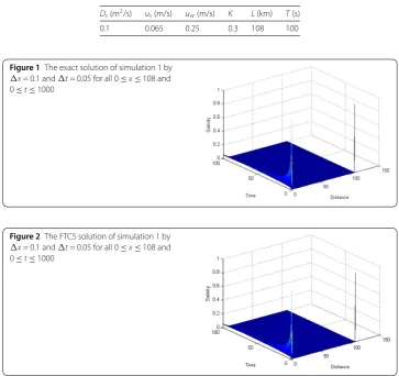
Table 2 Physical parameters of simulation 1
Ds(m2/s) us(m/s) uw(m/s) K L(km) T(s)
0.1 0.065 0.25 0.3 108 100
Figure 1The exact solution of simulation 1 by
x= 0.1 andt= 0.05 for all 0≤x≤108 and 0≤t≤1000
Figure 2The FTCS solution of simulation 1 by
x= 0.1 andt= 0.05 for all 0≤x≤108 and 0≤t≤1000
Table 3 The maximum absolute error defined byerrmax= max|˜c(xi,T) –c(xi,T)|for alli= 0, 1,. . .,N,
whereT= 10, 20, 30, and 40
T FTCS Saulyev
errmax errmax
10 5.9442×10⁻⁴ 5.1141×10⁻⁴
20 0.0044 0.0042
30 0.0083 0.0082
40 0.0107 0.0107
time is 100. Their physical parameters and given spacing are shown in Table2. In [11], the theoretical solution is given by
c(x,t) =√ 1 4t+ 1exp
–(x– 1 – (us–kuw)t)
2
D(4t+ 1)
. (23)
Figure 3The Saulyev solution of simulation 1 by
x= 0.1 andt= 0.05 for all 0≤x≤108 and 0≤t≤1000
Table 4 Physical parameters of simulation 2
Ds(m2/s) us(m/s) uw(m/s) K L(km) T(s)
0.1 0.065 0.3 0.3 108 100
0.1 0.065 0.25 0.3 108 100
0.1 0.065 0.2 0.3 108 100
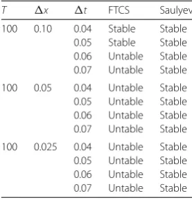
Table 5 Convergence of FTCS method and Saulyev method for some grid spacing
T x t FTCS Saulyev
100 0.10 0.04 Stable Stable 0.05 Stable Stable 0.06 Untable Stable 0.07 Untable Stable
100 0.05 0.04 Untable Stable 0.05 Untable Stable 0.06 Untable Stable 0.07 Untable Stable
100 0.025 0.04 Untable Stable 0.05 Untable Stable 0.06 Untable Stable 0.07 Untable Stable
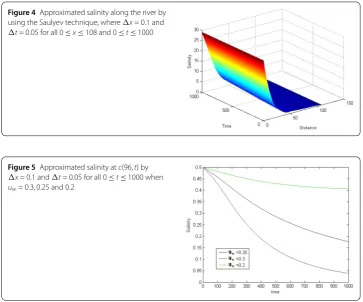
4.2 Simulation 2: the salinity is diluted by releasing the fresh water from a barrage dam with different flow velocities.
We consider a segment of a river with 108 km of length as shown in Table1. Assuming that the salinity diffusion coefficient is 0.1 m2/s, the salinity flow velocity is 0.065 m/s,
the ability percentage of fresh water dilution is 30%, and the given simulated station at any time is 1000. Their physical parameters and given spacing are shown in Table4. In this simulation, the Saulyev technique is used to approximate the solution since the tech-nique will always give stable solutions as shown in Table5. According to the good agree-ment of approximated solutions of the Saulyev method, the method in Eq. (23) is cho-sen to approximate the solution of the simulation. The several fresh water flow velocities
uw= 0.20, 0.25, 0.30 m/s from the barrage dam are simulated until the salinity level at the
Figure 4Approximated salinity along the river by using the Saulyev technique, wherex= 0.1 and
t= 0.05 for all 0≤x≤108 and 0≤t≤1000
Figure 5Approximated salinity atc(96,t) by
x= 0.1 andt= 0.05 for all 0≤t≤1000 when
uw= 0.3, 0.25 and 0.2
Table 6 Physical parameters of simulation 3
c(x,t) atS7 D(m2/s) us(m/s) uw(m/s) K T L(km) c(0,t)
>CST 0.1 0.065 0.25 0.3 1000 108 g(t)
<CST 0.1 0.065 0.205 0.3 1000 108 g(t)
4.3 Simulation 3: the salinity is diluted by releasing the fresh water from a barrage dam and changing flow velocities after the salinity comes to standard
We consider a segment of a river with 108 km of length as shown in Table1. Assuming that the salinity diffusion coefficient is 0.1 m2/s, the salinity flow velocity is 0.065 m/s, the
ability percentage of fresh water dilution is 30%, and the given simulated station at any time is 1000. Their physical parameters and given spacing are shown in Table6. Assume that there are eight monitoring stations along a considered river segment as shown in Table1. The controlled monitoring station is stationS7. We need to control the salinity
level at stationS7to be under the salinity standard levelCST = 0.3kg/m3. The salinity is
controlled by a process as follows:
(1) If the salinity level at stationS7c(96,t) >CST, then the fresh water will be released at a high speed from the barrage dam by controlled flow velocity.
(2) If the salinity level at stationS7c(96,t) <CST, then the fresh water will be released at a low speed level from the barrage dam.
We can obtain the approximated salinity level along the considered river segment as shown in Fig.6and Table7. The salinity level at several monitoring stationsS1,S5, andS7
Figure 6The numerical solution of simulation 2 by
x= 0.1 andt= 0.05 for all 0≤x≤108 and 0≤t≤1000
Table 7 Approximated salinityc(x,t) of simulation 2 for all monitoring stations
t S1 S2 S3 S4 S5 S6 S7 S8
1 12.1040 4.0187 2.0224 1.0978 0.7955 0.5316 0.4995 0.1444
5000 11.3456 3.6020 1.9844 1.0058 0.7667 0.4807 0.3844 0.0027
10,000 11.3391 3.6002 2.0397 1.0128 0.7476 0.4098 0.2993 0.0023
15,000 13.7382 4.4013 2.4788 1.1159 0.7704 0.3996 0.2987 0.0032
20,000 15.5617 5.3633 3.0060 1.2576 0.8025 0.3961 0.2983 0.0034
Figure 7Approximated salinity of simulation 2 at stationS1byx= 0.1 andt= 0.05 for all 0≤t≤1000
Figure 8Approximated salinity of simulation at stationS5byx= 0.1 andt= 0.05 for all 0≤t≤1000
4.4 Simulation 4: diluting the salinity of water by releasing fresh water before salinity water arrives at the pumping station
We consider a segment of a river with 108 km of length as shown in Table1. Assume that the salinity diffusion coefficient is 0.1 m2/s, the salinity flow velocity is 0.065 m/s, the ability
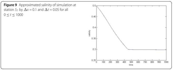
Figure 9Approximated salinity of simulation at stationS7byx= 0.1 andt= 0.05 for all 0≤t≤1000
Table 8 Physical parameters of simulation 2
c(x,t) atS5 D(m2/s) us(m/s) uw(m/s) K T L(km) c(0,t)
<CST 0.1 0.065 0 0.3 1000 108 g(t)
>CST 0.1 0.065 0.25 0.3 1000 108 g(t)
Figure 10 The numerical solution of simulation 3 by
x= 0.1 andt= 0.05 for all 0≤x≤108 and 0≤t≤1000
1000. Their physical parameters and given spacing are shown in Table8. Assume that there are eight monitoring stations along the considered river segment as shown in Table1. The controlled monitoring station is stationS7. We need to control the salinity level at station
S7before salinity level at station S7 is over the salinity standard levelCST = 0.05 kg/m3
for about three days. In this simulation, the Saulyev technique is used to approximate the solution since the technique will always give stable solutions. The salinity is controlled by a process as follows:
(1) If the salinity level at stationS5c(91,t) <CST, then the fresh water is released at a normal speed level from the barrage dam.
(2) If the salinity level a stationS5c(91,t) >CST, then the fresh water will be released at a high speed from the barrage dam which is used to control the salinity.
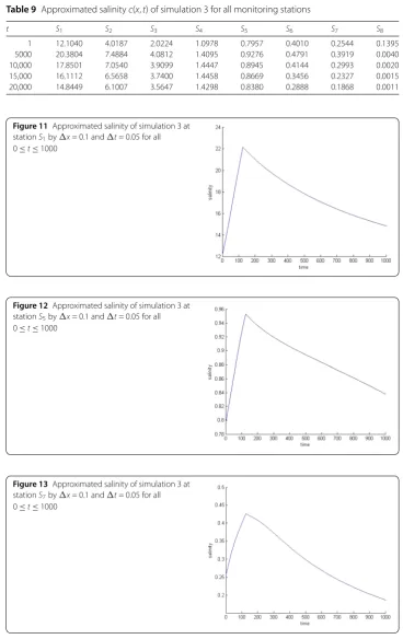
We can obtain the approximated salinity level along the considered river segment as shown in Table9and Fig.10. The salinity level at several monitoring stationsS1,S5, and
S7is shown in Figs.11,12, and13, respectively.
5 Discussion
Table 9 Approximated salinityc(x,t) of simulation 3 for all monitoring stations
t S1 S2 S3 S4 S5 S6 S7 S8
1 12.1040 4.0187 2.0224 1.0978 0.7957 0.4010 0.2544 0.1395
5000 20.3804 7.4884 4.0812 1.4095 0.9276 0.4791 0.3919 0.0040
10,000 17.8501 7.0540 3.9099 1.4447 0.8945 0.4144 0.2993 0.0020
15,000 16.1112 6.5658 3.7400 1.4458 0.8669 0.3456 0.2327 0.0015
20,000 14.8449 6.1007 3.5647 1.4298 0.8380 0.2888 0.1868 0.0011
Figure 11 Approximated salinity of simulation 3 at stationS1byx= 0.1 andt= 0.05 for all 0≤t≤1000
Figure 12 Approximated salinity of simulation 3 at stationS5byx= 0.1 andt= 0.05 for all 0≤t≤1000
Figure 13 Approximated salinity of simulation 3 at stationS7byx= 0.1 andt= 0.05 for all 0≤t≤1000
a salinity control process is simulated. The salinity is reduced, the salinity level comes to standard, after that we can decrease the fresh water flow velocity to maintain the salinity level at the standard level as shown in Fig.9. In simulation 4, a salinity control process is simulated. The salinity is reduced before the salinity level touches the standard salinity level. The proposed process can reduce the salinity level when the fresh water is released from the barrage dam at least amount as shown in Figs.11–13.
6 Conclusion
We have proposed a one-dimensional mathematical model of salinity measurement in a river with a barrage dam. The proposed model deals with salinity advection to a river and the fresh water flow from the barrage dam effects. The traditional forward time cen-tral space finite difference method is compared with the proposed Saulyev technique. The proposed Saulyev technique gives a stable solution in any grid spacing. The technique also gives accurately approximated solutions. The realistic problem is also simulated. The proposed simulation can be used in several realistic salinity measurements. In the salin-ity control aspect, the proposed process can reduce the salinsalin-ity level before the level is over the standard. The proposed numerical simulation can be applied in practical salinity control in a river with a barrage dam.
Funding
This paper is supported by the Centre of Excellence in Mathematics, the Commission on Higher Education, Thailand. The authors greatly appreciate valuable comments received from the referees.
Competing interests
The authors declare that they have no competing interests.
Authors’ contributions
All authors contributed equally to the writing of this paper. The authors read and approved the final manuscript.
Publisher’s Note
Springer Nature remains neutral with regard to jurisdictional claims in published maps and institutional affiliations.
Received: 30 January 2019 Accepted: 17 April 2019
References
1. Pochai, N., Tangmanee, S., Crane, L.J., Miller, J.J.H.: A mathematical model of water pollution control using the finite element method. In: Proceedings in Applied Mathematics and Mechanics, 27–31 March 2006, Berlin (2006) 2. Tabuenca, P., Vila, J., Cardona, J., Samartin, A.: Finite element simulation of dispersion in the Bay of Santander. Adv.
Eng. Softw.28, 313–332 (1997)
3. Pochai, N., Tangmanee, S., Crane, L.J., Miller, J.J.H.: A water quality computation in the uniform channel. J. Interdiscip. Math.11, 803–814 (2008)
4. Pochai, N.: A numerical computation of non-dimensional form of stream water quality model with hydrodynamic advection-dispersion-reaction equations. Nonlinear Anal. Hybrid Syst.13, 666–673 (2009)
5. Pochai, N.: A numerical computation of non-dimensional form of a nonlinear hydrodynamic model in a uniform reservoir. Nonlinear Anal. Hybrid Syst.3, 463–466 (2009)
6. Pochai, N.: Unconditional stable numerical techniques for a water-quality model in a non-uniform flow stream. Adv. Differ. Equ.2017, 286 (2017)
7. Thongtha, K., Kasemsuwan, J.: Analytical solution to a hydrodynamic model in an open uniform reservoir. Adv. Differ. Equ.2017, 149 (2017)
8. Nahian, M.A., Ahmed, A., Lazar, A.N., Hutton, C.W., Salehin, M., Streatfield, P.K.: Drinking water salinity associated health crisis in coastal Bangladesh. Elem. Sci. Ant.6, 2 (2018)
9. Suarez, D.L., Lebron, I.: Water quality criteria for irrigation with highly saline water. In: Towards the Rational Use of High Salinity Tolerant Plants, vol. 28, pp. 389–397 (1996)
10. Letey, J.: Relationship between salinity and efficient water use. Irrigation science. Irrig. Sci.14, 75–84 (1993) 11. Leewatchanakul, K.: Salinity intrusion in Chao Phraya river. PhD thesis, Chulalongkorn University (1988)
12. Grant, R.F.: Salinity water use and yield of maize: testing of the mathematical model ecosys. Plant Soil172, 389–397 (1995)
13. Chapra, S.C.: Surface Water-Quality Modeling. McGraw-Hill, New York (1997)
14. Pochai, N.: A numerical treatment of nondimensional form of water quality model in a nonuniform flow stream using Saulyev scheme. Math. Probl. Eng.2011, 1–16 (2011)