Volume 2009, Article ID 568570,11pages doi:10.1155/2009/568570
Research Article
Feedforward Data-Aided Phase Noise Estimation from
a DCT Basis Expansion
Jabran Bhatti and Marc Moeneclaey
Department of Telecommunications and Information Processing, Ghent University, 9000 Ghent, Belgium
Correspondence should be addressed to Marc Moeneclaey,[email protected]
Received 1 July 2008; Revised 5 November 2008; Accepted 25 December 2008
Recommended by Erchin Serpedin
This contribution deals with phase noise estimation from pilot symbols. The phase noise process is approximated by an expansion of discrete cosine transform (DCT) basis functions containing only a few terms.We propose a feedforward algorithm that estimates the DCT coefficients without requiring detailed knowledge about the phase noise statistics. We demonstrate that the resulting (linearized) mean-square phase estimation error consists of two contributions: a contribution from the additive noise, that equals the Cramer-Rao lower bound, and a noise independent contribution, that results from the phase noise modeling error. We investigate the effect of the symbol sequence length, the pilot symbol positions, the number of pilot symbols, and the number of estimated DCT coefficients on the estimation accuracy and on the corresponding bit error rate (BER). We propose a pilot symbol configuration allowing to estimate any number of DCT coefficients not exceeding the number of pilot symbols, providing a considerable performance improvement as compared to other pilot symbol configurations. For large block sizes, the DCT-based estimation algorithm substantially outperforms algorithms that estimate only the time-average or the linear trend of the carrier phase.
Copyright © 2009 J. Bhatti and M. Moeneclaey. This is an open access article distributed under the Creative Commons Attribution License, which permits unrestricted use, distribution, and reproduction in any medium, provided the original work is properly cited.
1. Introduction
Phase noise refers to random perturbations in the carrier phase, caused by imperfections in both transmitter and receiver oscillators. Compensation of this phase noise is critical since these disturbances can considerably degrade the system performance. The phase noise process typically has a low-pass spectrum [1]. A description of the characteristics of oscillator phase noise is given in [2]. Discrete-time processes that have a bandwidth which is considerably less than the sampling frequency can often be modeled as an expansion of suitable basis functions, that contains only a few terms. Such a basis expansion has been successfully applied in the context of channel estimation and equalization in wireless communications, where the coefficients of the channel impulse response are low-pass processes with a bandwidth that is limited by the Doppler frequency [3–5]. Several methods trying to tackle the phase noise problem exist.
(i) Designing oscillators operating at low-phase noise reduces the need of accurate phase noise compensation algorithms. This, however, leads to expensive oscillators which are difficult to integrate on chip [6–8].
(ii) Phase noise can be tracked by means of a feedback algorithm that operates according to the principle of the phase-locked loop (PLL). As feedback algorithms give rise to rather long acquisition transients, they are not well suited to burst transmission systems [9,10].
be short, in which case a high sensitivity to additive noise occurs.
(iv) Recently, iterative joint estimation and decod-ing/detection algorithms have been proposed that make use of the a priori statistics of the phase noise process. A factor graph approach for the estimation of the Markov-type phase noise has been presented in [12, 13], while in [14, 15] sequential Monte Carlo methods combined with Kalman filtering are used to perform detection in the presence of phase noise. These algorithms are computationally rather complex, prevent the use of off-the-shelf decoders, and assume detailed knowledge about the phase noise statistics at the receiver. Less complex iterative phase noise estimation algorithms based on Wiener filtering have been presented in [16], but still require knowledge about the phase noise autocorrelation function at the receiver.
In this contribution, we apply the basis expansion model to the problem of phase noise estimation from pilot symbols only, using the orthogonal basis functions from the discrete cosine transform (DCT). In contrast to the case of channel estimation, the phase noise does not enter the observa-tion model in a linear way. Section 2 presents the system description which includes the observation model and a general phase noise model. Also, the phase noise estimation algorithm, based on the estimation of only a few DCT coefficients, is derived. Section 3contains the performance analysis of the proposed algorithm in terms of the mean-square error (MSE) of the phase estimate. The behavior of the linearized model in the frequency domain is examined in Section 4. Analysis results are confirmed by computer simulations in Section 5, which consider both the mean-square phase estimation error and the associated bit error rate (BER) degradation.Section 6gives a complexity analysis of our algorithm. Conclusions are drawn inSection 7.
2. System Description
We consider the transmission of a block of K data symbols over an AWGN channel that is affected by phase noise. The resulting received signal is represented as
r(k)=a(k)ejθ(k)+w(k) for k=0,. . .,K−1, (1) where the index k refers to the kth symbol interval of lengthT,{a(k)}is a sequence of data symbols with symbol energy E[|a(k)|2] = E
s, the additive noise {w(k)} is a
sequence of i.i.d. zero-mean circularly symmetric complex-valued Gaussian random variables with E[|w(k)|2
] = N0, andθ(k) is a time-varying phase noise process with K×K
correlation matrixRθ. The symbol sequence{a(k)}contains
KP known pilot symbols at positions ki,i = 0,. . .,KP −1,
with constant magnitude|a(ki)|2=Es. From the observation
of the received signal at the pilot symbol positions ki,
an estimate θ(k) of the time-varying phase θ(k) is to be produced. This phase estimate will be used to rotate the received signal before data detection, that is, the detection of the data symbols is based on{z(k)} = {r(k)exp(−jθ(k))}. The detector is designed under the assumption of perfect carrier synchronization, that is,θ(k) = θ(k). For uncoded
transmission, the detection algorithm reduces to symbol-by-symbol detection:
with A denoting the symbol constellation. The phaseθ(k) can be represented as a weighed sum ofK basis functions over the interval [0,K−1]:
θ(k)=
K−1
n=0
xnψn(k), k=0,. . .,K−1. (3)
As θ(k) is essentially a low-pass process, it can be well approximated by the weighed sum of alimited numberN(
K) of suitable basis functions:
θ(k)≈
N−1
n=0
xnψn(k), k=0,. . .,K−1. (4)
In this contribution, we make use of the orthonormal discrete cosine transform (DCT) basis functions, that are defined as
As ψn(k) has its energy concentrated near the frequencies
n/2KTand−n/2KT, the DCT basis functions are well suited to represent a low-pass process by means of a small number of basis functions.
In the following, we produce from the observation {r(ki)}at the pilot symbol positionski, withi=0,. . .,KP−1,
an estimatexnof the coefficientsxn, withn =0,. . .,N−1,
using the phase model (4) with equality. The final estimate
noise contained in the observation, but also by a phase noise modeling error. Considering the observations (1) at instants
ki, and assuming that (4) holds with equality, we obtain
the instantskithat correspond to the pilot symbol positions.
Similarly, the nth column of the KP × N matrix ΨP is
obtained by subsampling thenth DCT basis functionψn(k).
Maximum likelihood estimation ofxfromrPresults in
xML=arg min
x rP−D(x)aP
2
. (9)
Asx enters the observationrP in a nonlinear way, the ML
estimate is not easily obtained. Therefore, we resort to a suboptimum ad hoc estimation of x, which is based on the argument (angle) of the complex-valued observations. However, as the function arg(z) reduces the argument ofz
to an interval [−π,π], taking arg(r(ki)) might give rise to
phase wrapping, especially when the time-average ofθ(k) is close to−πorπ. In order to reduce the probability of phase wrapping, we first rotate the observationrover an angleθavg that is close to the time-average ofθ(k), then we estimate the DCT coefficients of the fluctuationθ(k)−θavgand finally we
and constructrwith
(r)i=r
phase estimate is given by
Note from (13) that the estimation algorithm does not need specific knowledge about the phase noise process. Asr(ki)
from (11) can be viewed as a noisy version ofθ(ki)−θavg,
the phase estimate θfrom (13), or, equivalently, the phase estimateθ(k) from (6), can be interpreted as an interpolated version of the subsampled noisy phase trajectory. The estimation of the phase trajectory involves the inversion of theN×NmatrixΨPTΨP, which depends on the pilot symbol
positions{ki,i=0,. . .,KP−1}. Now, we point out that the
pilot symbol positions can be selected such thatΨPTΨP is
diagonal, or, equivalently, that theNcolumns of theKP×N
matrixΨPare orthogonal. Such selection of{ki}avoids the
need for matrix inversion in (12). Denoting by φn(i) the
orthonormal DCT basis functions of lengthKP, it is easily
verified that selecting{ki}such that
ki=iK
withIN denoting theN×Nidentity matrix. Equations (12)
and (13) then reduce to
(2d+1)i+d. The resulting pilot symbol configuration is suited for estimating any number of DCT coefficients not exceeding
KP. WhenKis not an odd multiple ofKP, rounding the
right-hand side of (14) to the nearest integer gives rise to pilot symbol positions that still yield an essentially diagonal matrix ΨPTΨPin which case the simplified equations (17) and (18)
can still be used.
3. Performance Analysis
As the observation vectorrP is a nonlinear function of the
carrier phase, an exact analytical performance analysis is not feasible. Instead, we will resort to a linearization of the argument function in (11) in order to obtain tractable results.
Linearization of the argument function yields
r(i)=argrki
zero-mean Gaussian random variables with varianceN0/2Es.
Note that (19) incorporates the true phaseθ(ki) instead of
the approximate model (4), so that our performance analysis will take the modeling error into account. In order that the linearization in (19) be valid, we need |θ(ki)−θavg| < π
(because|arg(z)|< π) and|w(ki)|2 Es; hence, the phase
noise fluctuations should not cause phase wrapping and
where (nP)i=nP(i), (θP)i=θ(ki), and theKP×KmatrixS
in which case the estimation error would be caused only by the additive noise.
As a performance measure of the estimation algorithm, we consider the mean-square error (MSE), defined as
MSE= 1
The first term in (24) denotes the contribution from the additive noise, whereas the second term in (24) constitutes an MSE floor, caused by the phase noise modeling error. The phase noise statistics affect the MSE floor through the autocorrelation matrix Rθ. The MSE floor decreases with
increasingN (because the modeling error is reduced when more DCT coefficients are taken into account), whereas the additive noise contribution to the MSE increases with N
(becauseNparameters need to be estimated). Hence, there is an optimum value ofNthat minimizes the MSE.
From the nonlinear observation model (7), which assumes that (4) holds with equality, we compute the Cramer-Rao lower bound on the MSE (23) resulting from any unbiased estimatexof the DCT coefficients ofθ(k):
MSE≥ 1
Ktrace
J−1. (26)
In (26),J denotes the Fisher information matrix related to the estimation ofxfrom (7), which is found to be
Combining (26) with (27) yields the following performance bound: rithm (13) yields the minimum possible (over all unbiased estimates) noise contribution to the MSE (assuming that the linearization of the observation model is valid).
When the pilot symbol positions {ki} are selected
according to (14), the Cramer-Rao bound (28) reduces to
MSE≥ N0
2Es
N KP
, (29)
which indicates that the sensitivity to additive noise increases with the number (N) of estimated DCT coefficients.
4. Frequency-Domain Analysis
After linearization, (20) relates the phase estimateθto the actual phaseθ and the additive noisenP. In the absence of
additive noise, the estimator can be viewed as a linear system that transformsθintoθby means of the transfer matrixMS. In order to analyze this system in the frequency domain, we consider an inputθnwith (θn)k=exp(j2πkn/K), that is,θn
contains only the frequencyn/K. We investigate the mean-square error MSEn between the input θn and the output
θ=MSθn; MSEnis given by (25), withRθreplaced byθnθHn,
where the superscriptHindicates conjugate transpose. Asθnis periodic innwith periodK, the same periodicity
holds for MSEn. Assuming the pilot symbol positions are
according to (14) with K = 105 and K p = 15, Figure 1 shows MSEnas a function ofn/K, withn/K in the interval
[−1/2, 1/2] andN=7. The behavior of MSEnis explained by
noting that subsamplingθnat the instantski(with spacing
KP) gives rise to aliasing. Frequenciesn/K and (n+KP)/K
yield the same subsampled phase trajectory. In the following discussion, the intervalsIKP andIN are defined as [−(KP− 1)/(2K), (KP−1)/(2K)] and [−(N−1)/(2K), (N−1)/(2K)],
respectively; note thatIN ⊂IKP.
(i) As the firstN basis functions of the DCT transform cover the frequency intervalIN, we getθn ≈θnand
resulting estimation error is the sum of two complex exponentials with frequenciesn/Kandn/K, yielding MSEn≈2. Whennis not inIN, we getθn ≈0 and
MSEn≈1.
It follows fromFigure 1that the estimator can be viewed as a low-pass system with bandwidth B = (N−1)/(2K). Basically, the frequency componentsn/Kofθwith|n/K|< B
are tracked by the estimator, whereas the components with |n/K|> Bcontribute to the MSE.
5. Simulation Results
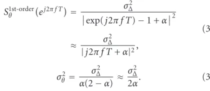
simulations. In our simulations, we will consider two types of phase noise, that is, Wiener phase noise and first-order phase noise. The (discrete time) first-order phase noise processθ(k) can be viewed as the output of a one-pole filter driven by white Gaussian noise:
θ(k+ 1)=(1−α)θ(k) +Δ(k), (30)
where {Δ(k)} is a sequence of i.i.d. zero-mean Gaussian random variables with varianceσ2
Δ. The corresponding phase noise power spectrum and phase noise variance are given by
S1st-order frequency of the power spectrum. The first-order phase noise models the phase instabilities of an oscillator signal that results from a phase-locked loop (PLL) circuit. The (discrete-time) Wiener phase noiseθ(k) is described by the following system equation:
θ(k+ 1)=θ(k) +Δ(k), k=0,. . .,K−2, (33)
where the initial phase noise value θ(0) is uniformly distributed in [−π,π] and Δ(k) has the same meaning as in (30). Hence, θ(k) can be viewed as the output of an integrator with a white noise input. From (33), it follows that the variance of the Wiener phase noise increases linearly with the time index k, which indicates that the process is nonstationary.
Comparing (33) and (30), it follows that the Wiener phase noise can be interpreted as a limiting case of first-order phase noise, in the limit forα → 0. Hence, one canformally
define the Wiener phase noise spectrum as the limit of the first-order spectrum (31); forα → 0, that the Wiener phase noise spectrum becomes unbounded at f =0, which is a consequence of the variance increasing linearly with time. In contrast, the complex envelope exp(jθ) of the oscillator signal can be shown to be a stationary process (with [1, the Lorentzian power spectrum]). The Wiener phase noise model is often used to describe the phase noise process of a free-running oscillator, although also more elaborate models exist, involving a phase noise spectrum that consists of a sum of terms of the formAmf−m, m=0,. . ., 4
[10, 17–19]. In order to reduce the strong low-frequency components of the phase noise resulting from a free-running oscillator, the oscillator is often incorporated in a PLL circuit;
0 First-order phase noise power spectrum Wiener phase noise power spectrum
Figure2: Power spectrum for Wiener phase noise and first-order phase noise.
a first-order PLL gives rise to the first-order phase noise process (30) [17].
Figure 2 shows the first-order phase noise power spec-trum, normalized by its value S0 at f = 0, as a function of the normalized frequency f / f3 dB, with f3 dB = α/(2πT); also displayed is the Wiener phase noise power spectrum (normalized by the same S0). As for both types of phase noise, the same value ofσ2
Δhas been used, both spectra have the same high-frequency content.
In the following simulations, Wiener phase noise is assumed, unless noted otherwise. First, we assume trans-mission of a block of lengthK = 105 symbols, consisting of KD = 90 uncoded QPSK data symbols and KP = 15
constant-energy pilot symbols that are inserted into the sequence according to (14).
1.E−04 1.E−03 1.E−02 1.E−01 1.E+ 00
MSE
(r
ad
2)
0 5 10 15 20 25
Es/N0(dB) N=1
N=4 N=10
CRB (N=1) CRB (N=4) CRB (N=10)
Figure 3: MSE in the absence of phase noise compared to the corresponding CRB.K=105, KP=15.
high values of Es/N0. For small Es/N0, the MSE exceeds
the CRB, which is in agreement with the fact that the linearized observation model from (19) is no longer accurate in the low-SNR region. Furthermore, it is confirmed that the contribution from the additive noise to the MSE is proportional to the number of estimated coefficientsN.
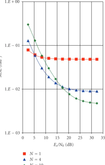
(ii)Figure 4shows the MSE as a function ofEs/N0 for
N = 1, 4 and 10, but this time in the presence of Wiener phase noise with σ2
Δ = 0.0027 rad2 (which corresponds to “strong” phase noise, with σΔ=3◦). We observe an MSE floor in the high-Es/N0 region, which can be reduced by increasing the numberN of estimated coefficients.Figure 4 also confirms that for lowEs/N0, the MSE increases whenN increases. This high-Es/N0and low-Es/N0behaviors indicate that for givenK,KP, andEs/N0, the MSE can be minimized by proper selection ofN.
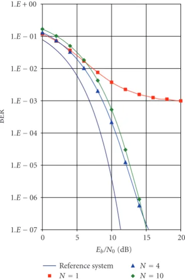
(iii)Figure 5shows the bit error rate (BER) as a function ofEb/N0(Ebis the energy per transmitted bit,Es=2(1−η)Eb
for QPSK) forN = 1, 4, and 10. The reference BER curve corresponds to a system with perfect synchronization and no pilot symbols (η = 0). We observe that for lowEb/N0, it is
sufficient to estimate only the time-average of the phase (i.e.,
N=1). Estimating a higher number of DCT coefficients can lead to a worse BER performance for lowEb/N0because the MSE of the phase estimate due to additive noise increases withN. At highEb/N0, a BER floor occurs which decreases
with increasing N, so in this region it becomes beneficial to estimate more than just one DCT coefficient. Hence, the
1.E−03 1.E−02 1.E−01 1.E+ 00
MSE
(r
ad
2)
0 5 10 15 20 25 30 35
Es/N0(dB) N=1
N=4 N=10
Figure4: MSE when Wiener phase noise withσΔ=3◦is present
K=105, KP=15.
optimal number of estimated coefficientsNopt will depend on the operatingEb/N0.
(iv) Figure 6 compares the BER degradations at BERref=10−4 resulting from Wiener phase noise and first-order phase noise; the value of σ2
Δ is the same for both phase noise processes, such that the Wiener phase noise spectrum and first-order phase noise spectrum are the same for large f. (The BER degradation caused by some impairment is characterized by the increase (in dB) ofEb/N0 (as compared to the case of no impairment) needed to maintain the BER at a specified reference level.) As the 3 dB frequencyα/(2πT) of the first-order phase noise is less than
BT, the frequency contents of the Wiener phase noise and the first-order phase noise outside the estimator bandwidth are essentially the same, and the corresponding BER curves are nearly coincident; this is in agreement with the analysis from Section 4, where we showed that the low-frequency components of the phase noise practically do not contribute to the phase error. It is also confirmed that there is an optimum value ofN that minimizes the BER degradation; this optimumNincreases withσΔ.
Next, we study the influence of the pilot symbol positions in the symbol sequence, assuming Wiener phase noise with σΔ=3◦. The following scenarios are considered (see
Figure 7), withKP=15.
(ii) All pilot symbols are located in the middle of the sequence (SCEN2).
(iii)KP/2pilot symbols are inserted at the beginning of
the sequence, the remainingKP/2pilot symbols are
placed at the end (SCEN3).
(iv) The KP pilot symbols are placed equidistantly at
positions{0,K/KP,..., (KP−1)K/KP}(SCEN4).
(v) We divide the total number of 15 pilot symbols into 3 clusters of 5 consecutive pilot symbols each. The 3 clusters are centered at the positions (14) that correspond toKP=3 (SCEN5).
(vi) We divide the total number of 15 pilot symbols into 5 clusters of 3 consecutive pilot symbols each. The 5 clusters are centered at the positions (14) that correspond toKP=5 (SCEN6).
Figure 8 shows the BER for each scenario with N = 4. We observe that SCEN2 and SCEN3 lead to essentially the same BER performance, that turns out to be very poor. The BER resulting from SCEN5 is slightly better, but still poor. Much better BER performance is obtained for SCEN1, SCEN4, and SCEN6, with SCEN1 yielding the best performance. The poor performance resulting from SCEN2, SCEN3, and SCEN5 comes from the poor conditioning of the 15×4 matrix ΨP, yielding very large values when
computing the inverse ofΨPTΨP. As the DCT basis functions ψ0(k),. . .,ψ3(k) change only slowly withk, SCEN2 yields a matrix ΨP with nearly identical rows, so it behaves like a
matrix of rank 1. Similarly, the matricesΨPthat correspond
to SCEN3 and SCEN5 behave like matrices of ranks 2 and 3, respectively. Hence, when the pilot symbols are placed in a number of clusters that are less than the number (N) of DCT coefficients to be estimated, poor performance results. For SCEN1, SCEN4, and SCEN6, the number of pilot symbol clusters exceedsN; the corresponding matricesΨPare
full-rank (full-rank =4), and good performance results. Note that SCEN1 and SCEN4 can cope with values of N up to KP,
whereas SCEN6 cannot handle values ofNin excess of 5. In the following, we investigate the influence of the number of pilot symbols on the MSE and the BER. The constant-energy pilot symbols are inserted into the data sequence according to (14). For (14) to hold, the block length
Kshould be an odd multiple of the number of pilot symbols
KP. We assume a total block lengthK = 105 and simulate
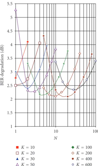
the BER and MSE forKP=7, 15, and 35.Figure 9shows the
BER degradation at BER=10−4with respect to the reference system, for a fixed ratioη=KP/K=20% and various values
of the block lengthK. The BER degradation−10 log(1−η) due to the insertion of pilot symbols (which amounts to 0.97 dB forη=0.2) is included. The following observation can be made.
(i) For given block sizeK, there is an optimum number
Noptof DCT coefficients to be estimated that minimizes the BER degradation. This is consistent with the observation that the MSE of the phase estimate can be minimized by a suitable choice ofN.
(ii) For very smallK,Nopt =1. The optimum valueNopt increases with increasingK because more DCT coefficients
1.E−07 1.E−06 1.E−05 1.E−04 1.E−03 1.E−02 1.E−01 1.E+ 00
BER
0 5 10 15 20
Eb/N0(dB)
Reference system N=1
N=4 N=10
Figure5: BER when Wiener phase noise withσΔ=3◦is present.
K=105, KP=15.
1 1.5 2 2.5 3 3.5
BER
d
eg
ra
dation
(dB)
1 3 5 7 9 11 13 15
N
Wiener phase noise (1) First-order phase noise (1) Wiener phase noise (2) First-order phase noise (2)
Figure6: BER degradation as a function of the number of estimated coefficientsN for Wiener phase noise and first-order phase noise withα =0.015. (1)σ2
Δ =0.0027 rad2; (2)σΔ2 =0.0015 rad2.K =
SCEN1
SCEN2
SCEN3
SCEN4
SCEN5
SCEN6
d 2d · · · 2d d
· · ·
KP
· · · · · ·
KP/2 KP/2
2d · · · 2d
Figure7: Pilot symbol insertion schemes.
1.E−05 1.E−04 1.E−03 1.E−02 1.E−01 1.E+ 00
BER
0 2 4 6 8 10 12
Eb/N0(dB)
SCEN1 SCEN2 SCEN3 SCEN4
SCEN5 SCEN6 Reference system
Figure8: BER for different pilot symbol placement scenarios.K= 105, KP=15, N=4.
are needed to model the phase fluctuations when K gets larger. KeepingN = 1 yields very large degradations when
Kincreases.
(iii) The BER degradation that corresponds toN =Nopt exhibits a (broad) minimum as a function ofK. As long as the fluctuation of θ(k) about its time-average is small, so that linearization of the argument function in (11) applies, the degradation decreases with increasing K because the numberKPof noisy observations of the phase noise increases
when the ratio KP/K is fixed. However, for too large K,
the fluctuation of the Wiener phase noise is so large that
1 1.5 2 2.5 3 3.5 4 4.5 5 5.5
BER
d
eg
ra
dation
(dB)
1 10 100
N
K=10 K=20 K=30 K=50
K=100 K=200 K=400 K=600
Figure9: BER degradation for BER=10−4as function ofN for variousK and fixed pilot symbol ratioη = KP/K = 20% and
σΔ=3◦.
linearization is no longer valid (for Wiener phase noise, we needKσ2
Δ 1 for the linearization to be accurate) and the resulting degradation increases with increasingK.
For the considered scenario, the minimum degradation occurs at (Kopt,Nopt) ≈ (400, 20) and amounts to about 2.1 dB. When the actual block size K exceeds Kopt, the degradation can be limited by dividing the block in subblocks of at mostKoptsymbols, and estimating the phase trajectory for each subblock separately.
Figure 10shows the BER degradation when (1)η=20% andσΔ=3◦and (2)η=10% andσΔ=2◦, for the following phase noise estimation algorithms.
(i) The proposed DCT-based algorithm with pilot sym-bol placement according to SCEN1 (14) and selection of the optimumN.
(ii) Estimation of only the time-average of the phase noise, with the pilot symbols arranged according to SCEN3.
(iii) The method from Luise et al. [11], with the pilot symbols arranged according to SCEN3. The phase noise over the total symbol block is approximated as a linear interpolation between the average phase values over the first and the second pilot symbol clusters .
0 1 2 3 4 5 6
BER
d
eg
ra
dation
(dB)
10 100 1000
Block lengthK Time-average, SCEN3 (1) DCT algorithm, SCEN1 (1) Luise et al. (1)
Time-average, SCEN3 (2) DCT algorithm, SCEN1 (2) Luise et al. (2)
Figure 10: Comparison of BER degradation for BER =10−4 as function ofK. (1)η=20% andσΔ=3◦; (2)η=10% andσΔ=2◦.
also estimates the time-average only (because N = 1 is optimum forK = 10); we observe that SCEN3 (with pilot symbols at positions 0 and 9) performs slightly better than the DCT-based algorithm (with pilot symbols at positions 2 and 7) for K = 10. However, when the block length is increased, the DCT algorithm that estimates multiple DCT coefficients outperforms both SCEN3 and Luise et al. and leads to a BER degradation that decreases with increasing K until an optimal value forKis reached.
6. Complexity Analysis
In order to assess the complexity of the proposed algo-rithm, we determine the number of complex multiplications required per symbol interval. The calculation of the second term in (18) requires the highest number of computations. This term can be evaluated in the following ways.
(1) In a first approach, (K/KP)ΨKΨPTr is calculated
via two matrix multiplications: firstΨPT (dimension N × KP) and r (dimension KP ×1) are multiplied and then
(K/KP)ΨK (dimensionK ×N)and ΨPTr (dimensionN×
1) are multiplied. The resulting complexity is of the order
O(NKP+KN)≈ O(KN), with the approximation holding
for K KP. Hence, the complexity per symbol interval
amounts toO(N).
0 5 10 15 20 25 30
C
o
mputational
comple
xit
y
10 100 1000
Block lengthK DCT approach 1 DCT approach 3 Luise et al.
Figure 11: Complexity comparison for the proposed algorithm (approaches 1 and 3) and for Luise et al. algorithm.
(2) In a second approach, (K/KP)ΨKΨPTris calculated
via a single-matrix multiplication: (K/KP)ΨKΨPT
(dimen-sionK×KP) andr(dimensionKP×1) are multiplied. Taking
into account that (K/KP)ΨKΨPT can be computed offline,
the resulting complexity per symbol isO(KP). AsN≤KP, the
first approach is to be preferred over the second approach. (3) The third approach exploits the fact that ΨK and ΨPare submatrices ofK×K andKP×KP DCT transform
matrices, respectively. Hence, the two matrix multiplications from the first approach can be replaced by an inverse DCT transform (size KP) followed by a DCT transform
(size K). AsK KP, the complexity of the size-K DCT
dominates. The DCT of a vector{s(0),s(1),. . .,s(K −1)} of length K can be obtained by calculating the discrete Fourier transform (DFT) of its even expansion {s(K − 1),. . .,s(1),s(0),s(0),s(1),. . .,s(K−1)}(note that the even expansion has length 2K). As the FFT algorithm used for calculating the DFT of length M has a computational complexity O(Mlog2(M)), the complexity of the size- K
DCT isO(2Klog2(2K)), yielding a complexity per symbol interval ofO(log2(4K2)).
The complexity per symbol interval of the phase noise estimation method used by Benvenuti et al. [11] is about
a smaller complexity than the proposed algorithm, but the latter algorithm outperforms the former, especially when the phase noise is strong. For the proposed algorithm, we notice that matrix multiplication according to the first approach leads to the lowest computational complexity for
K < 400. As K becomes larger than 400, calculation via FFT (third approach) is less complex. At the point (Kopt,Nopt)=(400, 20) yielding minimum BER degradation (seeFigure 9), the first and third approaches give rise to the same complexity.
7. Conclusions and Remarks
In this contribution, we have considered an ad hoc feed-forward data-aided phase noise estimation algorithm that is based on the estimation of only a few (N) coefficients of the DCT basis expansion of the time-varying phase. The algorithm does not require detailed knowledge about the phase noise statistics. Linearization of the observation model has indicated that the mean-square error of the resulting estimate consists of an additive noise contribution (that increases with N) and an MSE floor caused by the phase noise modeling error (that decreases with N). The noise contribution coincides with the Cramer-Rao lower bound.
These analytical findings have been confirmed by means of computer simulations. The influence of the position and number KP of pilot symbols inserted into the
sym-bol sequence has been investigated. Computer simulations were carried out for several pilot symbol configurations. Arranging the pilot symbols according to (14), such that the subsampled DCT basis functions remain orthogonal, reduces the BER degradation as compared to the case of a preamble/postamble or midamble pilot symbol arrangement with estimation of only the time-average; in addition, the configuration (14) allows to estimate up to KP DCT
coefficients with a reduced computational complexity. The BER degradation can be minimized by a suitable choice of block length K, the number KP of pilot symbols, and the
numberNof DCT coefficients to be estimated.
The considered DCT-based phase estimation algorithm makes use of the energy associated with the pilot symbols only. Further research will involve the incorporation of the DCT-based algorithm in an iterative phase noise estimation algorithm that exploits soft decisions about the data symbols, so that the resulting algorithm benefits from the energy associated with the data symbols as well. The performance and complexity of such an iterative algorithm will be investigated and compared to other iterative algorithms (such as those from [12–16]).
Acknowledgments
The authors wish to acknowledge the activity of the Network of Excellence in Wireless COMmunications (NEWCOM++) of the European Commission (Contract no. 216715) that motivated this work. This work is also supported by the FWO Project G.0047.06 Advanced space-time processing
techniques for communication through multiantenna sys-tems in realistic mobile channels.
References
[1] A. Demir, A. Mehrotra, and J. Roychowdhury, “Phase noise in oscillators: a unifying theory and numerical methods for characterization,”IEEE Transactions on Circuits and Systems I, vol. 47, no. 5, pp. 655–674, 2000.
[2] T. E. Parker, “Characteristics and sources of phase noise in stable oscillators,” inProceedings of the 41st Annual Frequency Control Symposium, pp. 99–110, Philadelphia, Pa, USA, May 1987.
[3] G. B. Giannakis and C. Tepedelenlioglu, “Basis expansion models and diversity techniques for blind identification and equalization of time-varying channels,” Proceedings of the IEEE, vol. 86, no. 10, pp. 1969–1986, 1998.
[4] J. K. Tugnait and W. Luo, “Blind space-time multiuser channel estimation in time-varying DS-CDMA systems,”IEEE Transactions on Vehicular Technology, vol. 55, no. 1, pp. 207– 218, 2006.
[5] O. Rousseaux, G. Leus, and M. Moonen, “Estimation and equalization of doubly selective channels using known symbol padding,”IEEE Transactions on Signal Processing, vol. 54, no. 3, pp. 979–990, 2006.
[6] J.-C. Nallatamby, M. Prigent, E. Vaury, A. Laloue, M. Camiade, and J. Obregon, “Low phase noise operation of microwave oscillator circuits,” IEEE Transactions on Ultrasonics, Ferro-electrics and Frequency Control, vol. 47, no. 2, pp. 411–420, 2000.
[7] J. Mukherjee, “Optimizing MOSFET channel width for low phase noise in LC oscillators,” in Proceedings of the 50th Midwest Symposium on Circuits and Systems (MWSCAS ’07), pp. 610–613, Montreal, Canada, August 2007.
[8] D. Y. Jung and C. S. Park, “Power efficient Ka-band low phase noise VCO in 0.13μm CMOS,”Electronics Letters, vol. 44, no. 10, pp. 628–630, 2008.
[9] H. Meyr, M. Moeneclaey, and S. Fechtel,Digital Communica-tion Receivers: SynchronizaCommunica-tion, Channel EstimaCommunica-tion, and Signal Processing, Wiley Series in Telecommunications and Signal Processing, John Wiley & Sons, New York, NY, USA, 1998. [10] U. Mengali and A. N. D’Andrea,Synchronization Techniques
for Digital Receivers, Plenum Press, New York, NY, USA, 1997. [11] L. Benvenuti, L. Giugno, V. Lottici, and M. Luise, “Code-aware carrier phase noise compensation on turbo-coded spectrally-efficient high-order modulations,” in Proceedings of the 8th International Workshop on Signal Processing for Space Communications (SPSC ’03), pp. 177–184, Catania, Italy, September 2003.
[12] G. Colavolpe, A. Barbieri, and G. Caire, “Algorithms for iterative decoding in the presence of strong phase noise,”IEEE Journal on Selected Areas in Communications, vol. 23, no. 9, pp. 1748–1757, 2005.
[13] J. Dauwels and H.-A. Loeliger, “Phase estimation by message passing,” inProceedings of the IEEE International Conference on Communications (ICC ’04), vol. 1, pp. 523–527, Paris, France, June 2004.
[15] E. Panayırcı, H. A. C¸ırpan, M. Moeneclaey, and N. Noels, “Blind-phase noise estimation in OFDM systems by sequential Monte Carlo method,”European Transactions on Telecommu-nications, vol. 17, no. 6, pp. 685–693, 2006.
[16] S. Godtmann, N. Hadaschik, A. Pollok, G. Ascheid, and H. Meyr, “Iterative code-aided phase noise synchronization based on the LMMSE criterion,” inProceedings of the 8th IEEE Signal Processing Advances in Wireless Communications (SPAWC ’07), pp. 1–5, Helsinki, Finland, June 2007.
[17] D. Petrovic, W. Rave, and G. Fettweis, “Effects of phase noise on OFDM systems with and without PLL: characterization and compensation,” IEEE Transactions on Communications, vol. 55, no. 8, pp. 1607–1616, 2007.
[18] ETSI, “Digital video broadcasting (dvb), second generation framing structure, channel coding and modulation systems for broadcasting, interactive services, news gathering and other broadband satellite applications”.