R E S E A R C H
Open Access
Simultaneous power control and power
management algorithm with sector-shaped
topology for wireless sensor networks
Mohsen Nickray
1, Ali Afzali-Kusha
1*and Riku Jäntti
2Abstract
In this paper, we propose a topology control technique to reduce the energy consumption of wireless sensor networks (WSNs). The technique makes use of both power control and power management methods. The algorithm uses the power management technique to put as many idle nodes as possible into the sleep mode while invoking the power control method to adjust the transmission range of the active nodes. On the contrary to earlier works in which both of these methods were used separately, in this algorithm, they are utilized simultaneously to decide about the sleep nodes and the ranges of active nodes. It is an approximation algorithm which is called simultaneous power control and power management algorithm (SPCPM). The performance bound of this centralized algorithm is determined analytically. Then, to make the proposed method practical for WSNs, a distributed algorithm based on SPCPM is introduced. To assess the efficiency of the proposed algorithm, we compare its average energy consumption with those of three existing topology control algorithms for a sector-based WSN. The simulation results which were obtained for different numbers of transmitting sensor nodes reveal less average energy consumptions for SPCPM compared to other algorithms.
Keywords:Power management; Power control; Wireless communication; Wireless sensor network; Network and architecture design; Low energy consumption
1 Introduction
Recent advances in wireless and electronic technologies have led to the emergence of wireless sensor networks (WSNs) with large-scale nodes. They are used in a wide spectrum of applications from industrial and military ap-plications to health and environmental monitoring. In these kinds of networks, different small-size sensor types are deployed in the area to monitor, e.g., temperature, motion, noise, and seismic activities. A good survey of WSNs is presented in [1] and [2]. The sensors are wire-less nodes that transmit the collected data (hop by hop) to a central station called base station or SINK node. Due to critical limitations of the node energy resources (e.g., battery), the nodes should minimize the energy consumption during their computation and communica-tion. Therefore, low-power algorithms for WSNs are of prime interest. Among different WSN types,
sector-shaped networks, where all the nodes send their data to a single base station, are the most common. They have various applications such as health monitoring, data gathering, and surveillance [3-5]. There have been sev-eral research efforts on reducing the ovsev-erall transmission power of sector-shaped networks [5-10]. The efforts may be divided into two categories of power control and power management techniques. The key idea of the power control techniques is that instead of transmitting using the maximum power, the nodes in a WSN collab-oratively reduce their transmission power by adjusting their transmission range while preserving some required properties (e.g., connectivity) [6-16]. The power control algorithms focus on reducing the power consumption when the nodes transmit or receive data in transmit and receive modes, respectively. Additionally, WSN nodes have a listen mode in which, while they are idle, they consume energy. The energy is comparable to the energy consumed in the other two modes. To reduce the energy consumption, the radio of the nodes in this mode may be turned off when they are not in use [17-20]. Turning * Correspondence:[email protected]
1
Nanoelectronic Center of Excellence, School of Electrical and Computer Engineering, University of Tehran, P.O. Box 14395-515, Tehran, Iran Full list of author information is available at the end of the article
off the radios when they are not in use is the basic idea of power management algorithms. Both of these tech-niques reside in the general category of the topology control algorithms.
It is expected that if these two types of techniques are invoked in coherence with each other in an algorithm, higher energy preservation will be achieved. This may be justified by noting that in this algorithm, the reduction of the energy consumptions of all the transmission, re-ceive, and idle states are considered simultaneously. The energy conservation of wireless sensor networks may be considered as an optimization problem where the energy consumptions of different sources should be minimized. For this problem, each of the power control and power management algorithms may be used. Depending on the network load, one of these algorithms is used for the en-ergy optimization. When the network load is low, the energy consumption of the network is dominated by the energy consumed by nodes in the idle state. For these loads, it is expected that fewer active (awake) nodes with long communication ranges lead to more energy conser-vation. In these cases, the power management algorithm should have a more determining role. In the cases where the network load is high, more active nodes with short communication ranges provide a better energy effi-ciency, and hence, the power control algorithm should play a major role in the optimization process. In this work, we propose an algorithm which integrates both of these techniques into one efficient algorithm.
1.1 Our contributions
In this paper, we make the following contributions. First, we present an analysis which shows that both the power control and power management techniques should be in-voked in coherence to enhance the energy preservation of WSNs. Then, we introduce an approximation algo-rithm provable performance bound which is analytically shown. Finally, based on this centralized algorithm, we propose a practical distributed algorithm whose key ad-vantages are given in the following:
– Its power management technique considers both time and space dimensions.
– It makes use of both power management and power control approaches simultaneously without giving any priority to any of them.
The rest of the paper is organized as follows. In Section 2, we briefly review the related works while Section 3 de-scribes the network topology along with the energy model which is used in our study. In Section 4, we use an example to show the dependency of the minimum en-ergy consumption to the network data traffic. In Section 5, we describe the proposed centralized Simultaneous
Power Control and Power Management (SPCPM) algo-rithm in detail and compare its efficiency with similar techniques reported in the literature. Section 6 is de-voted to the distributed SPCPM, and its performance is compared to those of existing techniques. Finally, the paper is concluded in Section 7.
2 Related works
In this section, we briefly review some of the previous works in the area of energy preservation of WSNs. These may be classified into two categories of power control and power management algorithms. The features of the algorithms are discussed while the main difference of our approach compared to these works is described at the end of the section.
2.1 Power control
Power control algorithms adjust the transmission power without adversely affecting desirable properties of the network (e.g., connectivity). Several empirical studies show that existing topology control solutions, which use static transmission power, transmission range, and link quality, might not be effective in the physical world (see, e.g., [21,22]). The authors in [22] propose a selective single-relay cooperative scheme, combining selective-relaycooperative communication with physical layer power control. Based on the medium access control (MAC) layer RTS-CTS signaling, a set of potential re-lays compute individually the required transmission power to participate in the cooperative communication. Based on the theory of stochastic fictitious play (SFP), a reinforcement learning algorithm to schedule each node’s power level is proposed in [23]. Also, a transmis-sion power self optimization (TPSO) technique is pre-sented in [24]. It basically consists of an algorithm able to guarantee the connectivity as well as an equally high Quality of Service (QoS) concentrating on the efficiency of WSNs, while optimizing the necessary transmission for data communication in each node.
surveys on the power control techniques in WSNs, one may see, e.g., [25-27].
2.2 Power management
Power management algorithms focus on turning off the radios of the nodes which are not in use. There are two basic approaches, namely, scheduling-based [17], [18] and backbone-based sleep management [13,20]. In [28], a systematic and comprehensive survey of the power management schemes is presented. In the scheduling-based approaches, nodes turn on their radios only in scheduled slots. Backbone-based sleep management can improve network performance by maintaining a back-bone composed of a small number of active nodes, while scheduling the other nodes to be active for small periods of time to conserve energy. From another aspect, the techniques may be divided based on the dimension that they use for the power management. The dimensions include node (e.g., [29]) or time (e.g., [13,20]). The ap-proaches based on the node dimension, such as geograph-ical adaptive fidelity (GAF) [29], mainly focus on detecting redundant nodes which can be turned off. In this algo-rithm, the network is divided into small square grids whose sizes are equal and fixed. All the nodes in a grid have the same routing role where at any time only one node is active and all the other nodes are in the sleep mode. The sleeping nodes periodically switch to the listen mode to guarantee that in each grid at least one node stays on. The algorithms based on the time dimension concentrate only on detecting the time when the nodes are idle and can be turned off [13,20]. In SPAN [13], a subset of nodes is adaptively selected to form a multi-hop forwarding backbone. The subset nodes, called coordina-tors, carry all the traffic of the network causing the ener-gies of the other nodes which are in the sleep mode to be conserved. A technique, which is called STEM, defines two ‘transfer’and ‘monitoring’states for the nodes [20]. The approach is based on the fact that most of the time the sensor network is only monitoring its environment, waiting for an event to happen. In this state, the nodes
can be asleep and the radio can be off. When an event is detected, the node becomes awake, changing its state to the transfer state.
2.3 Unified power control and power management algorithm
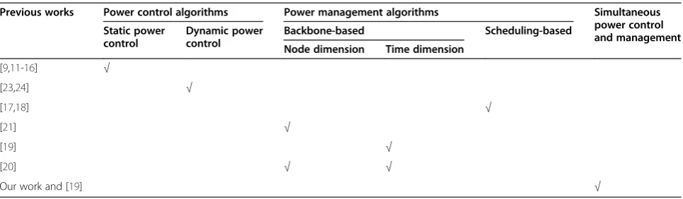
None of the power control or power management approaches optimizes the energy consumption of all the radio states. The power control techniques reduce the transmission energy of wireless nodes and do not consider the energy consumed during the idle state. The power man-agement algorithms reduce the energy dissipation in the idle state while not considering the energy consumptions of the transmit and receive states. It has been shown that for anad hocnetwork, when the network traffic is high, power control algorithms are effective while when the traffic is low, the use of power management algorithms provide us with more energy conservation [30,31]. In this work, we show that these findings hold true for a sector-shaped WSN too. Based on these facts, in this paper, we suggest a unified algorithm which makes a coherent use of both power con-trol and power management algorithms to minimize the energy consumption both in the idle and transmit/receive states. In our algorithm, we use a cell-based approach simi-lar to GAF. In our method, in addition to different forms of the cells, the transmission ranges of the nodes are adjusted dynamically. To the best of our knowledge, authors in [19] present the only similar approach. This approach is based on a joint duty-cycle optimization and transmission power control. By simultaneously adapting both parameters, the node can maximize the number of transmitted packets while respecting the limited and time-varying amount of available energy. Table 1 summarizes and makes a comparison between the related works and proposed algorithm in this work.
3 Network topology and energy model
3.1 Network topology
In a typical wireless sensor network, data flows toward the base station, and hence, the network area may be
Table 1 Comparison between the previous works and proposed algorithm in this work
Previous works Power control algorithms Power management algorithms Simultaneous power control and management Static power
control
Dynamic power control
Backbone-based Scheduling-based
Node dimension Time dimension
[9,11-16] √
[23,24] √
[17,18] √
[21] √
[19] √
[20] √ √
assumed as a sector-shaped area [8,10]. Similar to [9], in this work, the whole area is divided into some cells with the same area. We model the network area de-noted by ψ(α,R,N,K) using a sector with the angle of α and radiusRwhich is divided intoNcells andK annu-luses. Figure 1 shows ψ(π/6,R,16,4) which contains 4 annuluses and 16 cells with the angle of π/6. A sector area is divided into ring slices with the same ring width which are called network annulus. The areas of these network annuluses are not equal. Each network annulus may be divided into network cells with equal areas. Each annulus i may be divided into 2i-1 cells with the same area [9]. Figure 1 shows the network ψ(π/6,R,16,4) where each network annulus has been divided into net-work cells with equal areas.
3.2 Energy model
For the energy model, we adopt the first-order radio model described using [32,33]. Imagine u transmit data to node v. The energies consumed in the transmit state (Etx(d)) and receive state (Erx(d)) (transmit and receive energies, respectively) for a linear communication as a function of the distance (d) are, respectively, given by:
Etxð Þ ¼d Etxe þEr:d uð ;vÞα ð1Þ
Erxð Þ ¼d Erxe ð2Þ
where d(u,v) is the distance between transmitter u and receiverv,Etxe and Erxe are the is the energy consumed by the corresponding electronic circuits, Er is the energy
consumed by the power amplifier, andαis the path loss factor. In this work, we assume thatEtxe ¼Erxe ¼Ee.
4 Illustrating example
In this section, we illustrate the basic idea of our approach using a simple example. For the network shown in Figure 1, consider that the node A has some reports for the SINK node. The energy consumption used to transmit the data of the node includes the ener-gies dissipated in each of the transmit, receive, idle, and sleep states. The average energy consumptions are denoted by Etx(d), Erx, Eid, and Es, respectively. As
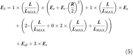
Figure 1 shows, the nodesA,B,C, andDare located in annuluses 4 to 1, respectively. Figure 1 shows three scenarios to transmit information to the SINK node. In one scenario (black arrows), first, the nodeA communi-cates with the node B, then the node Bcommunicates with the nodeC, and after that, the nodeCtransmit the data to the nodeD, and finally, the nodeDdelivers the data to the SINK node all using a transmission range of R/4. In another scenario (blue arrows), the nodeA com-municates with the nodeCand then the node C delivers the data to the SINK node both using a transmission range of R/2. The nodes B and D remain in the sleep state in this scheme. In the third scenario (red arrow), the node A directly delivers the reports to the SINK node using a transmission range of R. In this scenario the nodes B, C, and D remain in the sleep state. We denote the average energy consumptions of these three scenarios as E1, E2, and E3, respectively. Ei denotes the
sum of average energy consumption of all network nodes in scenario i. These energies may be obtained from: Figure 1Networkψ(π/6,R,16,4) which contains 4 annuluses and 16
E3¼1
L LMAX
EeþEr:
R 2
2!
þ1 L
LMAX
Ee
þ 2− L
LMAXþ
02 L
LMAX
þ L
LMAX
!
Eidþ3Es
ð5Þ
Each term on the right hand side of the equations is the product of the energy consumption in a state and the time fraction that the nodes operate in that state. For example, the first term ofE2 is the transmit energy of the nodes A and C with a transmission range ofR/2 andL/LMAXis the time fraction that these nodes operate
in the transmission state. Note that we have assumed that transmit and receive times are linearly proportional to the packet length, LMAX is the maximum packet
length that a node can transmit during one period, and Lis the length of the packet being transmitted. Since we have two nodes which take part in the packet transmis-sion, a coefficient of two has been used. The second term corresponds to the receive energies of the node C and the SINK node. The third term is associated with the energy consumed when the nodes A and C as well as the SINK node are in the idle state. The coefficient
(3-4 ×L/LMAX) is the fraction of time that these nodes
are in the idle state (e.g., for the nodeC, the fraction is (1-2 × L/LMAX). The forth term is the energy
con-sumed by the nodes in the sleep state. For this term, since the nodesBandDare in the sleep states, the co-efficient is two. Figure 2 part b depicts the terms of E2 in details.
In Figure 2 part a, we have plotted E1, E2, and E3
ver-sus different packet sizes of the source node. The results have been obtained assuming LMAX, R, Er, Eid, Ee, Es,
and α to be 500 bytes, 400 m, 0.01 nj/bit/m2, 50 nj/bit, 50 nj/bit, 12.5 pj/bit, and 2, respectively [34]. As the figure shows, when the network load is low, e.g., the packet size is 25 bytes, the minimum energy consumption will be achieved if the third scenario is used. In this scenario, the node A transmits data directly to the SINK node with the maximum transmission range while the other nodes are in the sleep state. When the network load is high, e.g., the packet size is more than 150 bytes, the first scenario will preserve energy more. For the medium range of traffic, e.g., the packet size of 80 bytes, the second scenario will lead to the minimum energy consumption.
As this example shows, when the network load is low, the energy consumption of the network is dominated by the idle energy. Therefore, scheduling more nodes to be in the sleep mode (power management task) with a long
transmission range for the active nodes (power control task) will preserve more energy. When the load is high, the transmit energy dominates the energy consumption of the network. For this case, scheduling more nodes in the active mode with short transmission ranges will pre-serve more energy. Since the nodes B, C, and D first should receive the data and then relay it, they can have, at most, one half of the active period for receiving the packet and the other half of the period for transmitting the packet. Therefore,L≤LMAX/2 orL/LMAX≤1/2. For
this reason, in the case of the example discussed in Figure 2, we assumed LMAX= 500 bytes × 8 bits = 4,000
bits and hence we plotted the energy consumptions ver-susLin the range of 50 to 2,000 bits.
We use the ratioL/LMAXto denote the proportion of the
network cycle time that is used by a node to transmit its data. This notation is only valid when the transmission rate is constant for all the nodes. Otherwise,L/LMAXshould be
replaced by node transmission time divided by the network cycle period.
5 Proposed algorithm
5.1 Problem definition
In this section, we state the problem which is minimiz-ing the energy consumption of the sector-shaped wire-less sensor networks. We define our problem like [20]. Let us assume that we have a set of traffic demands de-noted by f(si) where si is the ith sensor source node which has some data to report to the SINK node. t(si)
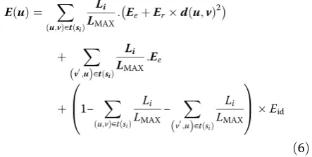
shows the set of the edges used for transmitting data from the source sito the SINK node. Our problem is to find a subnet from our network nodes satisfying the traf-fic demands with the minimum energy consumption. Obviously, minimizing the total energy consumption may be achieved through minimizing the average energy consumption. The average energy consumption of node umay be computed as:
E uð Þ ¼ X
Here, the first summation in the first line is performed on all the nodes (v) that the node u transmit packet to them, and the second summation is performed on all the nodes (v’) which they transmit to the node u. The average energy consumption of the node u is the weighted average of the transmit, receive, and idle
energy consumptions. Also, since the energy dissipation of the node in the sleep state is very small, it has been ignored in the calculations [30].
Problem definition: Given a sector-shaped network which is represented by graph G(V,E) (with vertices V and edges E) and a set of traffic demands denoted by t(si), find a subgraphG'(V',E') such that the total average
energy consumption E(G') is minimal. This energy is given by:
From the above formulation, we can see that each node has a fixed cost of Wc. Also, for each edge (u,v), the cost isWv(u,v) which is independent from the packet size. The packet size (proportional to the traffic load) has been entered in the calculation using a data fraction factor denoted byfi.
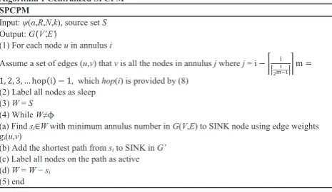
5.2 Centralized SPCPM
In this section, we introduce an approximation algo-rithm called SPCPM to maximize the energy preserva-tion of a sector-shaped wireless sensor network. In this algorithm, based on a combined cost function, the algo-rithm decides about the state of nodes and the transmis-sion range of the active nodes simultaneously.
5.2.1 A. Algorithm description
equal hop distances may not be possible which in these cases, one of the hop distances will become one hop smaller than the others. For example, the node B in Figure 1, may take the route B →C→SINK in a two-hop scenario. As will be discussed in Section 6, the assumption of equal hop distances does not considerably affect the efficacy of the algorithm.
The number of different scenarios (inter-hop dis-tances) for the node in the annulusimay be determined from:
hopð Þ ¼i log2iþ1 ð8Þ
Assume that the nodeuin the annulusihasjdifferent scenarios which we denote them by sce(1) to sce(j). The number of hops for each sce(m) (symbolized by |sce(m)|) is calculated from:
jsceð Þj ¼m ⌈i=2m−1⌉wherem¼1;2;3;…;j
ð9Þ
Also, the annulus number for the next hop of sce(j) is calculated from:
Annulus Number of Next HOPð Þi;j
¼Annulus Number of Current HOP–i=jsceð Þjj
As an example, consider the network of ψ(α,R,64,8). For this network, the number of transmission scenarios for a node in annulus 7 is 4 where the numbers of hops for these four scenarios will be 7, 4, 2, and 1. Consider-ing sce(2), the sequence of hops identified by the annu-lus number are 7 (the source node), 5,3, 1, and 0 (the SINK node) (|sce(2)| = 4).
Having found G, in the next step, we assume that all the nodes are in the sleep state. Let us use a set denoted by W for the remaining source nodes which we should find a route for connecting them to the base station. This set is initialized to the set of all the source nodes (S). The routes are determined by finding the shortest path from each source to the SINK node such that the energy is minimized. From G, we have all the possible routes to the base station. In the iteration i, SPCPM
selects the shortest path from G for connecting the source i to the SINK node using a weight function gi. Each weight functiongi(u,v) defines the cost of using the edge (u,v) for transferring the data of the sourcesito the base station. Obviously, the cost should depend on the data fraction (fi) of the source andWvbased on Equation (7). On the other hand, based on Equation (7), in the ex-pression for the energy, there is a constant (independent fromfi) energy cost for each node. Based on this obser-vation, we should add this cost once for any node whose state is changed from sleep to active. Therefore, the weight function for each edge (u,v) is defined as:
giðu;vÞ ¼ fiWvðu;vÞ þWcwhen u is sleep
fiWvðu;vÞwhen u is active
ð10Þ
After finding the shortest path for the iteration i, we set the state of all the nodes on this path to active. The output of SPCPM is the set of all the shortest paths found for all the iterations and the set of all the active nodes (G’(V’,E’)). It is apparent that the nodes which are not selected as active remain in the sleep state.
In Figure 3, we demonstrate how the centralized SPCPM works. For this example, we have a network with two annuluses and four cells (Figure 3a). Figure 3b shows G(V,E) which is obtained in part 1 of the algo-rithm. There are two sources which are S(1) and S(2) with data fractions of 0.1 and 0.2, respectively. The num-bers shown next to the edges in Figure 3b correspond to the values of Wv for the corresponding edges. Also, we have assumed Wc = 1. The results of the two iterations of the algorithm (corresponding to the two source nodes) are plotted in Figure 3c,d, where the numbers next to the edges are the weight functions of the source node. Note that, in each iteration, the weight of each edge is updated based on the data fraction as well as the change in the set of active nodes. Using Equation (7), we obtain the total average energy consumption for this example as 4.2.
5.2.2 B. SPCPM algorithm analysis
nodes in G, respectively. In the case of considering all pos-sible routes, the complexity increases to O(|S|.log|E|.log|V|) (see Equations (8)-(9)).
To calculate the approximation ratio of the algorithm, we follow the same approach as the one given in [30]. Let us define a set of weight functionciandhias:
ci¼fiWvðu;vÞ ð11Þ
hi¼WcþfiWvðu;vÞ ð12Þ
where ci(u,v) represents the cost of the edge (u,v) when the data of the source sitravels from the node uto the node v. The proposed algorithm finds the shortest path from each source to the SINK node. The cost (average energy) for the path from the sourcesito the SINK node (SN) is denoted by Ex
Gðsi;SNÞ under the weight function
x. Based on these notations, Equation (7) maybe expressed as:
Theorem: The approximation ratio of the algorithm SPCPM is not greater than:j jSj jVj j0K.
represent the total costs of G'
found by SPCPM using the weight function gi(u,v) and the optimal solution given by Equation (13), respectively. To obtain the approximation ratio, let us first start with the SPCPM algorithm when the weight function hi(u,v) is used. Sincegi≤ hi, the total cost of the shortest paths from all the sources to the SINK node in G' with the weight gi is greater than the one with the weight hi. Therefore, one may write: the weight function (regardless of the current state of the node being active or sleep), and hence, may be counted several times for each node inG'. Note that the maximum number ofWc which should be added to the total cost is |S|. |K|. The reason is that there are |S| sources where, in the worst case, there should be one node from each annulus on the path from each source to the SINK node. The cell configuration in our algo-rithm is such that each route uses at most one node from each annulus. Thus, one may write:
X ity and based on Equations (7) and (13), one may write:
X
Then, from Equations (14) and (17), we have:
E G0 ≤j j S j jK
Therefore, the approximation ratio of SPCPM, in the worst case, isj jSj jVj j0K.
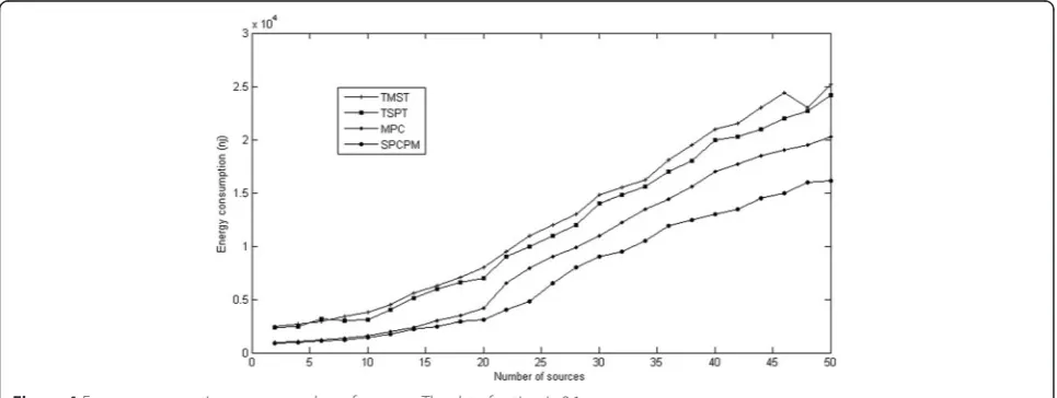
5.3 Performance evaluation
Spanning Tree (TMST) [10], Transmission power Shortest Path Tree (TSPT) [36], and Minimum Power Configuration (MPC) [30]. All the algorithms were implemented in MATLAB. The first two algorithms are basic topology con-trol methods while the last algorithm is similar to the SPCPM technique considering the minimization of both idle and transmit/receive energies. The TMST algorithm finds the minimum spanning tree of the network where each edge is weighed by the transmission power of the transmitting node. The TSPT technique finds the shortest path tree of the network when each edge is weighted by the transmission power. In the MPC algorithm which is more efficient compared to the two previous ones, each edge is weighted by a combination of the transmission and idle powers of the node. The parameters LMAX, R, Er, Eid, Ee, and
Esin our simulation were assumed to be 500 bytes, 400 m,
0.01 nj/bit/m2, 50 nj/bit, 50 nj/bit, and 12.5 pj/bit, respect-ively [34]. We assumed that 100 nodes were randomly distributed in the sector-shaped area with R = 800 m andα=π/4.
The total energy consumption of the network when the number of sources (|S|) varies from 1 to 50 is shown in Figure 4. The data fraction was assumed to be 0.1. The results shown in this figure reveal that MPC and SPCPM provide considerably higher energy preserva-tions compared to TSPT and TMST. This may be justi-fied by noting that these two techniques consider both the transmission and idle powers while TSPT and TMST ignore the idle power. The better performance of SPCPM compared to MPC could be attributed to two facts. First, the approximation for MPC (|S|) is higher than that for SPCPM (|S|. |K|/|V'|). As Figure 4 shows, when the number of sources increases, the performance of the SPCPM algorithm becomes better compared to that of the MPC technique. Second, SPCPM uses power management techniques in both the node and time
dimensions while MPC considers only the time dimen-sion. Note that even when the number of sources is very low, SPCPM outperforms MPC. For these cases, this outperformance was not initially expected due to the fact that the approximation ratios were about the same. This happens because the performance bound of SPCPM was derived for the worst-case scenarios. Our algorithm, however, worked better than the worst-case scenarios in these cases. This was achieved by taking advantage of employing the node dimension in the power management method.
6 Distributed SPCPM
In this section, the design and implementation of the distributed form of SPCPM are discussed. This distributed algorithm is based on destination-sequenced distance-vector (DSDV) method [37] which is a shortest path algo-rithm widely used in the literature. DSDV is based on a distributed implementation of the Bellman-Ford shortest path algorithm [38]. A node in DSDV advertises its current routing cost to the SINK (distance to the SINK node) by broadcasting update messages (control packets). Having received the messages, each node sets the neigh-bor with the minimum cost as its parent. The routing table for this node also is formed based on the broad-casted update messages where the table is periodically broadcasted to other nodes. In our work, we used an improved DSDV technique where the modifications (com-pared to the conventional one [37]) were described in [39-41]. Examples of these improvements include avoiding DSDV extra traffic using incremental updates and imple-menting multi-path routing.
In our algorithm, the routing cost of a node is calcu-lated based on its annulus number (which determines the number of annuluses to the SINK node). When the network powers up, each node determines its position
and sends it to the SINK node. Then, the SINK node makes use of the reported positions of the nodes to determine the sectors and annuluses of the network. The information is used to specify the cell and annulus numbers of the nodes. The nodes are informed about their numbers using broadcast messages. Each node in SPCPM operates in either the active or sleep state. Initially, all the nodes operate in the sleep mode. For the sleep mode management, a scheduled-based algorithm like sensor medium access control (SMAC) may be used. A node in the sleep mode remains in this mode for a long time and wakes up periodically. When a source node starts transmitting data to the SINK node, a power-efficient route from the source to the SINK node is found. Similar to the centralized algorithm, all the nodes in the route which satisfies the distributed short-est path requirements become active while the other nodes remain in the sleep state. To find the distributed shortest path, periodic broadcasting of the routing table is required. Since in the algorithm the next hop is selected based on the data fraction, compared to the table of the DSDV, we need an extra entry for fi in the
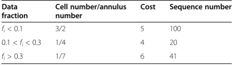
routing table. Table 2 shows an example of a routing table in SPCPM for a given node, e.g.,u. If the data frac-tion ofuis less than 0.1, between 0.1 and 0.3, and more than 0.3, the packet should be sent to a node in the third cell of annulus 2, first cell of annulus 4, and first cell of annulus 7, respectively. The cost value indicates the cost of transmitting data from the node to the SINK, and the sequence number is for the sequence number originated by the SINK node. This number is used by the DSDV al-gorithm to prevent formation of routing loops [37].
It should be noted that when a new source node with a new data flow appears in the network, the data fraction (fi) for some nodes may change. This change may cause the next hop for some nodes to alter too (see Table 2). In addition, the appearance of a new flow may activate a node previously running in the sleep mode. This reduces the cost of transmitting data for the neighboring nodes of the newly activated node. Therefore, the routing ta-bles should be updated. The transmission costs are calculated from Equation (12). In addition to the appear-ance of a new data flow, the disappearappear-ance of an existing flow may also require a route update. In such a case, the active nodes on the routing path for this flow may
switch to the sleep mode after some timeout. Another case where the routing tables should be updated is when a source node changes its data rate (significantly). This again changes the data fraction of some nodes and hence the routing tables should be updates. When the work-load of the network is dynamic, multiple rounds of route updates may be initiated at the same time, resulting in high network contention. In the DSDV technique, to re-duce the overhead of route updates in such a case, the SINK can include several default data rates in its initial route updates, based on the estimation of source rates.
In our distributed algorithm, we have assumed that ei-ther a GPS or GPS-less mechanism may be used as a localization technique to obtain the location information of the nodes. In our algorithm, we supposed that each node knew its current location relative to the SINK node. The information is used to configure the network. Due to its importance, the localization (which is not the focus of this paper) is an active area of research (see, e.g., [42-46]). For example, the techniques presented in [44-46] determine the node location based on the infor-mation of the angle of arrival between neighbor nodes. These techniques which are accurate, decentralized, and GPS-less may be the better option for being used in conjunction with SPCPM.
6.1 Performance of distributed SPCPM
In order to evaluate the performance of the distrib-uted SPCPM algorithm, we compare it with mini-mum transmission routing (MTR) [12], distributed minimum power configuration protocol (MPCP) [30], and the original DSDV [37]. A node in MTR chooses the next hop node based on minimizing the expected number of transmissions while considering the same transmission range for all the nodes. The MPCP algo-rithm is similar to the distributed SPCPM except for the fact that it does not have a cell-based configur-ation. To generate the results presented in this sec-tion, the simulator Prowler was used. Prowler is a Matlab-based network simulator that uses an event-driven structure. For the physical and MAC layer pa-rameters, we used network parameters described in [47,48]. These parameters are used for the models concerning all levels of the communication channel and application. The nondeterministic nature of the radio propagation is characterized by a probabilistic radio channel model. The radio propagation model determines the strength of a transmitted signal at a particular point of the space. The deterministic part of the propagation function can be any user-supplied function where, in this work, we used the model ex-plained in Subsection 3.2. The fading effect is also mod-eled by random disturbances. In our simulations, the required transmission power/energy for each node in an
active period is estimated based on the distance to the next hop considering the radio environment (including fading). The simulator assumed a continuous adjust-ment of the transmission power. The same assumption has been considered for implementing all other algo-rithms in this paper.
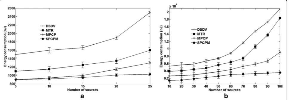
For the MAC layer, we have employed a simple CSMA/CA scheme without RTS/CTS, which is based on SMAC. Like [30], as an automatic repeat request (ARQ) mechanism, we retransmit a packet if an acknow-ledgement is not received after timer preset. The maximum number of retransmissions before dropping a packet is 4. The results were obtained for two sector-shaped configurations. In the first one, a sector-sector-shaped area withR= 400 m which was divided into 4 annuluses and 16 cells where 50 nodes were deployed. In the second configuration, the sector-shaped area had a radius of 800, 8 annuluses, 64 cells, and 200 nodes. The number of sources for these configurations changed from 5 to 25 and 10 to 100, respectively. The data packet size was 120 bytes, and the routing update packets were 40 bytes. For the energy parameters, we assumed the same values as those mentioned in section 4. The simu-lations were performed for one period of sending report by the WSN sources. It should be noted that in all simu-lations, to report the energy consumption like in Section 4, we got the sum of the average energy consumption of all network nodes. All the simulation results were ob-tained by averaging the results of ten simulation runs. We have also shown the corresponding 90% confidence interval for the results.
The energy consumptions of the protocols versus the number of sources are shown in Figure 5 which reveals that SPCPM consumes a considerably lower energy compared to those of the DSDV and MTR algorithms. This was expected because the idle power in DSDV and MTR was ignored. Note that both the SPCPM and
MPCP algorithms attempt to optimize the transmission range and the idle power. Among the two, the SPCPM method performs better. This is may be attributed to the use of the cell-based topology which provides us with the ability to use the power management technique in the node dimension. Comparing the two network config-urations indicate that as the numbers of nodes and the sources increase the efficiency of the SPCPM algorithm compared to that of MPCP improves. Also, note that the energy consumption of SPCPM slightly increases when the number of sources becomes larger than the number of cells (16 and 64, respectively). This is justified by con-sidering that in our proposed algorithm, the number of active nodes is limited by the number of cells thanks to the use of node dimension power management tech-nique (one active node in each cell). In the case of other algorithms, the energy consumptions increases more as the number of sources enlarges.
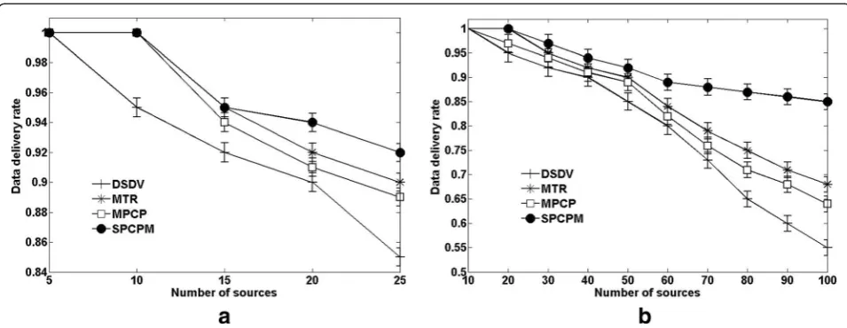
Figure 6 shows the data delivery rate of the distrib-uted algorithms at the SINK node for different algo-rithms. As the results indicate, the delivery rate of all the algorithms decreases when the number of sources increases. The SPCPM algorithm outperforms other methods due to the use of a cell-based structure which decreases the contentions during the workload increase. A comparison between the two configurations demonstrates that for DSDV, MTR, and MPCP, the increase in the number of nodes and workload lowers the delivery rate considerably. In the case of SPCPM, however, the decrease is lower. The average end-to-end delay of data packets are plotted in Figure 7, which indicates that the SPCPM algorithm leads to a higher latency compared to those of the other approaches. The reason is that SPCPM reduces the idle power by taking some nodes to the sleep state, increasing the nodes which are shared among the routes between the sources and the SINK node.
It should be mentioned that when the distributed algo-rithm is performed, the state of some nodes are changed. These changes are broadcasted in the network by the corresponding nodes via some small control messages. For this algorithm, we used the same message configur-ation as that of the MPCP algorithm. We have compared the message overheads of the algorithms in Figure 8. The results specify that the overhead of the SPCPM technique is higher. Note that the volume of the control messages is considerably smaller compared to the vol-ume of the report data, and hence, the higher overhead for the proposed algorithm should not be a major con-cern. Also, we should mention that the overheads of SPCPM and MPCP increase as the number of sources enlarges. In the case of the other two approaches, the overhead almost remain unchanged with the number of sources. This may be explained by noting that for the case of SPCPM and MPCP, before a new source starts transmitting data, its state should be changed and its routing table along with those of the neighbors should
be updated. These changes should be broadcasted for all the neighbors in the area via the control messages result-ing in increase in the message overhead for the addition of each new source.
6.2 Impact of limiting transmission power on SPCPM
The SPCPM algorithm does not assume any transmis-sion range limit (TRL). In practical cases, however, the nodes of WSN have limited transmission ranges. In this part, we study the impact of the limitation on the effi-ciency of the algorithm. It should be noted that decreas-ing the TRL of nodes lowers the efficiency of these types of algorithms. To study the effect of the TRL variation on the efficiency of the proposed algorithm, we have plotted the energy consumption of network versus the number of sources for the TRL values of 200, 400, and 800 m in the case ofR= 800 m. The decrease in the effi-ciency may be attributed to the fact that, in our algo-rithm, to lower the energy consumption, we use longer transmission ranges for small data sizes. Reducing TRL
Figure 7Average delay of a communication from source to SINK node versus number of sources.
limits the transmission ranges, which may be used for these data sizes, lowering the algorithm efficiency. For example, in Figure 9a, when the TRL value is decreased from 800 to 400 m, the transmission ranges longer than 400 m are excluded. For example, in this case, the nodes in annulus 8 cannot transmit their reports directly to the SINK node. To compare the impact of the TRL changes on the efficiencies of the algorithms, we have plotted the energy consumption of network versus the number of sources for the TRL values of 200, 400, and 800 m in the case of, for example, ψ(π/6,800 m,64,8) for both the SPCPM and MPCP algorithms. The results reveal that, on average, the amount of the energy increase with the number of sources is lower in the case of SPCPM.
6.3 Impact of assumption of equal distance hops on SPCPM
As mentioned in Subsection 5.2 A, to simplify the algo-rithm, we only considered the routes with equal distance hops to reduce the complexity (increase the speed) of the algorithm. Since some of the transmission scenarios are excluded, one may expect that the energy preservation of the algorithm is lowered. To study this, we compared the energy consumptions forψ(π/6,800 m,64,8) in the cases of including all the scenarios (complete SPCPM) and the scenarios with only (about) equal distance hops. The re-sults, which include both the TRL values of 400 and 800 m, are shown in Figure 10. As is evident from the figure, the energy preservations in these cases are not considerably different. Specifically, in the maximum case, the energy consumptions for the complete SPCPM are 4, 5, and 9% lower than those of the SPCPM in the cases of TRL = 200 m, TRL = 400 m, and TRL = 800 m, respectively. The small differences between the efficiencies of the
two algorithms may be justified by noting that the trans-mission energy constitutes a major part of the total energy consumption (the energy consumption given in Equation (7) includes both the idle as well as the trans-mission energies). As we have shown in [9], the max-imum transmission energy preservation is achieved when we consider only the scenarios which have the hops with the same distance. Also, note that changing the TRL value does not change the difference much.
6.4 Impact of SPCPM on energy hole problem
compared to those of BPC, MPCP, and MTR. Next, in Figure 11b, we have compared the normalized lifetimes of the networks with the sizes of 400, 800, and 1100 m when the SPCPM algorithm is invoked. The results sug-gest that the efficiency of the SPCPM even becomes bet-ter when the network size increases. Finally, to study the impact of the transmission range limit on the efficiency
of the algorithm in prolonging network lifetime, we have plotted the lifetimes for the TRL values of 200, 400, and 800 m in Figure 11c. Obviously, as TRL increases, there are more opportunities for skipping the nodes closer to the sink node, and hence, the longer lifetimes may be achieved. In conclusion, the SPCPM not only decreases the average energy consumption but also increases the
Figure 10Energy consumptions of the SPCPM andcomplete SPCPMalgorithms versus the number of sources forψ(π/6,800 m,64,8).(a)TRL = 200 m, (b)TRL = 400 m, and(c)TRL = 800 m.
network lifetime. Also, it should be mentioned that there are quite a number of works devoted to the energy hole problem (see, e.g.,) [9] which may be used with the SPCPM algorithm simultaneously.
7 Conclusion
In this paper, we proposed a topology control technique to reduce the energy consumption of wireless sensor networks (WSNs) based on simultaneous use of both power control and power management methods. The technique which was called SPCPM minimized the total energy consump-tion of WSNs. We discussed that none of the power control and power management approaches could optimize the energy consumptions of all the radio states. Also, it was ana-lyzed that in a sector-shaped network, the power control algorithms were effective when the traffic of the network was high while the power management algorithms were effective when traffic was low. We presented an approxima-tion algorithm with a provable performance bound and extended it to a distributed and practical algorithm. The al-gorithm dynamically updated the routes from the sources to the SINK node based on the data rates in each report period such that the energy preservation was maximized. The efficacy of the proposed algorithm was assessed by comparing its energy consumption, packet delivery rate, end-to-end delay, and control message overhead with those of the three other algorithms. The comparisons showed that the SPCPM technique conserved the energy consider-ably in both centralized and distributed forms. In addition, the packet delivery rate was higher while the end-to-end delay and control message overhead were slightly lower in the case of SPCPM.
Competing interests
The authors declare that they have no competing interests.
Acknowledgements
We would like to show our gratitude to Mehdi Kamal, Dr, University of Tehran, for sharing his pearls of wisdom with us during the course of this research.
Author details
1
Nanoelectronic Center of Excellence, School of Electrical and Computer Engineering, University of Tehran, P.O. Box 14395-515, Tehran, Iran.
2
Department of Communications and Networking, Aalto University, P.O. Box 13000, FI-00076 Espoo Aalto, Finland.
Received: 1 July 2014 Accepted: 8 April 2015
References
1. IF Akyildiz, W Su, Y Sankarasubramaniam, E Cayirci, Wireless sensor networks: a survey. J. Complex Networks.38, 393–422 (2002)
2. G Anastasi, M Conti, M Di Francesco, A Passarella, Energy conservation in wireless sensor networks: a survey. J. Ad-hoc Networks.7, 537–568 (2009) 3. DJ Cook, JC Augusto, VR Jakkula,“Ambient intelligence: technologies,
applications, and opportunities”, inPervasive and Mobile Computing, 2009, pp. 277–2985
4. DDL Mascarenas, EB Flynn, MD Todd, TG Overly, KM Farinholt, G Park, CR Farrar, Development of capacitance-based and impedance-based wireless sensors and sensor nodes for structural health monitoring applications. J. Sound Vib.329, 2410–2420 (2010)
5. E Prem, K Gilbert, B Kaliaperumal, EB Rajsingh, Research issues in wireless sensor network applications: a survey. Int. J. Inf. Electron Eng.2, 2012 (2012) 6. C Efthymiou, S Niksoletseas, J Rolim, Energy balanced data propagation in
wireless sensor networks. Wireless Networks. J12(6), 691–707 (2006) 7. J Li, P Mohapatra, Analytical modeling and mitigation techniques for the
energy hole problems in sensor networks. Pervasive Mob. Comput.3(8), 233–254 (2007)
8. M Nickray, A Afzali-kusha, R Jantti, MEA-An Energy Efficient Algorithm for dense sector based Wireless Sensor Networks. EURASIP J1, 1–13 (2012) 9. L Li, JY Halpern, P Bahl, Y Wattenhofer,“Analysis of a cone-based distributed topology control algorithm for wireless multi-hop networks”, inProceedings of the 20th Annual ACM Symposium on Principles of Distributed Computing, 2001 10. V Rodoplu, T Meng, Minimum energy mobile wireless network. IEEE J. Sel.
Areas Commun.17, 1333–1344 (1999)
11. X Wu, G Chen, SK Das, Avoiding energy holes in wireless sensor networks with nonuniform node distribution. IEEE Trans. Parallel Distrib. Syst.19, 5 (2008) 12. A Woo, T Tong, D Culler,“Taming the underlying challenges of reliable
multihop routing in sensor networks”, inProceedings of the International Conference on Embedded Networked Sensor Systems (SenSys), 2003 13. B Chen, K Jamieson, H Balakrishnan, R Morris,“Span: an energy-efficient
coordination algorithm for topology maintenance in ad hoc wireless networks,”
(ProcMobiCom 2001, Rome, Italy, 2001), pp. 70–84
14. S Narayanaswamy, V Kawadia, R Sreenivas, P Kumar,“Power control in ad hoc networks: Theory, architecture, algorithm and implementation of the COMPOW protocol,”(European Wireless Conference Next Generation Wireless Networks: Technologies, Protocols, Services and Applications, Florence, Italy, 2002), pp. 156–162
15. PR Kumar, V Kawadia,“Power control and clustering in ad hoc networks,”
16. N Li, JC Hou, L Sha,“Design and analysis of an MST-based topology control algorithm,”(Proceedings of annual joint conference of the IEEE computer and communications societies (InfoCom), Miami, 2003), pp. 1195–1206 17. M Sha, G Xing, G Zhou, S Liu, X Wang,C-MAC: Model-driven concurrent
medium access control for wireless sensor networks,”(Proc. of the 28th IEEE International Conference on Computer Communications, Rio de Janeiro, Brazil, 2009)
18. S-T Sheu, Y-Y Shih, W-T Lee, Csma/cf protocol for ieee 802.15.4 wpans. IEEE Trans. Veh. Technol.58(3), 1501–1516 (2009)
19. A Castagnetti, A Pegatoquet, T Nhan Le, M Auguin,“A joint duty-cycle and transmission power management for energy harvesting WSN”. Ieee Transactions On Industrial Informatics10, 2 (2014)
20. G Xing, C Lu, Y Zhang, Q Huang, R Pless,“Minimum power configuration in wireless sensor networks, inproceeding of the 6thACM International
Symposium on Mobile Ad Hoc Networking and Computing (MobiHoc), 2005 21. F Lavratti, AR Pinto, D Prestes, L Bolzani, F Vargas, C Montez,“A Transmission
Power Self-Optimization Technique for Wireless Sensor Networks,”Journal ISRN Communications and Networking, 2012
22. Z Zhou, S Zhou, JH Cui, S Cui, Energy-efficient cooperative communication based on power control and selective single-relay in wireless sensor networks. IEEE Trans. Wireless Commun.7(8), 3066–3079 (2008)
23. C Long, Q Zhang, B Li, HJ Yang, X Guan, Non-cooperative power control for wireless ad hoc networks with repeated games. IEEE J. Sel. Areas Commun.
25(6), 1101–1112 (2007)
24. E Tsiropoulou, G Katsinis, S Papavassiliou, Distributed uplink power control in multi-service wireless networks via a game theoretic approach with convex pricing. IEEE Trans. Parallel Distrib. Syst.23(1), 61–68 (2012)
25. W Dargie,“Dynamic Power Management in Wireless Sensor Networks: State-of-the-Art,”IEEE Sensors Journal, 2011, pp. 1518–1528
26. NA Pantazis, DD Vergados, A survey on power control issues in wireless sensor networks. Communications Surveys & Tutorials9(4), 86–107 (2007) 27. A Norouzi, A Sertbas, An integrated survey in efficient energy management
for WSN using architecture approach. Int. J. Adv. Networking Appl.03(01), 968–977 (2011)
28. G Anastasi, M Conti, MDFA Passarella, Energy conservation in wireless sensor networks: a survey. J. Ad-Hoc. Netw.7(3), 537–568 (2009) 29. Y Xu, J Heidemann, D Estrin,“Geography-informed Energy Conservation for
Ad Hoc Routing”, inProc. of ACM Mobicom, 2001
30. G Xing, C Lu, Y Zhang, Q Huang, R Pless, Minimum power configuration for wireless communication in sensor networks. ACM Trans. Sensor. Netw.3(2), 200–233 (2008)
31. Q Dong, S Banerjee, M Adler, A Misra,“Minimum energy reliable paths using unreliable wireless links”, inProc. of 6th ACM International Symposium on Mobile Ad Hoc Networking and Computing, 2005
32. M Boutabaand, L Sichitiu, Benefits of multiple battery levels for the lifetime of large wireless sensor networks. IFIP Int. Fed. Inf. Process, LNCS
3462, 1440–1444 (2005)
33. V Raghunathan, C Schurgers, S Park, MB Srivastava, Energy-aware wireless micro sensor networks. IEEE Signal Process Mag.19(2), 40–50 (2002) 34. WB Heinzelman, AP Chandrakasan, H Balakrishnan, An application-specific
protocol architecture for wireless microsensor networks. IEEE Trans. Wireless Commun.1(4), 660–670 (2002)
35. MR Garey, DS Johnson,Computers and intractability: a guide to the theory of NP-completeness, 1990(W. H. Freeman & Co, San Francisco, 1979) 36. S Singh, M Woo, SC Raghavendra,“Power-Aware routing in mobile ad hoc
networks”, In Proceedings of the 4th Annual ACM-IEEE International Conference on Mobile Computing and Networking, 1998
37. CE Perkins, P Bhagwat,Highly dynamic destination-sequenced distance-vector routing (DSDV) for mobile computers(In Proceedings of the SIGCOMM Conference on Communications Architectures, Protocols and Applications, 1994)
38. D Bertsekas, R Gallager,Data networks(Prentice-Hall, Upper Saddle River, NJ, 1987)
39. NR Paul, L Tripathy, PK Mishra, Analysis and improvement of DSDV protocol. IJCSI Int. J. Comput. Sci. Issues8(5), 1 (2011)
40. L Feeney, M Nilsson,“Investigating the energy consumption of a wireless network interface in an ad hoc networking environment”, In Proceedings of INFOCOM 2001, volume 3, pages 1548–1557(Anchorage, Alaska, 2001)
41. S PalChaudhuri,Power mode scheduling for ad hoc network routing(Master Thesis, Computer Science, Rice University, 2002)
42. N Bulushu, J Heidemann, D Estrin, GPS-less low cost outdoor localization for very small devices. IEE Pers. Commun. Mag.7(5), 28–34 (2000)
43. L Doherty, KSJ Pister, LE Ghaoui,“Convex position estimation in wireless sensor networks,”(Proceedings of the IEEE Infocom, pages: 1655-1663, Alaska, 2001) 44. R Peng,“Angle of Arrival Localization for Wireless Sensor Networks”, 3rd Annual
IEEE Communications Society on Sensor and Ad Hoc Communications and Networks, 2006
45. P Kułakowski, E Egea-López, J García-Haro, Angle-of-arrival localization based on antenna arrays for wireless sensor networks. Comput. Electrical Eng. Arch.
36(6), 1181–1186 (2010)
46. D Niculescu, B Nath,“Ad hoc positioning system (APS) using AOA”(Proc. IEEE INFOCOM 2003, San Francisco, 2003), pp. 1734–1743
47. G. Simon, Probabilistic wireless network simulator. http://www.isis.vanderbilt.edu/ projects/nest/prowler/.
48. G Simon, V Péter, M Miklós, L Ákos,“Simulation-based optimization of communication protocols for large-scale wireless sensor networks”, in
IEEEAC, paper number, 2002, p. 1136
Submit your manuscript to a
journal and benefi t from:
7 Convenient online submission
7 Rigorous peer review
7 Immediate publication on acceptance
7 Open access: articles freely available online
7 High visibility within the fi eld
7 Retaining the copyright to your article