R E S E A R C H
Open Access
An analytical model for the intercell interference
power in the downlink of wireless cellular
networks
Benoit Pijcke
1,2,3, Marie Zwingelstein-Colin
1,2,3*, Marc Gazalet
1,2,3, Mohamed Gharbi
1,2,3and Patrick Corlay
1,2,3Abstract
In this paper, we propose a methodology for estimating the statistics of the intercell interference power in the downlink of a multicellular network. We first establish an analytical expression for the probability law of the interference power when only Rayleigh multipath fading is considered. Next, focusing on a propagation
environment where small-scale Rayleigh fading as well as large-scale effects, including attenuation with distance and lognormal shadowing, are taken into consideration, we elaborate a semi-analytical method to build up the histogram of the interference power distribution. From the results obtained for this combined small- and large-scale fading context, we then develop a statistical model for the interference power distribution. The interest of this model lies in the fact that it can be applied to a large range of values of the shadowing parameter. The proposed methods can also be easily extended to other types of networks.
Keywords:Intercell interference power, Statistical modeling, Wireless networks, Rayleigh fading, lognormal shadowing
I Introduction
In the emerging wireless communication standards LTE-Advanced and Mobile WiMAX, aggressive spectrum reuse is mandatory in order to achieve the increased spectral efficiency required by IMT-Advanced for the 4th generation of standard telephony. However, since spectrum reuse comes at the expense of increased cell interference, these standards explicitly require inter-ference management as a basic system functionality [1-3]. The research area related to the development and analysis of interference management techniques, mostly in relation with the more general subject of radio resource management, is very dynamic, as witnessed by the high number of relevant recent contributions in this area [4-10]. All these new standards use OFDMA as the modulation and the multiple access scheme. In an OFDMA system, there is no intracell interference as the users remain orthogonal, even through multipath chan-nels. However, when users from different cells are pre-sent at the same time on the same subchannel, which is
the case under aggressive frequency reuse, signals super-pose, leading to some form of intercell interference.
Providing statistical models of the interference power is essential to allow for an accurate evaluation of net-work performances without the need for lengthy and costly Monte Carlo simulations. The statistical charac-terization of the interferences has been investigated for a long time, under lots of different scenarios, and fol-lowing several approaches. The distribution of cumu-lated instantaneous interference power in a Rayleigh fading channel was investigated in [11], where an infi-nite number of interfering stations was considered. In [12], the interference power statistics is obtained analyti-cally for the uplink and downlink of a cellular system, but in the presence of large-scale fading only. Interfer-ence modeling when considering only large-scale fading effects has also been investigated in [13-15], where the emphasis is on finding a good approximation of the log-normal sum distribution. In [16], an analytical derivation of the probability density function (pdf) of the adjacent channel interference is derived for the uplink. More recently, in [17], the pdf of the downlink SINR was derived in the context of randomly located femtocells * Correspondence: [email protected]
1Université Lille Nord de France, 59000 Lille, France
Full list of author information is available at the end of the article
via a semi-analytical method. Other contributions have focused directly on the analysis of a particular perfor-mance measure that is influenced by intercell interfer-ence, like the probability of outage and the radio spectrum efficiency [18-20]. The analysis of interference in dense asynchronous networks, such as ad hoc net-works, is also an active research area, for which a deep review of the recent developments can be found in [21,22].
In this paper, we derive a semi-analytical methodol-ogy to estimate the statistics of the intercell interfer-ence power in a wireless cellular network, when the combined effects of large-scale and small-scale multi-path fading are taken into consideration. Large-scale effects include attenuation with distance (path loss) as well as lognormal shadowing, and the small-scale fad-ing is Rayleigh distributed. We consider a distributed wireless multicellular network, in both cases where power control and no power control are applied. The proposed methodology is semi-analytical, in that the statistical estimate of the interference power resulting fromN> 1 interferers is obtained by numerical techni-ques from an analytically derived interference model for one interferer. The methodology is valid in a quite general framework; we have chosen to present it using a hexagonal network layout, although it can handle any other topology. We validate the proposed methods by comparing the moments of the estimates to the exact moments of the distribution which can be derived analytically. Using this methodology, we are able to provide a very good estimate of the pdf of the interference power, for different values of the shadow-ing standard deviation, sdB. Based on these estimates, we then propose an analytical statistical model of the interference power, based on a modified Burr distribu-tion, which includes five parameters. This analytical, parameterized by sdB, model will hopefully serve as a practical tool for the assessment and simulation of wireless cellular networks when the effect of shadow-ing is to be considered.
The main contributions of this paper are as follows:
• In the special situation where only path loss and Rayleigh fading are considered (no shadowing), we derive a very accurate approximated analytical expression for the pdf and the cumulative distribu-tion funcdistribu-tion (cdf) of the intercell interference power;
•We propose a semi-analytical method for the esti-mation of the pdf of the intercell interference power in a multicellular network when the combined pro-pagation effects of path loss, Rayleigh fading and lognor-mal shadowing are considered;
• Based on this method, we derive an analytical
model for the pdf of the intercell interference power by slightly modifying a Burr probability distribution. This model is parameterized by the lognormal stan-dard deviation sdB, and its interest resides in the fact that it is valid on the whole [0, 12]-dB range of values.
The remainder of this paper is organized as follows. In Section II, we describe the multicell downlink trans-mission environment, and we provide the expression of the interference power for which we want to find a statistical model. In Section III, the original methodol-ogy for estimating the statistics of the interference power is presented. For this purpose, we examine in Section III-A the particular case where path loss and Rayleigh fast-fading are the only fading phenomena considered. In Section III-B, we include the shadowing effect and we consider in the first instance the contri-bution of one interfering cell. We then generalize toN >1 interferers. In Section IV, we apply the proposed method to estimate the pdf of the interference power in a typical multicellular network, under two frequency reuse scenarios. Section V is dedicated to the para-metric analytical modeling of the interference power. Section VI concludes the paper by summarizing the
proposed methods and by presenting some
perspectives.
We will use the following notation for the rest of the paper. Non-bold letters such as x are used to denote scalar variables, and |x| is the magnitude ofx. Bold let-ters like x denote vectors. We useE{X}to denote the expectation ofX. The pdf and cdf of the random vari-able (r.v.) X will be denoted as pX (x) and FX (x), respectively.
II Multicell downlink transmission model
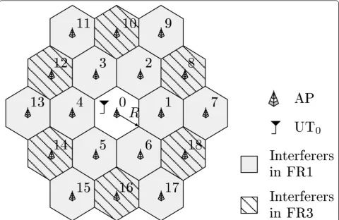
consider UT in cell 0 (denoted UT0, see Figure 1), for it is surrounded by 18 potential interferers. For UT0, the received signal on OFDMA subchannelℓ at time slotm can be modeled as
y0(m,) =h0(m,)x0(m,) + N
n=1
hn(m,)xn(m,) +w(m,).
Here, x0 (m, ℓ) represents the information symbol intended to UT0and xn(m,ℓ),n≠0, thenth interfering symbol (this symbol is sent from AP nto its respective user). The coefficient hn (m, ℓ) denotes the instanta-neous gain of theℓth (interfering) subchannel from AP nto UT0. Each subchannelℓ is subject to additive white Gaussian noisew(m, ℓ). In the following, we will focus without loss of generality on a single OFDMA subchan-nel, thereby omitting subchannel index ℓ in all subse-quent notations.
Two frequency reuse scenarios will be considered (see Figure 1):
• the full frequency reuse pattern, denoted FR1,
where all APs in the network transmit at the same
time using the same frequency range (N= 18 inter-cell interferers);
•a partial frequency reuse pattern, denoted FR3, with reuse factor 3 (N= 6 interferers).
Each channel is assumed to be flat-fading, possibly experiencing small-scale multipath fading and/or large-scale effects. For the rest of the paper, we concentrate on the instantaneouschannel power gainaGn(rn), which is proportional to |hn(m)|2 and can be expressed as a three-factor product:
Gn(rn)=Gpl,n(rn)Gf,nGs,n,n= 1, 2,. . .,N. (1)
In the above equation, rn denotes the distance
between UT0 and AP n(distances rn are functions of UT0’s position within its cell). Gpl,n(rn) =K(1/rn)g is the (deterministic) path loss (normalized with distance, see Appendix A), where Kis a constant, and g repre-sents the path loss exponent. The Rayleigh fading gain Gf,nis modeled by an exponential distribution with rate parameter equal to 1, i.e.,EGf,n
= 1; we denote the corresponding pdf by pGf,n(x). The shadowing gain Gs,n
is modeled by a lognormal distribution whose pdf can
whereξ = 10/ln(10) [23]. Note that the importance of the shadowing phenomenon is directly related to the standard deviationsdB. For a givensdB, the parameter
μdB is determined to ensure a unit mean shadowing
gain:EGs,n
nth interfering channel’s Rayleigh fading and shadowing components cause the actual gain Gn (rn) to fluctuate about its mean valueGpl,n(rn).
The total interference power undergone by UT0
can then be written as I= N lows, we consider that all APs transmit at the same power, i.e.,Pn=Pfor alln. This corresponds to, e.g., a fast-fading environment where no channel state information feeds back from mobile users to APs, which results in a no power control scheme where all APs transmit at the maxi-mum power; although crude, this scheme can be seen as a lower bound on performance for real systems. Considering that each AP transmits at the same powerPalso applies to a more practical scenario where APs have access to chan-nel state information, and power control is associated with the opportunistic scheduling policy proposed (and proved to be sum-rate optimal) in [10], when the number of users per cell is high (since in this case, it can be expected that the channels between users scheduled at the same time and their serving APs have about the same power gains).
Thus, the interference simplifies toI=P N
n=1Gn(rn).
We now define the interference gain-which will be
denotedG-as being the sum of the channel power gains between the interested user and theNinterferers, i.e.,
G=
(Note that Gis a function of UT0’s location through the distancesrn.) So, asI=PG, characterizing the inter-ference power Iis equivalent to studying the interfer-ence gainG. We will concentrate on the latter in the subsequent sections.
III Methodology
We are now interested in finding an estimate of the pdf of the random interference gain (2). Since direct calculation of the pdf does not seem possible, we aim
at producing an accurate histogram for the interfer-ence gain Gthat will then be modeled using a speci-fied statistical distribution. Such a histogram is constructed from a set of samples called a typical set, i.e., a discrete ensemble of values that accurately repre-sents a random phenomenon. Traditionally (and espe-cially in the telecommunications area), this typical set is issued from Monte Carlo simulations, which might, at first sight, produce satisfying results. However, in a propagation environment that is subject to intense sha-dowing (i.e., for large values of the [0, 12]-dB range under consideration), the classical Monte Carlo method fails at producing a representative set of sampled gains [24,25]. This can be explained by exam-ining the particular distribution involved, for one sin-gle as well as for multiple interfering cells. A typical cdf of the interference gain (single or multiple inter-ferers) for a high value of sdB belongs to the class of heavy-tailed distributions [26], for which the least-frequently occurring values-also called rare events-are the most important ones, as a proportion of the total population, in terms of moments. A finite-time random drawing process performed on this cdf never produces these rare events because of their very low probabilities, which causes the resulting set to be not typical. Hence, the need for a new approach.
As will be seen in Subsection B, the pdf and the cdf of the interference gain for one single interferer may be expressed in its integral form. From this expression, we propose the following two-step approach:
1. Produce a typical set of gains for one interferer using the generalized inverse method. This method con-sists in generating a typical set of samples corresponding to an arbitrary continuous cdfFand is based upon the following property: ifUis a uniform [0, 1] r.v., then F-1 (U) has cdfF;
2. Produce a typical set for multiple interferers by ade-quately combining typical sets from single interferers and the Monte Carlo computational technique.
A Special case: no shadowing
We start this section by considering a propagation environment in which the only fading phenomenon is due to Rayleigh multipath fading. In this particular case, (1) simplifies to
Gn(rn)=Gpl,n(rn)Gf,n. (3)
We now introduce an original approximation that will help simplify further computations. We can see that in (3), it is UT0’s random position that makes the path loss Gpl,n (rn) fluctuate, when the randomness ofGf,nis due to Rayleigh fading. But, it is worth noting that, although both phenomena are random, path loss fluctuations dif-fer from multipath fading in an important way: the path loss takes values in a finite set (related to UT0’s location within its cell), whereas the variations due to fading have an (theoretically) infinite dynamic range. Since path loss fluctuations’ dynamics are very small com-pared to fading’s, we propose to approximate (3) by replacing each gainGpl,n(rn) by its average value, which leads to
Gn≈E rn
Gpl,n(rn)
Gf,n
= E
r0,θ
Gpl,n
fn(r0,θ)
Gf,n,
(4)
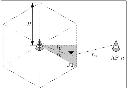
using the notationrn=fn (r0,θ), n= 1, 2,...,N, where (r0,θ) are UT0’s polar coordinates, as depicted in Figure
2. By examining (4), we see that, under this approxima-tion, Gn does not depend on UT0’s varying position anymore.
We further note that Gn, as expressed in (4), is an exponentially distributed r.v. with rate parameter 1/ln [27], ln-which we call the average path loss-being defined as follows:
λn= E
r0,θ
Gpl,n
fn(r0,θ)
. (5)
Using (5), (4) can also be written as
Gn≈λnGf,n, (6)
and the intercell interference gain (2) can be reduced to a sum of independent (but not identically distributed) exponential r.v.’s:
G≈ N
n=1
λnGf,n. (7)
G, as expressed in (7), is a r.v. whose cdf, denotedFG (g), has a closed form expression available in the litera-ture [28]; it can be expressed as
FG(x)= 1−
The pdf, denoted pG (g), can be easily calculated by deriving (8):
In Section IV-A, it is first shown that approximation (4) is valid in the case of one single interfering cell. This consequently validates the proposed model (7) in the case of multiple interfering cells, which we show for both frequency reuse patterns FR1 and FR3.
B General case: attenuation with distance, shadowing and multipath fading
Let us now focus on characterizing the distribution of the intercell interference gainGin a propagation envir-onment where Rayleigh fading as well as shadowing (due to obstacles between the transmitter and receiver that attenuate signal power) are taken into account. To the best of our knowledge, no closed form expression for the interference gain Gexists in the literature. But, as will be seen in Section III-B.2, we determine an ana-lytical formula (under integral form) of the distribution of the interference gain for one interferer. Using this result, we are able to obtain a histogram for G’s distri-bution in the presence of multiple interferers.
For this purpose, we proceed in two steps: first, we compute a typical set for the interference gain pro-duced by one single interferer. As described in Section III-B.2, this is done by numerical computation (from the integral-form cdf), followed by non-uniform parti-tioning, and then inversion, of the cdf. Then, we
gen-erate a typical set for N interferers using an
appropriate combination of the (weighted byln) typi-cal sets of each single interferer (Section III-B.3). The accuracy of the proposed method will be evaluated in both single- and multiple-interferer cases by compar-ing the actual moments computed from the typical sets with the exact moments of the interference gain distribution (which can be formulated analytically, as will be seen in Section III-B.1).
1) Preliminaries: We begin this section by examining two important points.
When taking into account multipath fading as well as shadowing as the fading effects in the propagation environment, a question arises about the validity of the original approximation (6). Fortunately, our approxi-mation is being strengthened by this additional contri-bution due to shadowing, since this phenomenon is just another source of infinite-dynamics randomness. Taking shadowing into consideration amounts to introducing an additional term in (6) that can now be written as
Gn≈λnGf,nGs,n. (10)
A second point pertains to the moments of both statistical distributions of Gn (single interferer) andG (multiple interferers). Using approximation (10), it is
shown in Appendix B that the kth-order moment of
Gn’s distribution has the following expression:
E(Gn)k
Computation of thekth-order moment ofG’s distribu-tion is done in Appendix C and leads to the following formula:
an N -dimensional vector whose sum of components
is written|a| =Nn=1αn, andλa=λα11λα
2
2 . . . λα
N
N. So, the
summation in Equation (12) is taken over all sequences of non-negative integer indicesa1throughaNsuch that the sum of allanisk. Note that the 1st-order moment,
is a quantity of particular interest because it is propor-tional to theaveragepower of the interference signal.
As closed form expressions of moments have been determined, they may be used in evaluating the accuracy of typical sets for both single- and multiple-interferer statistical laws.
2) Single interferer:We now turn on to computing a typical set for the interference gain produced by one interferer. For convenience, the average path loss (5) for this single interferer is normalized to 1, i.e.,ln= 1, so (10) reduces to
AsGnis the product of two independent r.v.’s, its cdf can be written as
FGn(x)= Recalling that Gs,n is modeled as a lognormal r.v., we have, using the same notations as in Section II,
FGs,n
plementary error function of Gaussian statistics. Repla-cingpGf,n(u)andFGs,n
x/uby their respective expression in (15), we obtain an integral-form expression for the cdf of the intercell interference gain produced by one single interferer:
We are now interested in generating a typical set of the interference gain Gn; we denote this typical set by S
n, where ℓis the number of elements in the set. It was
mentioned in Section III that, though widely used in tel-ecommunications, the Monte Carlo computational tech-nique proves inefficient for large values of sdB. An interesting alternative method is the generalized inverse method, for which anℓ-element typical set for a given distribution is obtained by anℓ-level uniform partition-ing, followed by inversion, of the cdf. Now, we know that, for large values ofsdB, the distribution ofGn exhi-bits the heavy-tailed property, which means, as described before, that the least frequently occurring values (i.e., the highest gains) are the most important ones in terms of moments. Therefore, taking these high-est amplitudes into consideration using the ‘classical’ generalized inverse method would require a finer parti-tioning of the cdf, which would produce a typical set made up of a huge amount of elements.
In order to construct a typical set with a reasonable
value for ℓ, we propose to accommodate the
above-mentioned method by performing a non-uniform
parti-tioning ofGn’s cdf, and, as high amplitudes are impor-tant in terms of moments, we proceed with a finer
partitioning of the [0, 1] segment for values close to 1. The implementation details of the method are described on Figure 3; they result from a good compromise between accuracy and simplicity. We first divide the interval [0 1] of the cdf intoJ intervals, numbered j= 1,...,J, of different lengths: thejth interval has length dj = 9 × 10-j, j = 1,..., J - 1; and the last interval has
lengthdj= 10-J to ensure
J
j=1δj= 1. We next perform
a P -level uniform partitioning on each interval, i.e., each interval is now partitioned by P equally spaced points. Finally, we invert the partitioned cdf to obtain a typical set Snof cardinality ℓ = J × P. Also, as the proposed partitioning is non-uniform, Snneeds to be associated a probability set: the probability of an ele-ment computed from thejth interval is δj =dj/P. It can be shown (see Section IV-B) that usingJ = 25 intervals
containing P = 900 points each-which results in a
typical set that contains onlyℓ = 25 × 900 = 22,500
ele-mentsb-guarantees that up to third-order moments
derived from the typical set are within 1% of the exact values for allsdB’s.
3) Multiple interferers: We now focus on finding an L-element typical set-denotedSL-for the interference gain Gthat must be computed from Ntypical setsSn, n= 1,2,...,N.
We first note that interferer n’s typical set can be directly obtained by weighting each element ofSnby its average path lossln; we will denote interferern’s typical set by λnSn. Let us now find a way to produce the
ensembleSLfrom the typical setsλnSn.
Ideally,SLshould be constructed by considering all combinations of the elements of the typical sets λnSn,
but the cardinality of the resulting set, L=N=(JP)N,
would rapidly become prohibitive as the numberN of
interferers increases.
To get rid of this complexity, we point out that the above-mentioned ideal (exhaustive) solution can also be viewed as an exhaustive combination of intervals (JN combinations) associated with an exhaustive combina-tion of elements within each interval combinacombina-tion (PN combinations). And, we observe that the most impor-tant part of this exhaustive solution pertains to the combination of intervals, i.e., the combination of ele-ments belonging to interval j of typical setλnSnwith
elements belonging to interval k, k ≠ j typical set
λmSm,m=n. So, a way to construct a (near-optimal)
following procedure: for each of theJNcombinations of NP-point intervals,
• Perform a random permutation of thePelements
within each of theNP-point intervalsc;
• Add up these N permuted P-point intervals to
obtain one resulting P-element interval.
This lastP-element interval approximates thePN -ele-ment interval that would have resulted from an exhaus-tive combination of elements within the considered interval combination. Now, as there areJNinterval com-binations, the resulting typical set would contain JNP elements, which can still be prohibitive, so this second solution-which we will refer to as thenear-optimal solu-tion-can not be applied as such.
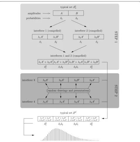
We eventually propose a novel approach which makes use of this near-optimal solution and is based on the following two-step algorithm:
Step 1 Apply exhaustive combinations of intervals to a subset ofMinterfering links;
Step 2 Perform Monte Carlo simulations for theN -Mremaining links.
We now detail the principle of the proposed method. In Step 1, we apply the near-optimal solution described previously, but to a subset of M < N interfering links
which we will callcompelledlinks. The compelled links are chosen to have the highest average path losses (l1 ≥ ... lM ≥... lN) so as to minimize errors in other (non-compelled) interfering links. The exhaustive combina-tion of the J intervals for M compelled links obtained from the near-optimal solution thus results inoneset of JM
Pelements. In Step 2, we build up aJMP-element set foreach of the N- Mremaining, non-compelled, links by performing JMrandom drawings of intervals accord-ing to the probability set {δj}, j = 1, 2,..., J. As in the near-optimal solution, a random permutation of the ele-ments is applied at each drawing. The ensemble of amplitudes of the intercell interference gain G-the so-called typical set SL-is then constructed by adding up theseN- M + 1 sets; it is of cardinalityL=JMP. Asso-ciated to SLis a probability set determined as follows: to each interval is associated a weightwhich is the pro-duct of probabilities δk of intervals issued from com-pelled links (for non-comcom-pelled links, probabilities are accounted for by means of the random selection pro-cess); these weights are then normalized to obtain prob-abilities. Finally, the histogram of the interference gain
G can be constructed from these resulting amplitude
and probability sets. It is important to note, however, that, as a random drawing process is involved, a number of iterations might be needed in order for this process
to converge (elements of SLand associated probabilities are averaged at each iteration). We will call this
semi-analytical technique the Monte Carlo-panel method
(MCP, in short)d.
The MCP method is illustrated on Figure 4 forN= 4 interfering cells,M = 2 compelled links andJ= 2 inter-vals per typical set (these interinter-vals-denotedA and B -have probabilitiesδ1 = 0.9 andδ2= 0.1, respectively, and each one of them contains P elements). Step 1 of the algorithm is summarized in the light gray-shaded box:
intervals from typical setsS1andS2(corresponding to compelled interfering links 1 and 2 and weighted by their respective average path lossesl1 andl2) are com-bined together, as described in the near-optimal solu-tion, to obtain a set of amplitudes of cardinality 4P representative of the two compelled links; associated to this set of amplitudes is a set of weights {0.81, 0.09, 0.09, 0.01}. The dark gray-shaded box summarizes Step 2: for each non-compelled interfering link, a 4P-element set of amplitudes is made up by four intervals (Aor B)
Figure 4Illustration of the MCP method forN= 4 interfering cells,M= 2 compelled links andJ= 2 intervals per link (denotedAand
drawn according to the probability set {0.9, 0.1} and applied random permutations. The typical set SL(with
L= 4P in our example) is then obtained by summing
up together all these sets. The histogram of the interfer-ence gain Gis constructed fromS4Pand the associated
probability sete. Note that one random permutation of the interval (permuted intervals have been assigned the prime symbol) is performed at each(compelled or ran-dom) manipulation of an interval.
Implementing the MCP method, however, requires cautiousness. In non-compelled links, random draw-ings of intervals are performed based on the probabil-ity set {δj}, j = 1, 2,..., J. In this process, lowest-probability intervals, which contain the highest inter-ference gains, are totally ignored for two reasons. The first reason pertains to the fact that obtaining a signifi-cant frequency of appearance of such rare events would require a prohibitive number of simulation runs. The second reason is due to limitations inherent to software simulation tools which use pseudo-random number generators to generate sequences of ‘random’ numbers belonging to a fixed set of values. In order to take into account the ignorance of the contribution of the highest interference gains of the N- M non-com-pelled interfering links in the probability set {δj}, we suggest the following work around: in these links, we intentionally make exclusive use of theJ,1≤J <J, first intervals, and we associate them a loaded prob-ability setδj
the particular non-uniform partitioning described pre-viously, we have:α= 1/1−0.1J1.
Now, as was mentioned before, high amplitudes play an important role in terms of moments. Although the impact of neglecting them in non-compelled links is globally limited because these links are weighted by smaller average path losses ln(n=M +1,...,N), it has to be compensated in order to satisfy the 1st-order moment constraint (i.e., the sampled mean has to con-verge to the exact valuef). For this purpose, small (resp. large) amplitudes need to be underweighted (resp. over-weighted). Thus, an underweighting multiplicative fac-tor, denoted f-, is applied to amplitudes of theJ first intervals of compelled links; similarly, an overweighting multiplicative factor f+ is applied to amplitudes of the
lastN−J intervals. (Computation details of factorsf -andf+ are given in Appendix D.)
Let us last notice that the choice for values ofM and J is a trade-off between different aspects: cardinality of the resulting typical set (i.e., tractable number of points), number of simulation runs and accuracy of the
histo-gram. We have determined that M= 2 andJ = 3meet
all these requirements.
IV Numerical results
In this section, we present numerical results related to the different methods introduced in the preceding sec-tion. In Section IV-A, we first examine the validity of the original approximation introduced in Section III, stating that the interference gainGn(and, consequently, G) does not depend on the user’s position within its cell. For this purpose, we compare the approximation of Ggiven by (6) with the‘exact’formula (3). Then, in Sec-tion IV-B, we obtain the histogram of the interference gainGn(one single interferer) by applying the non-uni-form partitioning generalized inverse method described in III-B.2. Finally, the MCP method (see III-B.3) is used to build up the histogram of the interference gain for multiple interferers in Section IV-C.
We use the following simulation parameters. We con-sider a system functioning at 1 GHz. We fix the cell radius toR= 700 m,d0= 10 m, and the path loss expo-nent to 3.2, which corresponds to a typical urban envir-onment, as described in the COST-231 reference model [29]. The reference distance is chosen to be equal to 2R. Average path losses ln, n = 1, 2,..., N, are determined numerically using (5) and are summarized in Table 1.
A No shadowing
In this section, we evaluate the proposed approximation (6) against Monte Carlo simulations performed on (3). We first consider the contribution of one interfering cell, and in this regard, we examine two opposite sce-narios: one for which the investigated interferer (i.e., AP 1) produces the largest dynamic range for the intercell interference power undergone by a user in the gray-shaded triangular area of Figure 2; the other one for which the investigated cell (i.e., AP 13) has the smallest dynamics. Obviously, both dynamics differently impact the accuracy of our model. Note that, in both cases, the sum of interference gains (7) reduces to one exponential r.v. Modeled and simulated pdf’s for above-mentioned scenarios are plotted in Figures 5 and 6, respectively, and the good match of the curves shows that the pro-posed method is a good approximation.
probability laws (2) and (7), respectively, closely match for both frequency reuse patterns. We also note that simulated and approximated curves are closer to one another for FR3 than they are for FR1. As explained before for the single-interferer scenario, fluctuations of actual path losses Gpl,n (rn), n = 7,..., 18, can be assumed to have about the same dynamic range, but these dynamics are smaller than those of gainsGpl,n(rn), n= 1,..., 6.
B Shadowing, one interferer
In this section, we make use of the non-uniform parti-tioning generalized inversion method introduced in Sec-tion III-B.2 to obtain a typical set for the interference gain of one interferer. Table 2 presents the three first moments computed from typical set Sn, as compared with the exact moments of the distribution of the inter-ference gainGn. We see that moments issued from the typical set are far beyond the 1% accuracy requirement. The proposed method also outperforms the Monte Carlo simulation technique, which cannot be guaranteed to converge for such a small number of points.
Histograms of the interference gain Gn computed
from typical setSnis illustrated on Figure 9 for different values ofsdB.
C Shadowing, multiple interferers
We now evaluate the MCP method developed in Section III-B.3. We have determined that 20,000 iterations of the base MCP algorithm guarantee that the 1st-order moment computed from any typical set (whateversdBvalue is con-sidered) converges to its exact value (13). Table 2 presents
Figure 5 Simulated versus modeled pdf of the intercell interference power with no shadowing when AP 1 is the only interferer. Since AP 1 produces the largest dynamics for the interference power undergone by a user in thegray-shadedsector of Fig. 2 with only one interfering cell, these curves correspond to the worst-case scenario for validating our approximation.
Table 1 Average path lossesln,n= 1, 2,...,N, defined by (6), in decreasing order of importance
FR1 (N= 18) FR3 (N= 6)
N ln APm n ln APm
1 6.467 1 1 0.568 8
2 3.588 2 2 0.426 18
3 1.708 6 3 0.307 10
4 1.069 3 4 0.219 16
5 0.767 5 5 0.178 12
6 0.663 4 6 0.158 14
7 0.568 8
8 0.426 18
9 0.316 7
10 0.307 10
11 0.260 9
12 0.219 16
13 0.188 17
14 0.178 12
15 0.158 14
16 0.145 11
17 0.118 15
18 0.107 13
Each indexmof column APmcorresponds to index of average path lossln(n ≠m, in general)
Figure 7 Simulated versus modeled pdf of the intercell interference powerGfor frequency reuse pattern FR1. Figure 6 Simulated versus modeled pdf of the intercell interference power with no shadowing when AP 13 is the only interferer. AP 13 produces the smallest dynamics for the
the values of the 1st-order moment ofG, both exact (ana-lytical) and approximated (computed from the typical set). We can see that the proposed method performs very well for the whole range ofsdBvalues.
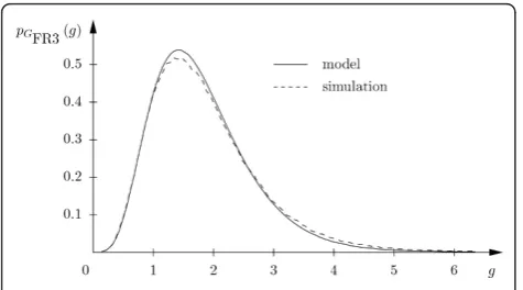
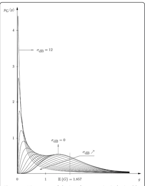
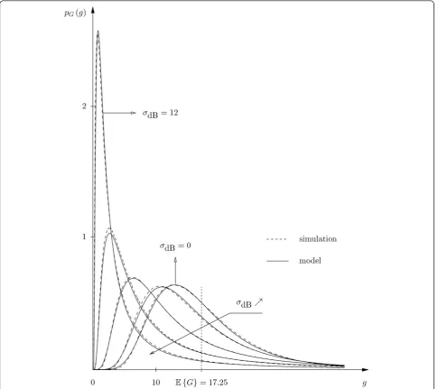
Histograms of the interference gain Gcomputed from typical sets obtained by the MCP method are illustrated on Figure 10 (FR1 scenario) and Figure 11 (FR3 sce-nario) for different values ofsdB.
V Statistical model
In Section III, we developed analytical and numerical methods to build up a good approximation of the histo-gram of the interference gainG. In this section, we aim at using this result to elaborate a statistical model forG, i.e., a closed form expression of the probability law,
characterized by the shadowing parameter sdB. This
task is challenging in that one single parametric law is required, that is valid for propagation environments which considerably vary depending upon the shadowing phenomenon (parameter sdB), and that is applicable to various frequency reuse scenarios (FR1 and FR3).
We initialize the modeling process by extracting useful information from a careful analysis of the histograms of the interference gainG(see Figures 10, 11). We first note thatGis a positive continuous r.v. We then observe that all curves are asymmetric, and this property is even more pronounced for large values ofsdB. In this case, G’s pdf’s also have a sharper peak and a longer, fatter tail, the last of
Figure 8 Simulated versus modeled pdf of the intercell interference powerGfor frequency reuse pattern FR3.
Table 2 Exact and approximated moments for one single interferer and for multiple interferers
No shadowing (sdB= 0 dB)
Intense shadowing (sdB= 12 dB)
Exact Approximated Exact Approximated
E{(Gn)} 1 1 1 0.990
E(Gn)2
2 2 4.138 · 103 1.119 · 103 E(Gn)3
6 6 53.127 · 109 13.246 · 106 E{(G)}(FR1) 17.25 17.10 17.25 17.08 E{(G)}(FR3) 1.857 1.857 1.857 1.855
Figure 9 Histograms of the interference gain Gn (one
interferer) for different values ofsdB.
which being a characteristic of heavy-tailed distributions (a.k.a.power distributions), as already mentioned.
Due to the strongly skewed nature of the interference gain distribution for largesdB’s, a power-type statistical model turns out to be suitable here.
In this regard, a Pareto-like distribution seems to be a good candidate, so we focus, in first approximation, on a 3-parameter Burr-type xii distribution [27]. The Burr distribution has a flexible shape and controllable loca-tion and scale, which makes it appealing to fit any given set of unimodal data that exhibit a heavy-tail behavior (e.g., it is an appropriate model for characterizing insur-ance claim sizes). However, as three parameters seem to not be sufficient to correctly characterize the interfer-ence gain distribution under those particularly tight con-straints, another law is required, which offers greater flexibility to match the whole range ofsdBvalues. Such
a flexibility is provided by introducing an additional shape parameter into the Burr distribution, based on the following property [30]: ifF(x) is a cdf, so is (F(x))h,∀h
>0. Thus, we have established a new Burr-based prob-ability law, whose cdf-denotedFG(x)-is given by
FG(x)= the scale parameter of the distribution. G’s pdf-denoted pG(x)-can be easily obtained by deriving (19):
pG(x)= ηα
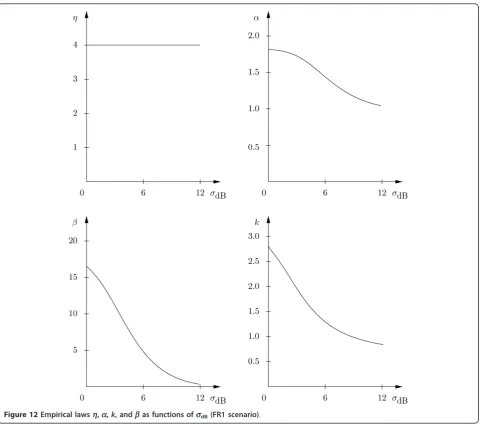
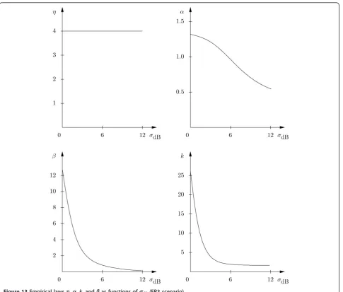
We next establish a parametric family of functions (parameterized bysdB) for the interference gainGby determining empirical formulas for parametersh, a, k, andb. For this purpose, we propose that all parameters (whatever frequency scenario is considered) be modeled by the same 6-parameter functionfthat has the follow-ing expression:
determined empirically and are summarized in Table 3. Corresponding empirical lawsf, as functions ofsdB, are plotted on Figures 12 (FR1 scenario) and 13 (FR3 scenario). The pdf’s of the proposed statistical model are superimposed on histograms obtained by the MCP method for different values of the shadowing parameter
sdB on Figure 14 (resp. Figure 15) for the FR1 (resp. FR3) scenario. We now come to the last step of our modeling process. As seen earlier, MCP-obtained histo-grams and the proposed Burr-based distributions closely match for the whole range ofsdB. However, care must be taken in defining the range of gains for which our model is valid. And indeed, the Burr-based statistical law needs to be truncated at a maximum value-denoted
Figure 11Histograms of the interference gainGobtained by the MCP method (FR3 scenario).
xt-defined in such a way that the 1st-order moment constraint holds, which we can write
xt
0
xpG(x)dx=E{G},
whereE{G}is the exact mean (13). As a consequence of this truncation process, a normalizing factor,
A= 1
1−P(x>xt)
, (22)
has to be incorporated in both the cdf and pdf of the elaborated model, which are then written AFG(x) and ApG(x), respectively. Regarding the empirical lawxtas a function ofsdB, we also propose the same 5-parameter function for both FR1 and FR3 scenarios:
xt(σdB)=a1·exp
σdB a2
a3 · exp
exp
−
σdB−a4 a5
2
, (23)
where coefficients ai, i = 1, 2,..., 6 have been deter-mined empirically and are summarized in Table 4. Empirical laws xt, as functions of sdB, are plotted on Figures 16 (FR1 scenario) and 17 (FR3 scenario). The normalizing factor may be easily computed by replacing xtby its actual value in (22).
VI Conclusion and future work
In this paper, we have proposed a methodology to esti-mate the statistics of the intercell interference power in the downlink of a multicellular network. In a propaga-tion environment subject only to path loss and multi-path Rayleigh fading, we have established an accurate
approximated analytical expression for the interference power distribution. Then, considering the combined effects of path loss, lognormal shadowing and Rayleigh fading, we have proposed a semi-analytical method for the estimation of the pdf of the interference power. Finally, we have developed a statistical model
parameter-ized by the shadowing parameter sdB and valid on a
large range of values ([0, 12] dB). It is our hope that the methods described in this paper are sufficiently detailed to enable the reader to apply them to other types of environments.
A future work will pertain to improving the statistical interference power model by more closely linking the proposed model developed for a combined Rayleigh fad-ing-lognormal shadowing environment to the ‘exact’ analytical formula obtained in the case where only Ray-leigh fading was considered. Another perspective is to
apply the proposed methods to other wireless network topologies (e.g., ad hoc networks,...).
Appendix
A Normalized channel power gain
In this paper, we concentrate on thechannel power gain Hn (rn) = |hn(m)|2, wherehn (m) is the instantaneous gain of the channel between APnand UT0.Hn(rn) can be expressed as a three-factor product:
Hn(rn)=Hpl,n(rn)Gf,nGs,n, (24)
wherernrepresents the distance between UT0 and AP n(distances rnare functions of UT0’s position within its cell), andHpl,n(rn),Gf,nandGs,nrepresent the path loss, multipath Rayleigh fading and shadowing components, respectively. We now further describe these last three components.
The (deterministic) path lossHpl,n (rn) diminishes as the distancernbetween UT0 and APnincreases, based on the common power law [23]
Hpl,n(rn)=K
d0
rn γ
, (25)
where K= (c/(4πfd0))2 is a dimensionless constant, with c being the speed of light, f, the operating fre-quency, andd0, a reference distance for the antenna far-field; andgrepresents the path loss exponent. In order to make our study independent from the antenna char-acteristics and the cell size, we rewrite (25) under the following form:
Hpl,n(rn)=K
d0
dref
γ dref
rn γ
, (26)
where dref is a reference distance, and we introduce thenormalized path loss Gpl,n(rn), defined as follows:
Gpl,n(rn)=
dref
rn γ
. (27)
From (26) and (27), we establish the following rela-tionship:
Gpl,n(rn)=
1
K
d0 dref
In a similar manner, we define thenormalized instan-taneous power gain Gn(rn) as follows:
Gn(rn)=
1
Kd0 dref
γHn(rn)
=Gpl,n(rn)Gf,nGs,n,
(29)
where (29) derives from (24) and (28).
B Computation of moments for one interferer
We find the closed form expression of the kth-order momentE(Gn)k
of the statistical distribution of
the interference gain Gn (one interfering cell). We have:
E(Gn)k
=EGf,nGs,n k
=EGf,n k
EGs,n k
,
(30)
where (30) follows from the independence property of the r.v.’s Gf,n and Gs,n. As Gf,n is exponentially
Figure 15Comparison of MCP histograms and modeled cdf of the interference gainGforsdB= 0, 3, 6, 9, 12 (FR3 scenario).
Table 4 Coefficientsai,i= 1, 2,..., 6, of the empirical laws of parameterxt(FR1 and FR3 scenarios)
a1 a2 a3 a4 a5
FR1 61.56 6.06 1.84 5.27 2.51
distributed with unit mean, its kth-order moment is given by:
EGf,n k
=k! (31)
As forGs,n, it has a lognormal distribution with para-meters -sdB/2 and sdB; its raw moment can be written as:
Replacing (31) and (32) in (30) leads to (11).
C Computation of moments for multiple interferers We establish the analytical formula of the kth-order moment EGkof the statistical distribution of the
interference gainG(multiple interferers). Using approxi-mation (10), we can write:
EGk=E
where the following notation is used:
•a = (a1, a2,..., aN), an Î N, n = 1, 2, dots, N, is
an N-dimensional vector whose sum of
compo-nents is
•the multifactoriala! is such that
a! =
N n=1(α
n!);
•the variableZa is defined as follows:
Za =λ
Using (30), we can further develop (33), which gives (12).
D Computation of correction factors
We determine the correction factors used in the MCP method described in Section B. Recall that the techni-que consists, for non-compelled links, in randomly selecting intervals from a subset containing only theJ highest-probability (i.e., smallest-amplitude) intervals. But, as high-amplitude intervals never appear in this random process, small amplitudes get overweighted in non-compelled links, which must be compensated in compelled links, where small (resp. large) amplitudes need to be underweighted (resp. overweighted), in such a way that the 1st-order sampled moment con-verges to its exact value. Thus, in order to satisfy the mean constraint, an underweighting multiplicative fac-tor, denoted f-, is applied to amplitudes of theJ first intervals of compelled links; similarly, an overweighting multiplicative factor f+ is applied to amplitudes of the
last N−J intervals. We now compute these two
cor-rection factors.
Let us first see how each interfering link contributes to the 1st-order moment of the intercell interference
Figure 16 Truncation gain xt as a function of sdB (FR1
scenario).
Figure 17 Truncation gain xt as a function of sdB (FR3
gain G. For each compelled link n,n = 1,...,M, we can no correction factors are introduced, the contribution of all (compelled and non-compelled) links to the intercell interference gainGgives the following mean:
E{G}=
is the exact mean (13).
Let us now introduce the correction factorsf- andf+ into compelled links, as described previously. G’s 1st-order moment-denotedEcor{G}- then becomes:
Ecor{G}=
In order for both exact and actual means to be equivalent (i.e., (34)≡(35)), we need to solve the follow-ing system:
As this paper will focus on powergains only, the term powerwill then be omitted in subsequent paragraphs. b
To produce moments of the same accuracy, the tradi-tional uniform partitioning approach would require aboutℓ = 900 × 1025points.cTwo interval combinations
of the same rank j are supposed to be orthogonal
because of the high number of points in each interval (P = 900), which guarantees the independence of permuta-tions.dThe term ‘panel’refers to survey panels used by polling organizations.eThe probability set is obtained by normalizing the set of weights.fWe recall that the mean E{G}is of particular importance because it is propor-tional to the average interference power. gNote that, for the sake of simplification, each P-element interval is reduced to its center of mass-denotedgj.
Author details
1Université Lille Nord de France, 59000 Lille, France2UVHC, IEMN/DOAE,
59313, Valenciennes, France3CNRS, UMR 8520, 59650, Villeneuve d’Ascq,
France
Competing interests
The authors declare that they have no competing interests.
Received: 18 February 2011 Accepted: 12 September 2011 Published: 12 September 2011
References
1. N Himayat, S Talwar, A Rao, R Soni, Interference management for 4G cellular standards [WiMAX/LTE UPDATE]. IEEE Commun Mag.48(8), 86–92 (2010)
2. IEEE 802.16m System Description Documents (SDD) 0034r3, IEEE Std., Rev. r3, (June 2010). http://www.ieee802.org/16/tgm/docs/80216m-09_0034r3.zip 3. TS 300 Evolved Universal Terrestrial Radio Access (E-UTRA) and Evolved
Universal Terrestrial Radio Access Networks (E-UTRAN); overall description; Stage 2, 3GPP Std (2010)
5. G Boudreau, J Panicker, G Ning, R Chang, W Neng, S Vrzic, Interference coordination and cancellation for 4G networks. IEEE Commun Mag.47, 74–81 (2009)
6. H Zhang, XD Xu, JY Li, XF Tao, T Svensson, C Botella, Performance of power control in inter-cell interference coordination for frequency reuse. J China Univ Posts Telecommun.17, 37–43 (2010). doi:10.1016/S1005-8885(09) 60421-0
7. A Hernandez, I Guio, A Valdovinos, Radio ressource allocation for interference management in mobile broadband OFDMA based networks. Wirel Commun Mob Comput.10, 1409–1430 (2010). doi:10.1002/wcm.831 8. MS Kang, BC Jung, Decentralized intercell coordination in uplink cellular
network using adaptive sub-band exclusion, inProceedings of IEEE Wireless Communications and Networking Conference, WCNC’09, 1–5 (2009) 9. D Gesbert, S Hanly, H Huang, S Shamai, O Simeone, W Yu, Multi-cell MIMO
cooperative networks: a new look at interference. IEEE J Sel Areas Commun. 28(9), 1380–1408 (2010)
10. SG Kiani, D Gesbert, Optimal and distributed scheduling for multicell capacity maximization. IEEE Trans Wirel Commun.7, 288–297 (2008) 11. R Mathar, J Mattfeldt, On the distribution of cumulated interference power
in rayleigh fading channels. Wirel Netw.1(1), 31–36 (1995). doi:10.1007/ BF01196256
12. M Zorzi, On the analytical computation of the interference statistics with applications to the performance evaluation of mobile radio systems. IEEE Trans Commun.45(1) (1997)
13. NC Beaulieu, X Qiang, An optimal lognormal approximation to log-normal sum distributions. IEEE Trans Veh Technol.53(2), 479–489 (2004). doi:10.1109/TVT.2004.823494
14. JCS Santos Filho, MD Yacoub, P Cardieri, Highly accurate range-adaptive lognormal approximation to lognormal sum distributions. Electron Lett. 42(6), 361–363 (2006). doi:10.1049/el:20064091
15. SS Szyszkowicz, Interference in cellular networks: sum of log-normal modeling. Ph.D dissertation (2007)
16. H Haas, S McLaughlin, A derivation of the pdf of adjacent channel interference in a cellular system. IEEE Commun Lett.8(2), 102–104 (2004). doi:10.1109/LCOMM.2004.823431
17. KW Sung, H Haas, S McLaughlin, A semianalytical PDF of downlink SINR for femtocell networks. EURASIP J Wirel Commun Netw.5(2010)
18. R Prasad, A Kegel, Improved assesment of interference limits in cellular radio performance. IEEE Trans Veh Technol.40(2), 412–419 (1991). doi:10.1109/25.289422
19. F Berggren, SB Slimane, A simple bound on the outage probability with lognormally distributed interfers. IEEE Commun Lett.8(5), 271–273 (2004). doi:10.1109/LCOMM.2004.827448
20. M Pratesi, F Santucci, F Graziosi, Generalized moment matching for the linear combination of lognormal RVs–application to the outage analysis in wireless systems, inProc of IEEE International Symposium on Personal, Indoor and Mobile Radio Communications, 1–5 (2006)
21. M Haenggi, RK Ganti, Interference in large wireless networks. Found Trends Netw.3(2), 127–248 (2008). doi:10.1561/1300000015
22. P Cardieri, Modeling interference in wireless ad-hoc networks. IEEE Commun Surv Tutor.12(4), 551–572 (2010)
23. A Goldsmith,Wireless Communications(Cambridge University Press, Cambridge, 2005)
24. Z Huang, P Shahabuddin, A unified approach for finite-dimensional, rare-event monte carlo simulation, inProceedings of the 36th Conference on Winter Simulation, 1616–1624 (2004)
25. S Asmussen, K Binswanger, B Hojgaard, Rare event simulation for heavy-tailed distributions. Bernouilli6(2), 303–322 (2000). doi:10.2307/3318578 26. N Markovitch, inNonparametric Analysis of Univariate Heavy-Tailed Data:
Research and Practice, ed. by Wiley J (Wiley, New York, 2007) 27. NL Johnson, S Samuel Kotz, N Balakrishnan, inContinuous Univariate
Distributions, vol. 1, 2nd edn. (Wiley, New York, 1994)
28. SV Amari, RB Misra, Closed-form expressions for distribution of sum of exponential random variables. IEEE Trans Reliab.46(4), 519–522 (1997). doi:10.1109/24.693785
29. European Cooperative in the Field of Science and Technical Research EURO-COST 231. Urban transmission loss models for mobile radio in the 900 and 1800 MHz bands. The Hague, Tech Rep., rev 2 (1991) 30. RD Gupta, D Kundu, Introduction of shape/skewness parameter(s) in a
probability distribution. J Probab Stat Sci.7(2), 153–171 (2009)
doi:10.1186/1687-1499-2011-95
Cite this article as:Pijckeet al.:An analytical model for the intercell interference power in the downlink of wireless cellular networks. EURASIP Journal on Wireless Communications and Networking20112011:95.
Submit your manuscript to a
journal and benefi t from:
7Convenient online submission 7Rigorous peer review
7Immediate publication on acceptance 7Open access: articles freely available online 7High visibility within the fi eld
7Retaining the copyright to your article
![Figure 3 Illustration of the general inverse method with non-uniform partitioning (J = 3, P = 9): (a) non-uniform partitioning of the [0,1] segment; (b) uniform partitioning of interval I2.](https://thumb-us.123doks.com/thumbv2/123dok_us/952460.1116422/8.595.60.538.87.375/figure-illustration-general-partitioning-partitioning-segment-partitioning-interval.webp)