R E S E A R C H
Open Access
Modulation level allocation for MGS streaming
over a multihop wireless channel
Daeyeon Kim
1*, Takeo Fujii
1and Kyesan Lee
2Abstract
This article introduces a method for efficiently transmitting medium grain scalable video packets over a transmission path consisting of multiple wireless links. Medium grain scalability provides bit rate adaptation according to the available bit rate by dropping a number of video packets in the compressed bit stream. In other words, rate-distortion control can be achieved by means of packet transmission control. The available bit rate and the spectral efficiency are determined by the bandwidth and the modulation level, respectively. Accordingly, the number of packets available for transmission is affected by the modulation level of the packets. However, if we consider modulation levels with higher spectral efficiency in order to increase the number of packets and reduce the expected video distortion, the packet error rate of the transmitted packets can also be increased because the spectrally efficient modulation levels are sensitive to channel noise. This is another reason for the increment in expected video distortion, because the erroneous received packets cannot be used for video reconstruction. Therefore, this article considers the minimization of expected video distortion by the optimization of two factors– packet extraction for transmission and modulation level allocation for the extracted packets. Packet extraction is optimized for the path between the source and destination nodes, whereas the modulation level for each extracted packet is optimized for each link along the transmission path.
Keywords:cross-layer optimization, medium grain scalability, adaptive modulation.
1. Introduction
Scalable video coding (SVC), as standardized by the joint video team of the international telecommunication union–telecommunication standardization sector (ITU-T) and the international organization for standardization/ international electro-technical commission (ISO/IEC) [1], is a video compression method that can bandwidth-effi-ciently support multiple spatial-temporal resolutions for a single video. It also supports a multi-bit rate feature that can be adapted to network or channel variations. These standard SVC properties can be utilized in diverse applica-tions, such as multi-user video streaming services, distrib-uted video streaming multihop networks, or scalable on-demand services, as discussed in [2]. This article considers medium grain scalability (MGS), which is one of the stan-dard bit rate scalable coding methods [3]. MGS provides network abstraction layer (NAL) packets (MGS packets in
this article) that can be dropped without causing a decod-ing violation. To efficiently utilize the multi-bit rate fea-ture, unequal protection (UEP) strategies can be considered for MGS packets, as each packet has a different priority in terms of its rate distortion (RD) attribute. For example, a priority index was developed in [3,4] to indicate the priority that can be used for UEP. UEP has been con-sidered in video transmission systems, as in [5-15]. In [5-7], an application layer resource type, such as parity data, was considered. In contrast, the studies [8-15] con-sidered physical layer (PHY) optimization for SVC or MGS video streams, as in the proposed method. In [8], multiple code division multiple access (CDMA) channels were proposed, with a different processing gain for the SVC quality layers. The suggested optimization problem can be simplified by separately transmitting each SVC layer to each CDMA channel, so that as many CDMA channels as SVC layers are required to fully utilize the method. In [9,10], frequency diversity was utilized by orthogonal frequency division multiple access systems. Modulation and channel coding was designed to guarantee * Correspondence: [email protected]
1
Advanced Wireless Communication Research Center, University of Electro-Communications, Tokyo, Japan
Full list of author information is available at the end of the article
the same target bit error rate (BER) in [9,10], whereas [11,12] considered a flexible packet error rate (PER) according to the RD attribute of the video packets. The algorithms were designed to find the transmission modes of multi-rate transmitters, which minimize the expected video distortion. In other words, studies [11,12] jointly addressed UEP by only transmitting video packets with a higher priority, and by allocating more transmission time to higher priority packets. This article considers the same approach for a wireless transmission path consisting of multiple links. For multihop wireless channels, the cross-layer optimization (CLO) designs of [13-15] are intro-duced for a video streaming service. These designs, includ-ing optimal path selection, assume a sufficient number of intermediate nodes, so that if the quality of a link in one path degrades, an alternative path can be substituted. A predefined transmission time is reserved for each node, and the remaining time for each node is an important fac-tor for these CLO designs. However, in the case where the number of intermediate nodes is too small, and only one feasible transmission path is available, this path selection diversity cannot be achieved. Therefore, the flexible alloca-tion of transmission time for links on the selected path must be considered. In this article, such time allocation is achieved by allocating the adaptive modulation levels for the links. This article also assumes that the available trans-mission power for each link is limited, in order to prevent interference to surrounding communication systems. Therefore, we focus on the modulation levels of the links according to their channel state information (CSI) in terms of the received signal-to-noise ratio (SNR).
This rest of the article is organized as follows. Section 2 introduces the proposed system, outlines the problem statements, and formulates an optimization problem. Section 3 provides three levels of algorithm for solving this problem. The performance of the proposed method is demonstrated in Section 4, and we present our con-clusions in Section 5.
2. Introduction to the proposed system
2.1. Configuration of the proposed system
The proposed method efficiently transmits MGS packets over a wireless transmission path connected by multiple links. It is assumed that the density of the nodes is suffi-ciently low that there exists only one feasible path between the source and destination nodes. A predefined transmis-sion time for the path is allocated prior to the proposed optimization, and the total time for the path can flexibly be distributed between the links on the path. Therefore,
P−1
i=0 H−1
h=0
τi,h≤T,
where τi, h is the time required to transmit the ith
packet over thehth link,Tis the predefined time that is determined according to the required frame rate of the video for real time streaming, and P andℋ are the number of video packets and links, respectively. We assume that the transmission power is fixed over the nodes in a path to prevent interference to surrounding communication systems. The proposed method is designed to optimize packet transmission and modula-tion level allocamodula-tion according to the quality of each link. We assume that CSI concerning each link is fed back to the source nodes via a backward control chan-nel. The source node extracts those packets available for transmission, and finds the modulation level of every link for each packet scheduled to be transmitted. These modulation levels are signaled to the corresponding intermediate nodes before the packet is transmitted. Each intermediate node demodulates the received packet, remodulates it according to the modulation level information, and forwards it to the next node.
2.2. Problem statements
2.2.1. Expected distortion analysis
Video distortion of decoded frames in a group of pic-tures (GOP) [1] is affected by the combination of pack-ets available for the video reconstruction. Therefore, it is necessary to predict the combination at the destination node in order to control and reduce the distortion. The combination at the destination node for each packet in a GOP results from two factors–the packet drop rate (PDR) (decided by the transmitter) and the PER (influ-enced by channel noise). We define the packet loss rate (PLR), which is the probability that the packet is not available at the destination node, as j = 1-(1-X) (1-Y) whereX and Yare the PER and PDR, respectively. For P packets in a GOP, the number of combinations is 2P, as two cases (that of being used and unused for decoding) can be considered for each packet. Therefore, the expected distortion of thekth frame is
¯
dk=2
P−1
c=0 cdk,c, (1)
where Fc anddk, c are the probability that the cth
combination occurs at the destination node and the dis-tortion of thekth frame in thecth combination, respec-tively. Equation (1) implies that 2P decoding simulations are required to calculate d¯k, because dk, c
must be measured for 0≤c<2P by the decoding simulations.Fc can be expressed in terms of the PLR of
P packets (jifor 0≤i<P) as
c=
P−1
i=0
αi,c(1−φi)+
1−αi,c
φi
whereai, cdenotes whether Piis to be used (ai, c= 1)
or not (ai, c= 0). Video distortion is largely affected by
the reference structure, which can be established in var-ious ways. A multiple reference structure [1] is consid-ered to improve coding efficiency and error resilience. However, according to [16], such improvements are lar-gely dependent on the temporal characteristics of the videos, and, indeed, the improvements are not especially large, in most cases, compared to the complexity of this type of structure. In addition, both the video encoder and decoder require a large amount of memory to store the multiple frames to reference. Therefore, this article considers hierarchical B, with its single-reference coding structure. In this case, the number of decoding simula-tions can be reduced from 2P, as discussed at the end of Section 2.2.1. Furthermore, by considering only com-binations with a high probability of occurrence, the number of simulations can be reduced to a practical level.
A. Simple examples of expected distortion Let us
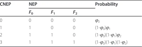
assume that there are three frames, each of which is coded to one packet, as depicted in Figure 1. In this fig-ure, the packet reference [1] is expressed by the arrows. Fk is the kth frame in temporal order, and Pk is its
coded packet. In this article, we define the number of effective packets (NEP) for each frame. The resulting distortions of the three frames are decided by the com-bination of NEP (CNEP) of the frames. For this coding structure, four CNEPs can be considered, as shown in Table 1. If a referenced packet is unavailable, any packet referencing it is also unavailable. For example, ifP0 is unavailable, P1 becomes unavailable, so that P2 also becomes unavailable. Therefore, if NEP forF0 is 0, all of the packets ofF1 andF2 become unavailable for decod-ing. Hence, NEPs forF1 andF2also become 0, as shown by the CNEP of 0. CNEP = 1 denotes the case whereP0 is available andP1 is unavailable. Therefore, the NEP for
F2 is also 0, becauseP2 becomes ineffective for distor-tion. The probability of occurrence of each CNEP is shown in the table in terms of the PLR of the packets. If
P0 is unavailable,P1andP2are also unavailable, so that CNEP = 0. In other words, the probability of CNEP = 0 is the same as the PLR ofP0, j0. As CNEP = 1 in the case where P0 is available and P1 is unavailable, the probability of CNEP = 1 is (1-j0)j1. In this way, the
probability of the four CNEPs can be calculated, so that the expected distortion of the three frames can be obtained from (1). Therefore, the expected distortion of
F0 is d¯0=φ0d0, 0+(1−φ0) φ1d0, 1+(1−φ0) (1−φ1) φ2d0, 2+(1−φ0) (1−φ1) (1−φ2)d0, 3.
As the distortion of F0 is not affected by the quality of F1 or F2, d0,1 = d0,2 = d0,3. There-fore,d¯0=φ0d0, 0+(1−φ0)d0, 1. In this way, the expected distortion of F1 can be written as
¯
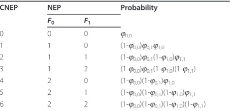
d1=φ0d1, 0+(1−φ0) φ1D1, 1+(1−φ0) (1−φ1)d1, 2, where d1,2 =d1,3. If we assume SVC, we can consider multiple layers [1]. Therefore, as shown in Figure 2, each frame can be coded to multiple packets, where each packet of a frame represents a spatial or quality layer. In this article, we focus on quality scalability and consider MGS coding. Therefore, in the rest of this arti-cle, the term“packet”means base quality layer packet or MGS packet. In Figure 2, Pk, l is thelth quality layer
packet ofFk, where the 0th quality layer means the base
layer. The associated CNEPs are given in Table 2. In the same way as the previous coding structure, the expected distortion ofF0can be obtained as
¯
d0=φ0, 0d0, 0+
1−φ0, 0
φ0, 1d0, 1+
1−φ0, 0 1−φ0, 1
d0, 4, (2)
whered0,1=d0,2 =d0,3and d0,4=d0,5=d0,6. In this way, the expected distortion of each frame can be expressed in terms of PLRs. The CNEPs in Table 2 can be categorized into three groups according to the num-ber of frames requiring error concealment, where a number of error concealment techniques [17] can be considered for any frame that NEP = 0. For example, CNEP = 0 requires concealment for both of the frames, whereas CNEP = 1 or 4 requires concealment for F1. Neither frame requires any error concealment for the remaining four CNEPs. Therefore, C (the number of CNEPs) for Figure 2 is 20 + 21 + 22 = 7. C can be gen-eralized as
C=Tt=0Qt, (3)
where T and Q are the number of frames and qual-ity layers, respectively. This analysis can be extended to more complicated coding structures, such as the hier-archical B structure [1].
P
0
F
0
P
1
F
1
P
2
F
2
Figure 1Reference structure of three frames.
Table 1 Possible CNEPs of the reference structure in Figure 1
CNEP NEP Probability
F0 F1 F2
0 0 0 0 j0
1 1 0 0 (1-j0)j1
2 1 1 0 (1-j0)(1-j1)j2
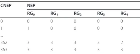
B. Expected distortion of hierarchical B structureFor further coding efficiency and temporal scalability, SVC is designed to provide the hierarchical B structure shown in Figure 3, where four temporal layers are pre-sented. To simplify the distortion analysis, this article defines reference groups (RGs), so that the hierarchical B structure in Figure 3 can be analyzed as depicted in Figure 4. In the figure, frames in an RG are independent of each other. Therefore, one RG can be considered as one frame in order to simplify the analysis of the refer-ence structure and calculate the video distortion (detailed discussion is given with Table 3). Although some of the references in Figure 3 are omitted in Figure 4, this representation can sufficiently describe the refer-ence relations. For example, we can see from Figure 4 thatF4cannot be decoded ifF0is not decoded, although the reference arrow fromF0 toF4is omitted in the fig-ure. The CNEP of a frame unit was introduced pre-viously. In this section, the CNEP of an RG unit is introduced in order to analyze the expected distortion of the hierarchical B coding structure. If the number of quality layers (including the base layer) is 3, the number of CNEPs is 364 according to (3), as T (the number of RGs in this case) is 5. Therefore, 364 decoding simula-tions, as listed in Table 3, must be accomplished to obtain d¯k for 0≤ k≤8, where the NEPs of frames in an
RG are the same as the NEP of the RG. For example, CNEP = 362 means that 2 packets are available for every frame in RG4 (F1, F3, F5, and F7) and 3 packets are available for the remaining frames. As each of the frames in an RG is independent of other frames in the same RG, these frames can independently be analyzed. For example, in order to calculate d¯1 (the expected dis-tortion of F1), the probability of each CNEP must be calculated. Therefore, the NEPs of RG0, RG1, RG2, RG3, and RG4 can be considered as the NEPs ofF0,F8,F4,F2,
and F1, respectively. The probability of each CNEP is then calculated based only on the PLRs of packets inF0,
F8, F4, F2, and F1, because d¯1 is not affected by the PLRs of packets in the other frames. The distortion of thekth frame of the cth CNEP,dk, c, can be calculated
from the simulation of thecth CNEP. For example, to calculate d1,362, one packet (the highest quality layer packet) for each frame in RG4 is eliminated, and all of the remaining packets are decoded. The resulting distor-tion ofF1can be obtained ford1,362. Note that the NEPs of framesF3, F5, and F7 in the same RG do not affect
d1,362. However, performing 364 decoding simulations to optimize 9 frames is impractical. Therefore, a more effi-cient version of this expected distortion analysis is required, as discussed in Section 3.5.
2.2.2. Increment of expected distortion
The increment in the expected distortion due to every packet loss must be obtained in order to minimize the expected distortion, as discussed in Section 3. As we have mentioned, the expected distortion can be expressed in terms of the PLR. Consequently, the increment can also be expressed in terms of the PLR. In Figure 2, for exam-ple, if the PLR ofP0,0increases, the expected distortion ofF0(d¯0 in (2)) increases according to
∂d¯0
∂φ0, 0
=d0, 0−φ0, 1d0, 1−
1−φ0, 1
d0, 4.
On the other hand, the PLR of P1,0, j1,0, is irrelevant to the expected distortion d¯0 given by (2), as no packet inF0referencesP1,0. Therefore,
∂d¯0
∂φ1, 0
= 0,
as (2) does not containj1,0. In this way, the increment of the expected distortion can also be calculated for the hierarchical B structure, where the structure can be
P
0,1
F
0
P
0,0
P
1,1
F
1
P
1,0
Figure 2Reference structure of two frames with two quality layers.
Table 2 Possible CNEPs of the reference structure in Figure 2
CNEP NEP Probability
F0 F1
0 0 0 j0,0
1 1 0 (1-j0,0)j0,1j1,0
2 1 1 (1-j0,0)j0,1(1-j1,0)j1,1
3 1 2 (1-j0,0)j0,1(1-j1,0)(1-j1,1)
4 2 0 (1-j0,0)(1-j0,1)j1,0
5 2 1 (1-j0,0)(1-j0,1)(1-j1,0)j1,1
simplified by using the reference group concept dis-cussed in Section 2.2.1.
2.2.3. Expected delay
For Pi, the number of bits that can be transmitted per
second over thehth link isrlog2(μi, h), whererand μi, h
are the bandwidth and modulation level allocated toPi
over the hth link, respectively. Therefore, the expected time required to transmitPiover thehth link is
¯
τi,h= (
1−Yi)Li
rlog2μi,h
, (4)
whereLiand Yiare the number of bits and the PDR
of Pi, respectively. Note that τ¯i,h is the expected value,
asYiis a probability. Therefore, the delay constraint is
¯
τ =
Pi∈Pτ¯i,h≤T, (5)
where P={Pi|i= 0, 1. . .,N−1} is the set of packets in a GOP (N =F×Q is the number of packets in a GOP, where Q is the number of quality layers employed).
2.2.4. Optimization
The purpose of the proposed method is to minimize the average of the expected distortion of each frame in a GOP. Therefore,
¯
d= 1
F F−1
k=0
¯
dk,
where ℱis the number of frames in a GOP. The PLR of packetPiinPis
φi= 1−(1−Xi) (1−Yi), (6)
where Xiis the PER of Pi. Here, the Lagrange
optimi-zation formula can be written as
μ∗,Y∗,λ*= arg mind¯+λ (τ¯−T), (7)
where τ¯ and Tare the required and allowed delay in transmittingP, respectively.lis the Lagrange multiplier. As shown in (7), the optimized modulation level setμ*, PDR set Y*, and Lagrange multiplier l* must be found in order to minimize d¯+λ (τ¯−T).
3. Implementation of the proposed system
3.1. Resource distortion attribution
As discussed in [3], each additional MGS coded video packet drop results in an increment in the received video distortion and a decrement in the required bit rate. For each MGS packet, the study [3] defines
F
0
F
1
F
2
F
3
F
4
F
5
F
6
F
7
F
8
Figure 3Hierarchical B structure with four temporal layers.
RG
4
RG
3
RG
2
RG
1
RG
0
F
0
F
8
F
4
F
2
F
6
F
1
F
3
F
5
F
7
Figure 4Reference group representation of Figure 3.
Table 3 CNEPs of the RG structure in Figure 4
CNEP NEP
RG0 RG1 RG2 RG3 RG4
0 0 0 0 0 0
1 1 0 0 0 0
...
362 3 3 3 3 2
For bit rate control, the packets are prioritized accord-ing to the RD attribute. In this article, we modify this to consider the required time resource (delay). Any incre-ment in the PDR or modulation level results in an increment in the expected distortion and a decrement in the required delay. Therefore, this article defines the resource-distortion (RsD) attribute, which is the distor-tion increment/delay decrement, as
λPHY
xi, hcan be approximated as
xi,h ≈0.2 exp
for multi-level quadrature amplitude modulation (MQAM), wheresi, his the SNR of the hop. In (9),Xiis
the PER at the destination node, which is
Xi= 1−
where ℋ is the number of hops in the path. There-fore, Equation (9) is
∂d¯
Note that if Yiis 1, both the dividend and divisor of
λPHY
i,h are 0, so that λ
PHY
i,h cannot be specified. In other
words, λPHYi,h can take any value. On the other hand, the
From (4), the divisor is
−∂∂τ¯
Note thatYiis a probability, and can be controlled to
take an edge value of 0 or 1 by the transmitter. If it is one of these two edge values, neither the dividend nor the divisor of λMACi can be specified. Consequently,
λMAC
i cannot be specified, which means it can take any
value.
3.2. Algorithm I–searching continuous modulation level and PDR
Ifμ* and Y* minimize d¯+λ (τ¯−T) in the optimization formula (7) differentiated with respect to any elementμi,
hinμ* andYiinY* becomes 0, so that
The equations above can be reformed and substituted with RsD attributes as
λ=λPHY
i,h =λ
MAC
i . (15)
As Yi affects λPHYi,h and λMACi , as shown in (13) and
(14), the following three settings can be considered in order to satisfy (15).
•Setting 1: Setμi, hto satisfy (15) andYito 0 <Yi< 1.
•Setting 2: Setμi, hto satisfy λ=λPHYi,h andYito 0.
The target service of the proposed method is real-time streaming that requires a more stringent delay con-straint than that on the expected delay given in (5). However, Yi is not 0 or 1 for Setting 1, which means
thatPimay or may not be sent. Therefore, by excluding
Setting 1 from our consideration, Equation (5) can be modified to
τ =
Pi∈P
(1−Yi) τi,h≤T, whereYi∈ {0, 1}. (16)
Therefore, Algorithm I considers only Settings 2 and 3. Algorithm I is developed to searchμi, hso as to make
λPHY
i,h approachesl. From (10),μi, hcan be evaluated in
terms ofxi, has 1-1.6si, h/ln[xi, h]. Therefore, μi, h
satis-fying (15) can be determined by obtainingxi, hsatisfying
(15). xi, h is the BER value, which is usually close to 0.
Thus, it is convenient to consider the logarithmic values
bi, h= ln(xi, h) and i,h = ln
is the term independent of bi, h and its logarithm,
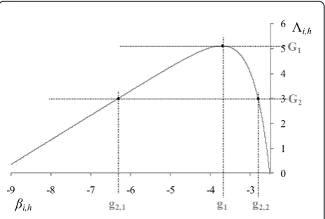
respectively. Figure 5 provides an example of Λi, h,
where Li and Ψi, h are set to 5000 and 6, respectively.
To calculate xi, haccording to (10),si, his set to 15 dB.
If inputΛ(the value that Λi, hshould approach) is G1, the solution of bi, h is g1. However, if input Λis G2,
there are two candidate solutions forbi, h, which are g2,1
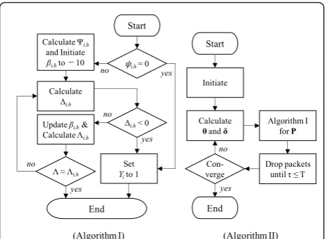
and g2,2. In this case, the lower value g2,1is selected, as the purpose of the algorithm is to minimize δ¯. To find the intersection, Algorithm I is developed as shown in Figure 6. The second term in (17) is ln(μi, h) + (Li-1) ln
by differentiating each term in (17) with respect tobi,
h. Note that Ψi, h has vanished, as it is independent of bi, h. First, Algorithm I checks whether or notψi, his 0,
whereas Algorithm II calculatesθi, hand δ¯i according to
(11) and as discussed in Section 2.2.2, respectively, then inputs those values to Algorithm I. If at least one of the packets referenced by Pi is dropped, δ¯i becomes 0
because a change inji cannot contribute to d¯.
Conse-quently, ψi, hbecomes 0 and Λi, h becomes -∞,
regard-less ofbi, h, according to (18). This means that a value
of bi, h satisfying (15) does not exist. Therefore,
Algo-rithm I setsYi to 1, i.e., Setting 3, in order to drop the
packet and satisfy (15) regardless of bi, h. Otherwise, if ¯
d is not 0, Ψi, his calculated from ψi, h according to
(18) in order to obtain the intersection shown in Figure 5. It can be seen from Figure 5 that the intersection of the curveΛi, h and the solution, e.g., g1 or g2,1 (rather
than g2,2), must be somewhere at whichΔi, h≥ 0 (note
that the slope at the intersection of Δi, h and g2,2 is
negative, and that the solution g2,2 maximizes the video distortion, which is not desired). Therefore, bi, hshould
initially be set to a sufficiently small value. We found that bi, h = -10 (xi, h = 10-10) was sufficiently small to
make the slope positive for various settings of Li, Ψi, h,
andsi, h. To reduce the computational power, the
algo-rithm utilizes Δi, h. IfΔi, his negative,Yiis set to 1 and
the process is terminated. Otherwise,bi, his increased
by (Λ-Λi, h)/Δi, hto allowΛi, hto approach Λ. IfΛi, his
within a predefined tolerance of Λ, we consider bi, h
satisfying (15) to have been found. Otherwise, we repeat the iterations of calculating Δi, h andbi, huntil Λi, h
becomes close to Λ. A small number of such iterations are sufficient to approach the solution, becauseΔi, h has
an almost constant value of 1 for lowbi, h, e.g., lower
than approximately -4.5 in Figure 5. This is due to the second and third terms in (19) becoming very small compared to 1 as xi, happroaches 0. However, if the
inputΛis higher than the possible maximum ofΛi, h, e.
g., Λ> G1 in Figure 5, the solution does not exist. In this case,Δi, hbecomes negative while the Δi, h andbi, h
calculations are repeated. Table 4 shows an example where the inputΛis set to 6 for Figure 5.
As shown in Table 4,bi, h was initially set to -10, as
depicted in Algorithm I in Figure 6. In the first iteration of Algorithm I, Δi, h and Λi, h are calculated to be
0.9935 and -0.6443 according to (17) and (19), respec-tively. Λi, h = -0.6443 is not close to Λ = 6, so
Algo-rithm I determinesΔi, h, and finds that it is negative.
Therefore, Algorithm I is terminated by setting the PDR
Yito 1, which means thatPiwill be dropped.
3.3. Algorithm II–refining parameters
In Algorithm I, δ¯i, andθi, hare used to calculate ψi, h
according to (18). δ¯i is affected by the PLR of packets referenced byPi and the PLRs of packets referencingPi.
In addition,θi, h is affected by the PERs ofPiof other
links, according to (11). However, δ and θ (which are the set of δ¯i andθi, h forP, respectively) are not
avail-able unless Algorithm I has been accomplished for the related packets and links so far. Therefore, this article proposes Algorithm II, which initializes the PDR and PER of every packet over every link to 0 in order to initiate δandθ. Therefore, Algorithm I can calculateμ and Y over the packets. However, if μ and Y do not
satisfy (16), a real-time streaming service cannot be guaranteed. Therefore, Algorithm II drops packets with Setting 2 until (16) is satisfied, as shown in Figure 6. Equation (14) can be used as the criterion for deciding which packets will be dropped, as it quantifies the attri-bute of transmittingPi. Therefore, it drops packets with
a lower λMACi . In this way, the setY obtained by Algo-rithm I overPis modified according to the packet drop-ping procedure. Using the obtained PDR setY and the PERs that can be calculated by μ, the algorithm can renew δ and θ. μ and Y are then calculated again via the same procedure. If every element pair in the pre-viously calculated μ and Y is close to corresponding with those in the new μ andY, we consider (15) to be satisfied. Therefore, Algorithm II is terminated. Other-wise, the algorithm repeats this procedure untilμ andY become stable.
3.4. Algorithm III–satisfying the resource constraint
Figure 7 shows some examples of output from Algo-rithm II in terms of (a) the number of packets trans-mitted, (b) the required delay for transmitting the packets, and (c) the expected peak SNR (EPSNR), where
EPSNR = 10log10 255
2
¯
d
.
The expected distortion d¯ is calculated in terms of mean squared error (MSE). The allowed delayTin (16) is set to 0.2 s. Using the example of Figure 7, this sec-tion discusses Algorithm III, which is designed to find the value of Λ that maximizes EPSNR, where the EPSNR performance of Algorithm II for various inputΛ is shown in Figure 7c. The reason for the local maxima of EPSNR in Figure 7c is as follows. If Λ= 2.6, Algo-rithm II allocates 19 packets to transmit and a 0.194-s transmission time (by modulation setting for the 19 packets), as shown in Figure 7a, b. As the allowed delay is set to 0.2 s, more transmission time can be allocated by adjusting Λ. By reducing Λ from 2.6, the BER for
ɗi,h= 0
(Algorithm I) (Algorithm II)
Figure 6Algorithms for findingμand Y for a givenΛ.
Table 4 Calculations forΛi, hto approachΛ= 6 in Figure 5
Iteration bi, h Λi, h Δi, h
1 -10 -0.6443 0.9935
2 -1.4876
each transmitted packet is lowered (as shown in Figure 5), which means that a lower modulation level is allo-cated. Therefore, the transmission time becomes larger by reducingΛ from 2.6, as shown in Figure 7b. AsΛ approaches 2.4, the transmission time approaches its maximum of 0.2 s. However, if Λis less than 2.4, the number of transmitted packets is reduced to 18, as shown in Figure 7a, to keep the transmission time below 0.2 s. Thus, the transmission time is reduced dis-continuously, as shown in Figure 7b. These discontinu-ities in radio resource (transmission time) result in the discontinuities and local EPSNR maxima observed in Figure 7c. Algorithm III is designed to find theΛvalue that maximizes EPSNR. In the rest of this section, Algo-rithm III is explained by reference to the EPSNR perfor-mance of Figure 7c. In order to avoid the local maxima in the figure, Algorithm III iteratively reduces the search range. In the first iteration (Iteration 1 in Figure 7c), three equally spaced initialΛvalues are selected. In the figure, these three values are 2, 2.65, and 3.3, where the values are chosen for the purpose of visual convenience. (If the EPSNR maximum does not exist between 2 and 3.3, the maximum cannot be found with these initial values. Therefore, a sufficiently wide range for the initial values of -10, 0, and 10 is considered in the simulations of Section 4.) Of the three EPSNRs with these initial values, that with Λ= 2.65 is the greatest. Therefore, in the next iteration (Iteration 2), two more Λ values (2.325 and 2.975, which make the interval 0.65/2 = 0.325 for the five Λ values of Iterations 1 and 2) are chosen around 2.65, and EPSNRs for the two new Λ values are determined by Algorithm II. In Iteration 3, two more Λ values (2.8125 and 3.1375) are chosen around Λ = 2.975, which gave the greatest EPSNR among the five Λ values of Iterations 1 and 2, and EPSNRs for these two values are determined. In this way, two moreΛvalues are tested in the next iteration, and the same procedure is repeated until the predefined number of iterations is accomplished. TheΛvalue with the greatest EPSNR among all tested values is then cho-sen for the packet transmission.
3.5. Practical expected distortion and increment
The expected distortion and its increment are discussed in Section 2. The expected distortion increment δ¯i is utilized to find the optimal packet extraction and modu-lation level allocation, and is updated while Algorithm II is performed. To obtain the exact amount of the expected distortion, the number of error patterns given by (3) must be simulated, which is impractical as T and Q grow. Therefore, the number of simulations must be reduced for practical implementation. For example, we can simulate only the T Q+ 1 CNEP that are most
likely to occur at the destination node. Table 5 shows an example of the CNEPs where the number of tem-poral layers and quality layers are 2 and 2, respectively. If the NEPs in the temporal level immediately before the current level is the same as or 1 greater than that of the current level, the CNEP is chosen in order to calcu-lateδ (for Algorithm II) and d¯ (for Algorithm III). In this case, T = 3, so that the number of required CNEPs is 7 =T Q+ 1, as in Table 5. In the case of T = 5 and Q= 3, it is 16, which is much more practical than the 364 simulations discussed in Section 2.2.1.
3.6. Complexity of the proposed method
The proposed method consists of three algorithm levels. As shown in Figure 6, Algorithm II runs Algorithm I as many as HP times until the convergence criterion for Algorithm II is achieved. Therefore, the complexity of Algorithm II is κ2=HP(κ1+κMAC) η2, where 1 and
MACare the complexity of Algorithm I and the calcula-tion of (14) for the packet dropping module in Algo-rithm II, respectively. h2 is the number of iterations required for convergence. The complexity of Algorithm I is1=0h1, where0is the complexity of calculating (17) and (19) and h1 is the number of calculations. As Ψiis fixed for each iteration of Algorithm I, the
calcula-tion of the second term in (17) is the main cause of the complexity. The computational power required to calcu-late this term is mainly dependent on calculating 10βi,h
to obtain xi, h, ln(5xi, h), ln(μi, h), and
x∗i,h
Li−1 . Once
its components have been calculated, Equation (19) can easily be obtained. AsMAC is trivial compared to1,2 can be considered as HPκ1η2. Consequently, the total complexity for the proposed method for optimizingPis κ =HPκ0η1η2η3, whereh3is the predefined number of samples taken to find the optimal Λ, as discussed in Section 3.4. Therefore,can be considered as O(HP).
3.7. Algorithm I–discrete-searching discrete modulation level and PDR
Section 3.2 introduced Algorithm I for finding a contin-uous modulation level and PDR for a packet. Algorithm I finds a continuous modulation level satisfying
λ=λPHY
i,h . However, it is not practical to realize this
tinuous modulation value. Therefore, this section con-siders discrete modulation levels affordable by MQAM. For instance, five modulations, such as 4-, 16-, 64-, 256-, and 1024-QAM256-, can be considered. By reforming (10)256-,
bi, hcan be written as
βi,h=C1+ C
2σi
1−μi,h
Constants C1 and C2 are log10[0.2] and 1.6/ln[10], respectively. As M= {4,16,64,256,1024}, the number of possiblebi, h, and consequently the number of possible
Λi, h, is also five. Hence, it is difficult to satisfy
λ=λPHY
i,h . Therefore, an alternative method (Algorithm
I–Discrete) is considered, which finds the Λi, hclosest
toΛ from among the five possible candidates. Conse-quently, modulation levels with Δi, h ≥ 0 are selected
from the five candidates, and the level whoseΛi, h value
is closest toΛis found. However, if each of the five can-didates is less than 0, it can be considered that none of the modulation levels is adequate. Therefore, the algo-rithm sets the PDR to 0 and terminates. By substituting Algorithm I (which is called by Algorithm II, as in Fig-ure 6) with Algorithm I–Discrete, an efficient packet extraction and discrete modulation level scheme can be obtained by Algorithm III.
4. Simulation results
4.1. Transmission path configured with a single link
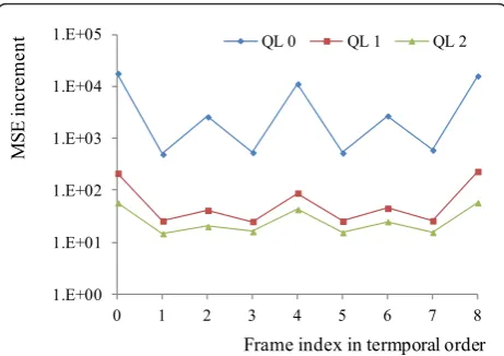
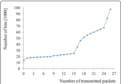
Prior to a discussion of multi-link cases, the perfor-mance of the proposed method for a single link is dis-cussed. The proposed method is designed to find the optimal set of transmitted packets, and the modulation level of each transmitted packet, for a transmission path configured with multiple links. Therefore, if the pro-posed method is applied to a single link, it operates similarly to the method in [12], which is designed to determine the optimal set of transmitted packets and transmission modes. In the rest of this article, the two methods are termed Single Link Optimization (SLO) and Multi-Link Optimization (MLO). In this section, JSVM 9.19.7 [17] is considered for the simulations. For the simulations of Sections 4.1 and 4.2, Mobile common intermediate format (CIF) is tested at 30 frames per sec-ond (FPS) with a bandwidth of 150 kHz for each link, where the GOP size is 8 (which results in three tem-poral layers (TLs) in the hierarchical B structure, as in Figure 3) and the number of quality layers (QLs) is 3. Figure 8 shows the total MSE increment of the first
GOP by excluding each of the 27 packets configuring 9 frames and 3 QLs (QL 0, QL 1, and QL 2), where QL 0 is the base quality layer and the ninth frame is shared by the next GOP. If we consider an adaptive modulation strategy to guarantee a fixed BER level for every link, the number of transmitted packets for the limited trans-mission time (0.2 s in this section) is determined by the BER level. If the BER level is lowered to reduce channel error, the bit rate is reduced, so that the number of packets transmitted is reduced. Figure 9 shows the num-ber of bits according to the numnum-ber of transmitted pack-ets, where the 27 packets of Figure 9 are prioritized by RD attribution, as in [3]. Figure 10 shows the number of the transmitted packets with respect to the channel SNR, where the target BER is set to either 10-7, 10-8, or 10-9. As shown in Figure 10, more packets can be trans-mitted by considering a higher BER level. The transmis-sion time for the three BER levels of the adaptive modulation strategies are shown in Figure 11a. If a BER level is set for the packets, the transmission time is determined solely by the number of packets. Therefore, the allowed time of 0.2 s is not fully utilized in most cases, as shown in Figure 11a. Consequently, it is unfair to compare the three BER levels of the adaptive modula-tions with the proposed method, as the proposed method is designed to fully utilize the given transmis-sion time. Therefore, this paper considers a Flexible BER Decision FBeD method, which finds the BER level that minimizes the expected video distortion when applied to all transmitted packets. FBeD is considered to provide a performance upper bound to the adaptive modulation method designed to guarantee a fixed BER level, and FBeD shows better performance than the other three methods in terms of EPSNR, as shown in Figure 11b. Furthermore, as FBeD can fully utilize the Table 5 Reduced number of CNEPs considered for
practical implementation
CNEP NEP
F0 F1 TL1
0 0 0 0
1 1 0 0
2 1 1 0
3 1 1 1
4 2 1 1
5 2 2 1
6 2 2 2
1.E+00 1.E+01 1.E+02 1.E+03 1.E+04 1.E+05
0 1 2 3 4 5 6 7 8
QL 0 QL 1 QL 2
M
SE
in
cr
emen
t
Frame index in termporal order
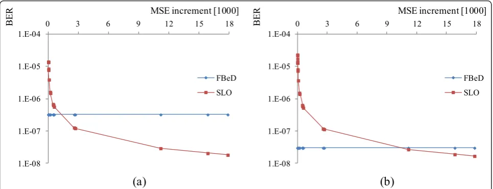
given transmission time, as shown in Figure 11a, it is suitable for comparison with the proposed method. Meanwhile, the proposed method individually deter-mines the BER level for each packet according to its dis-tortion increment (MSE increment) and bit length. Figure 12 shows the allocated BER of each packet and its MSE increment for FBeD and SLO with channel SNRs of 12 and 14 dB. The cumulative transmission time for each transmitted packet using the two methods is shown in Figure 13, where the cumulative time is considered to show the total transmission time reaching 0.2 s. In Figure 13, the transmitted packets are sorted in decreasing order of MSE increment, so that it can be conveniently observed alongside Figure 12. For a 12-dB channel SNR, both FBeD and SLO transmit 17 packets. In the 14 dB case, FBeD and SLO transmit 19 and 22 packets, respectively. As shown in Figure 12a, SLO pro-vides higher protection for 4 of the 17 packets, and more time is allocated for the packets with a high MSE increment, as shown in Figure 13a, where the number of transmitted packets is the same. As shown in Figure 12b, SLO allocates a higher BER for 19 of the 22 pack-ets, so that it allocates less time for packets with a low MSE increment, as shown in Figure 13b. Hence, SLO can transmit three packets more than FBeD while pro-viding a lower BER level for three packets with a high MSE increment. For both values of the channel SNR, SLO shows better performance. This is shown in Figure 14, which shows the number of transmitted packets and EPSNR for various channel SNR cases.
4.2. Transmission path configured with two links
Whereas SLO finds the optimal transmission packet set and BER (modulation level) for a single link, MLO finds these two parameters for multi-links. In the following
0
Number of transmitted packets
N
Figure 9 Number of bits according to the number of transmitted packets for the 27 packets of Figure 8.
Figure 10Number of packets transmitted in 0.2 s with respect to channel SNR for various target BER.
0.13
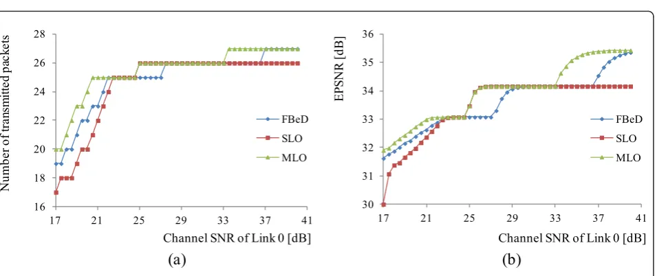
simulations, a transmission path configured with multiple links is considered, where the channel SNR of one link on the path changes. In Section 4.2, a transmission path configured with two links (Links 0 and 1) is considered in which the channel SNR of Link 1 is 25 dB and that of Link 0 varies. Figure 15 shows the transmission time used for each link to transmit all of the packets. In Figure 15, it can be seen that less time is allocated to a link with a relatively high SNR, so that the other link can use more time to protect the packets from channel error. For SLO, however, an equal time of 0.1 s is assumed to be allo-cated to each link, as it is designed for a single link. For multi-links, FBeD is adjusted to allocate the same BER level to all links, so that the transmission time can be flexibly allocated to each link, as in MLO. Figure 16
shows the number of transmitted packets and EPSNR with respect to a varying channel SNR of Link 0. As the same amount of time is allocated to each link when the SNRs of the links are the same, as shown in Figure 15, MLO shows a similar performance to SLO, as shown in Figure 16b. As shown in Figure 16, if the SNR difference between the two links is relatively small (i.e., SNR of Link 0 is 23-33 dB), the EPSNR performance of SLO and MLO is almost identical. In this case, the EPSNRs are higher than that of FBeD. However, as a link with a lower SNR cannot occupy more time in SLO, the EPSNR cannot be improved, even for Link 0 with a channel SNR above 33 dB. When Link 0 has a SNR below 23 dB, Link 0 cannot occupy more time in SLO, so that its EPSNR degrades to below that of FBeD.
(a)
(b)
1.E-08 1.E-07 1.E-06 1.E-05 1.E-04
0 3 6 9 12 15 18
FBeD SLO
MSE increment [1000]
BE
R
1.E-08 1.E-07 1.E-06 1.E-05 1.E-04
0 3 6 9 12 15 18
FBeD SLO
MSE increment [1000]
BE
R
Figure 12MSE increment and BER levels allocated by FBeD and SLO for transmitted packets among the 27 in Figure 8, where the channel SNR is (a) 12 dB and (b) 14 dB.
(a)
(b)
0.04 0.06 0.08 0.1 0.12 0.14 0.16 0.18 0.2
0 3 6 9 12 15 18 21 24 27
FBeD SLO
Transmitted packets, in decreasing order of MSE increment
Cu
m
ul
at
ive
tr
an
sm
iss
ion t
ime
[s
ec
ond
]
0.04 0.06 0.08 0.1 0.12 0.14 0.16 0.18 0.2
0 3 6 9 12 15 18 21 24 27
FBeD SLO
C
um
ula
tiv
e tr
an
sm
is
sio
n
tim
e
[s
ec
ond
]
Transmitted packets, in decreasing order of MSE increment
4.3. Transmission path configured with three links
In Figure 17, a path with three links (Links 0, 1, and 2) is considered, where the channel SNRs of Links 1 and 2 are 25 and 30 dB, respectively. Because the EPSNR per-formance of SLO is sensitive to an imbalance in the channel SNRs of links, SLO becomes more inadequate as the number of links grows. Therefore, the perfor-mance of SLO has been omitted from Figure 17. This figure shows the test results from three quarter CIF (QCIF)-15 FPS and three CIF-30 FPS videos, where the bandwidth for each link was set to 50 kbps for QCIF videos and 200 kbps for CIF videos. The GOP size for QCIF videos was set to 4 and that for CIF videos was set to 8. In addition to the two methods with continu-ous modulation levels (FBeD (CNT), MLO (CNT)), the performance of the methods with discrete modulation levels (as discussed in Section 3.7) is also shown in
(b)
Figure 14Performances of FBeD and SLO in terms of (a) Number of transmitted packets and (b) EPSNR.
Link 1 (Channel SNR=25dB)
Channel SNR of Link 0 [dB]
Tr
Figure 15Transmission time for each link, where the channel SNR of Link 1 is 25 dB.
Channel SNR of Link 0 [dB]
N
Channel SNR of Link 0 [dB]
E
Figure 17. For the six graphs in Figure 17, MLO (CNT) shows better performance than FBeD (CNT). In both the QCIF and CIF cases, Foreman shows acceptable video quality (EPSNR higher than 30 dB) for relatively low channel SNR compared to Mobile and Football for FBeD (CNT) and MLO (CNT). This is because the
visual and motion characteristics of Foreman are rela-tively simple compared to Mobile and Football, so it can be compressed more. Therefore, a lower modulation level can be allocated for Foreman while transmitting as many packets as required for acceptable video quality. However, as shown in Figure 17c, f, continuous
(a)
(d)
Channel SNR of Link 0 [dB]
E
Channel SNR of Link 0 [dB]
E
Channel SNR of Link 0 [dB]
E
Channel SNR of Link 0 [dB]
E
Channel SNR of Link 0 [dB]
E
Channel SNR of Link 0 [dB]
E
modulation levels below that supported by discrete MQAM (μi, hless than 4 in (20)) are evaluated by FBeD
and MLO for low channel SNR, so that FBeD (DSC) and MLO (DSC) degrade severely as the channel SNR degrades. Nevertheless, it is observed that MLO (DSC) shows improvement over MLO (DSC) for the six video sequences.
5. Conclusions
This article proposed a method to jointly exploit the bit rate and channel adaptation provided by MGS and adaptive modulation over a transmission path consisting of multiple wireless links. The proposed algorithms found the optimal packet transmission scheme by extracting packets according to an RsD attribution quantified as the distortion increment over the delay decrement. In order for the extracted packets to be transmitted, the proposed algorithms also found the optimal modulation allocation. The two factors of packet extraction and modulation allocation were opti-mized simultaneously by solving an optimization pro-blem to minimize the total distortion.
Abbreviations
BER: bit error rate; CDMA: code division multiple access; CIF: common intermediate format; CLO: cross-layer optimization; CNEP: combinations of number of effective packets; CSI: channel state information; EPSNR: expected peak signal-to-noise ratio; FPS: frames per second; GOP: group of pictures; MGS: medium grain scalability; MLO: link optimization; MQAM: multi-level quadrature amplitude modulation; MSE: mean squared error; NAL: network abstraction layer; NEP: number of effective packets; PDR: packet drop rate; PER: packet error rate; PHY: physical layer; PLR: packet loss rate; RD: rate distortion; RG: reference group; RsD: resource distortion; SLO: single link optimization; SNR: signal-to-noise ratio; SVC: scalable video coding; UEP: unequal protection.
Author details
1Advanced Wireless Communication Research Center, University of
Electro-Communications, Tokyo, Japan2Department of Radio-Communications,
Kyunghee University, Seoul, Korea
Competing interests
The authors declare that they have no competing interests.
Received: 15 July 2011 Accepted: 14 March 2012 Published: 14 March 2012
References
1. H Schwarz, D Marpe, T Wiegand, Overview of the scalable video coding extension of the H.264/AVC standard. IEEE Trans Circ Syst Video Technol.
17(9), 1103–1120 (2007)
2. T Schierl, T Stockhammer, T Wiegand, Mobile video transmission using scalable video coding. IEEE Trans Circ Syst Video Technol.17(9), 1204–1217 (2007)
3. I Amonou, N Cammas, S Kervadec, S Pateux, Optimized rate-distortion extraction with quality layers in the scalable extension of H.264/AVC. IEEE Trans Circ Syst Video Technol.17(9), 1186–1193 (2007)
4. CH Foh, Y Zhang, Z Ni, J Cai, KN Ngan, Optimized cross-layer design for scalable video transmission over the IEEE 802.11e networks. IEEE Trans Circ Syst Video Technol.17(12), 1665–1678 (2007)
5. G Cheung, A Zakhor, Bit allocation for joint source/channel coding of scalable video. IEEE Trans Image Process.9(3), 340–356 (2000). doi:10.1109/ 83.826773
6. E Maani, AK Katsaggelos, Unequal error protection for robust streaming of scalable video over packet lossy networks. IEEE Trans Circ Syst Video Technol.20(3), 407–416 (2010)
7. N Nejati, H Yousefizadeh, H Jafarkhani, Distortion optimal transmission of multi-layered FGS video over wireless channels. IEEE Trans Sel Areas Commun.28(3), 510–519 (2010)
8. LP Kondi, D Srinivasan, DA Pados, SN Batalama, Layered video transmission over wireless multirate DS-CDMA links. IEEE Trans Circ Syst Video Technol.
15(12), 1629–1637 (2005)
9. G Su, Z Han, M Wu, A scalable multiuser framework for video over OFDM networks: fairness and efficiency. IEEE Trans Circ Syst Video Technol.16(10), 1217–1231 (2006)
10. H Ha, C Yim, Y Kim, Cross-layer multiuser resource allocation for video communication over OFDM networks. EURASIP J Comput Commun.31(15), 3553–3563 (2008). doi:10.1016/j.comcom.2008.05.010
11. YP Fallah, H Mansour, S Khan, P Nasiopoulos, HM Alnuweiri, A link adaptation scheme for efficient transmission of H.264 scalable video over multirate WLANs. IEEE Trans Circ Syst Video Technol.18(7), 875–887 (2008) 12. H Mansour, YP Fallah, P Nasiopoulos, V Krishnamurthy, Dynamic resource
allocation for MGS H.264/AVC video transmission over link-adaptive networks. IEEE Trans Multimedia.11(8), 1478–1491 (2009)
13. N Mastronarde, DS Turaga, M Schaar, Collaborative resource exchanges for peer-to-peer video streaming over wireless mesh networks. IEEE Trans Sel Areas Commun.25(1), 108–118 (2007)
14. T Xiaolin, Y Andreopoulos, M Schaar, Distortion-driven video streaming over multihop wireless networks with path diversity. IEEE Trans Mobile Comput.
6(12), 1343–1356 (2007)
15. Y Zhang, S Qin, Z He, Fine-granularity transmission distortion modeling for video packet scheduling over mesh networks. IEEE Trans Multimedia.12(1), 1–12 (2010)
16. Z Zhang, Z Hu, A Hai, D Lu, Performance study of error resilience with multiple reference frames in H.264/AVC in conditions of low bit-rate, in
ICEMI’09, pp. 3-298–3-301 (2009)
17. JSVM Software Manual, Version. JSVM 9.19.7 (January 2010)
18. ST Chung, AJ Goldsmith, Degrees of freedom in adaptive modulation: a unified view. IEEE Trans Commun.49(9), 1561–1571 (2002)
doi:10.1186/1687-1499-2012-105
Cite this article as:Kimet al.:Modulation level allocation for MGS streaming over a multihop wireless channel.EURASIP Journal on Wireless Communications and Networking20122012:105.
Submit your manuscript to a
journal and benefi t from:
7Convenient online submission 7Rigorous peer review
7Immediate publication on acceptance 7Open access: articles freely available online 7High visibility within the fi eld
7Retaining the copyright to your article