Volume 2009, Article ID 192985,17pages doi:10.1155/2009/192985
Research Article
Distributed Velocity-Dependent Protocol for
Multihop Cellular Sensor Networks
Deepthi Chander,
1Bhushan Jagyasi,
2U. B. Desai,
3and S. N. Merchant
11SPANN Lab, Electrical Engineering Department, Indian Institute of Technology Bombay, Powai, Mumbai 400076, India 2TCS Innovation Labs Mumbai, Tata Consultancy Services, Yantra Park, Thane 400601, India
3Indian Institute of Technology Hyderabad, Ordnance Factory Estate, Yeddumailaram, Andhra Pradesh 502205, India
Correspondence should be addressed to Deepthi Chander,[email protected]
Received 22 July 2009; Accepted 15 December 2009
Recommended by Wei Li
Cell phones are embedded with sensors form a Cellular Sensor Network which can be used to localize a moving event. The inherent mobility of the application and of the cell phone users warrants distributed structure-free data aggregation and on-the-fly routing. We propose a Distributed Velocity-Dependent (DVD) protocol to localize a moving event using a Multihop Cellular Sensor Network (MCSN). DVD is based on a novel form of connectivity determined by the waiting time of nodes for a Random Waypoint (RWP) distribution of cell phone users. This paper analyzes the time-stationary and spatial distribution of the proposed waiting time to explain the superior event localization and delay performances of DVD over the existing Randomized Waiting (RW) protocol. A sensitivity analysis is also performed to compare the performance of DVD with RW and the existing Centralized approach.
Copyright © 2009 Deepthi Chander et al. This is an open access article distributed under the Creative Commons Attribution License, which permits unrestricted use, distribution, and reproduction in any medium, provided the original work is properly cited.
1. Introduction
In recent years, the idea of people-centric sensing or
par-ticipatory sensing has gained considerable significance in urban environments. Ubiquitously used hand-held devices such as cell phones, when additionally empowered with
sensing capabilities, form Cellular Sensor Networks, [1–
5], which collaboratively serve an application. While the
cellular backbone resolves issues related to the deployment and provision of energy for the embedded sensors, the mobility of cell phone users provides improved coverage
and energy efficiency, [6,7]. Further, extensive research in
Multihop Cellular Networks (MCN)have demonstrated their improved coverage and network capacity over conventional
cellular networks, [8,9]. Therefore,Multihop Cellular Sensor
Networks (MCSN), where sensor networks are built upon the MCN infrastructure, are advocated in this paper. The
schematic of a MCSN is shown inFigure 1. Here, cell phones
embedded with sensors transmit sensed data to the BS in a multihopmanner. A typical MCSN can cater to applications like environmental monitoring, urban planning, natural
resource management, civic hazard detection and infor-mation sharing. Some of the ongoing projects on various applications of Cellular Sensor Networks are summarized in Section 7.
In our work, we consider a moving event localization
application of Multihop Cellular Sensor Networks. The moving event that needs to be detected and localized can be gaseous leakage, toxic clouds, or a phenomenon like cyclone or dust storm. In all these applications, since the event as well as sensor nodes are mobile, a new set of nodes detect the event at every instant. Moreover, due to the extensive use of cell phones, enormous data will be generated in the network. For such scenarios, a centralized data aggregation scheme may not be suitable, due to the resulting energy loss and network congestion. Hence, the development of
an efficient distributed data aggregation scheme becomes
essential. Further, the mobility of the event as well as that
of the users entails the design of anon-the-fly protocol for
routing.
The problem of tracking mobile events using Cellular
Control messages
Relay node Aggregator Data
End-user Region of interest
Base station
Figure1: Schematic of a Multihop Cellular Sensor Network.
distributed tracking system called MetroTrack (details of
which are currently unavailable). In [4], the issues of
time-varying coverage of the event and time-varying mobile phone den-sity are tackled by a distributed Kalman-Consensus filtering algorithm. We however deal with these issues by proposing a Multihop Cellular Sensor Network based framework for
localizing the moving event. In [10,11], a moving
point-source target was tracked by static sensor nodes using a
cluster membership update mechanism and a tree-based approach, respectively. However in a MCN backbone, such a structured approach would incur large communication and computation overhead in structure formation and
maintenance. This motivates the idea of a structure-free
approach for aggregation and routing in MCSN. In [12], a
structure-free Data AwareRandomized Waiting (RW) time
protocol had been proposed for detecting a moving target using a static wireless sensor network.
The main contributions of our paper are as follows. (i) Use of a Multihop Cellular Sensor Network (MCSN)
for moving event localization.
(ii) Development of a novel Distributed
Velocity-Dependent (DVD) Waiting Time protocol for MCSN.
(iii) Analysis of the DVD protocol in terms of the time-stationary probability density function and the spatial distribution of waiting time.
(iv) Perturbation analysis of DVD considering perturba-tions in location, velocity and sensed data informa-tion at nodes.
The salient features of the proposed DVD protocol are as follows.
(i)Structure-Free. A distributed structure-free data aggregation is performed in DVD.
(ii)Moving Event and Mobile Nodes. In [12], nodes were located at fixed inter-node distances and a moving event was considered. In DVD, we localize
the trajectory of a moving event using data gathered by cell phone users.
(iii)Velocity-Dependent Waiting Time: Due to lack of
structure, the time for which a node delays transmis-sion of its own data in order to promote aggregation, cannot be ascertained a priori without some topology information. In the location-aware, structure-free
protocol proposed in [12], a Random Waiting Time
had been adopted. The Random Waypoint (RWP)
steady state distribution, [13], of users, is typically
observed in cellular networks. Therefore, in our work, we determine the waiting time based on the RWP mobility model. The proposed waiting time depends on location and velocity of nodes, resulting
in a better trade offbetween end-to-end delay and
connectivity (as explained inSection 3.2).
(iv)On-the-Fly Routing: Since we consider a dynamic scenario, the relaying of data is done independently
at each hop based on waiting time connectivity
(Section 3.1).
(v)Delay Minimization: To reduce end-to-end delay, routing of aggregated data at each hop is done by the node which has the minimum waiting time
amongst nodes that satisfywaiting time connectivity.
The spatial distribution of waiting time in DVD supports the relay node selection process, resulting in a low end-to-end delay.
The organization of the manuscript is as follows. In Section 2, the system model is described. A brief review of
the proposed DVD protocol [14], is described inSection 3. In
the current work, we derive the time-stationary probability density function and analyze the spatial distribution of waiting time to provide a better insight into the design and benefits of the proposed DVD protocol. These are discussed
in greater detail in Section 4 and Section 5, respectively.
To evaluate the robustness of DVD, we further perform a
sensitivity analysis to study the effect of perturbations on
sensed data, location or velocity measurements and obtain 95% confidence intervals for the average performances. Our
simulation results (Section 6) show that, with or without
perturbations, DVD performs better than RW in terms of
event localization error and end-to-end delay. The proposed DVD protocol and the existing Centralized scheme (Cellular Sensor Networks without multihop) have comparable event localization estimates. Even though the Centralized scheme has the lowest end-to-end delay, DVD is found to be
more energy-efficient than the centralized scheme.Section 8
concludes the paper.
2. System Model
2.1. Intensity Model. At any time instantt, the moving event
is defined by a location (center of event(CoE)) of maximum
event intensityIT, and the event radiusRe, within which the
event has an intensity greater than a threshold intensityID. In
general, moving events like gaseous leakage have an intensity
profile which decays with distance from the CoE, [15]. For
a nodeiat a distance ofde(i) from the CoE, the measured
intensityI(i) is given by
I(i)= IT(t)
4πde(i)2
, (1)
where the event intensityIT(t) at time instantt, is provided
by the application based on known models of the event, [15–
17]. An application-dependent event detection threshold
intensity ID, is also known at the user end. Node i is an
event node if it measures an intensity I(i) > ID and is a non-event node, otherwise. Every event node, computes its
distancede from the center of eventusing the known value
of event intensity IT(t) and its measured intensity I using
(1). It follows from (1) that all nodes within a distance of
Re(t)=
(IT(t))/(4π/ID) from thecenter of eventat timet,
areevent nodes.
2.2. Path Loss Model. We employ distance dependent variable
transmission power levels at nodes [18]. Ifr is the known
distance between source and destination nodes, using the
free-space path loss model of radiowave propagation, [19],
the transmission powerPt(r) at the source node is computed
as
where Pd is the minimum received power required for
successful reception at the destination. For a known receiver
sensitivitysin dBm, we computePd = 10s/10mW. λis the
wavelength of the Radio-frequency (RF) signal.
2.3. Energy Model of Mobile Phones. The sensing application is initiated by the mobile phone at regular sampling instants, as specified by the end-user. Between sampling instants, cell phone resources are used for regular (voice/text)
applica-tions. For any two time instants, t1 and t2, between two
Nodes acting
Figure2: Schematic of proposed DVD for moving event localiza-tion in Multihop Cellular Sensor Networks.
consecutive sampling instants, we assume that the residual
battery energyBdecays linearly in the following manner:
B(t2)=B(t1)−
(t2−t1)Bmax
Tmax .
(3)
In (3),Bmaxis the battery rating of the cell phone andt2> t1.
Tmaxis the corresponding talktime rating which determines
the maximum duration for which the cell phone can be powered while performing regular applications. Therefore,
assuming that a residual energy ofBmaxwould decay within
a time durationTmax, the energy drained within a duration
t2−t1would be ((t2−t1)Bmax)/Tmax.
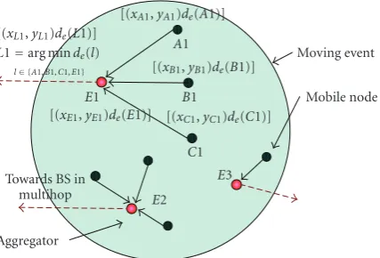
2.4. Aggregation Rule. Each aggregator selects the location
of the node with minimumde as its estimate of the center
of event, from among the event nodes that transmit data
to it. For anyevent node i, (xi,yi) is its location andde(i)
is its distance from CoE. From Figure 5, let S1 be the
set of event nodes (say A1,B1,C1) transmitting data to
an aggregator node E1, then by the aggregation rule, E1
estimates the location of thecenter of eventas (xL1,yL1) where
L1 = arg mini{de(i) : i ∈ S1}. AggregatorE1 transmits
[(xL1,yL1),de(L1)] to the BS. Note that the aggregation
rule is chosen to be computationally light on the resource-constrained cell phones. The BS makes the final estimate
of CoE by trilateration (for precise data) or aLeast Squares
approach (for imprecise data) using data obtained from
many such aggregators (E1,E2,E3 shown inFigure 5). Note
that the localization algorithm (trilateration/LS estimation) is implemented only at the BS which is assumed to have
sufficient power and computational capabilities.
3. Distributed Velocity-Dependent (DVD)
Waiting Time Based Protocol
In this section, we describe the proposed structure-free Distributed Velocity-Dependent (DVD) Waiting Time based
protocol used to aggregate sensed data and route it efficiently
0
Figure 3: Random Waypoint spatial distribution in Cellular Networks.
Figure 2shows the schematic of the proposed DVD protocol. The main challenges involved in the design of the protocol are:
(i)Dynamic Topology: This necessitates structure-free data aggregation and on-the-fly routing.
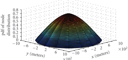
(ii)Non-uniform node distribution: Cell phone users, in general, closely follow a Random Waypoint
distribu-tion, [13], shown inFigure 3. The probability density
of the time-stationary distribution of mobile node
location,M(t) at a point (x,y), in a circular disk of
that the node density decreases from the center to the boundaries of the circular disk. Therefore, the protocol design must ensure connectivity of all nodes despite the non-uniformity in node distribution. To tackle this, we exploit variable waiting times at nodes, which will be discussed in the following subsections.
3.1. Waiting Time Connectivity in DVD. Each node is
associated with a waiting timeτ. Duringτ, the node waits
to receive data from other nodes for aggregation or relaying, and transmits the data at the end of its waiting time. Connectivity in DVD is defined based on the waiting time of
nodes. We propose the followingWaiting Time Connectivity
(WTC) rule:
Letτ(i) be the waiting time of node i and di j be the
Euclidean distance between nodeiand nodej. For nodejto
successfully transmit to nodei, the following condition must
hold:
τ(i)>2di j
c , (5)
wherecis the radiowave propagation velocity. Alternately,i
is connected to jif waiting time ofi,τ(i), is greater than the
round-trip propagation delay from j toi. Foriconnected to
j, (5) implies the following.
Implication (a). Ifτ(i) is large,di j can be largeyet ensuring
that nodejsuccessfully transmits toi. In this case nodeican
receive data even from distant nodes and is said to have high connectivity.
Implication (b). Ifτ(i) is small,di j must be smallto ensure
successful transmission from node j to i. Thus node i
can receive data only from nearby nodes and has low connectivity. Note that the WTC rule is in general non-reciprocal.
3.2. Waiting Time in DVD. Connectivity is essential in order to favor aggregations and to successfully relay aggregated data to the BS requiring nodes to have large waiting times. At the same time, very large waiting times lead to an increase in end-to-end delay, as the data gets released slowly by each intermediate node in the network. Thus, the design of
waiting time is a trade-off between end-to-end delay and
connectivity. In DVD, data aggregation is done byevent nodes
while relaying of aggregated data is done bynon-event nodes
(Figure 2). A node chooses its waiting time depending on
whether it is anevent nodeor anon-event node.
During its waiting time, anevent nodeacting as
aggre-gator waits to receive data from other event nodes for
aggregation, and transmits its data to a relay node thereafter.
For anevent node,i, the waiting timeτ(i)= τe(i), which is
maximum velocity of nodes in the network andde(i) is the
estimated distance of nodeifrom the center of event. This
proposed definition ofτe(i) is explained as follows:
Distance from center of event. From (6), anevent nodeclose to thecenter of eventis given a low waiting time. This is because, the location information of such a node is critical and should be communicated to the BS at the earliest.
Instantaneous velocity . From (6), a slow-moving node has a
large waiting time. This permits it to beconnected todistant
nodes (Implication (a)) with a lesser chance of packet losses.
However, a fast moving node is permitted to receive data only from nearby nodes by assigning a low waiting time (Implication (b)) to it, thereby reducing packet losses.
During its waiting time, anon-event nodewaits to receive
aggregated data which is further relayed at the end of
its waiting time. For a non-event node, i, we propose the
following definition of waiting time,τn(i):
τn(i)=
times (Implication (a)) to ensure connectivity to them. Since node density is higher near the BS, nodes that relay data from sources near the BS can have small waiting times (Implication (b)). Therefore, waiting time ofnon-event nodes can progressively increase with distance from the sink. The
dependence ofτnon instantaneous velocity can be explained
as in the case ofτeforevent nodes.
3.3. Protocol Description. In this work, we estimate the trajectory of the moving event by localizing the center of event at regular sampling instants. Initially, an event is said to have occurred if a minimum number of nodes report event occurrence directly to the BS. If it decides in favor of event detection, on the basis of the reported intensities and locations of the cell phone users, the end-user application
estimates the temporal variation of event intensityIT(t), and
the sampling intervalTsusing known models of the event,
[15,16]. The sensor-specific detection threshold intensityID
is considered to be known both at the nodes and the BS.
The application specifiesIT(t) at various sampling instants
t = nTs, where Ts = (1/Fs) and n = 1, 2,. . .,T/Ts.
The BS broadcasts a query to all cell phones specifying
[Fs,IT(nTs),T].
Data Aggregation at event nodes. At each sampling instant,
t = nTs, if a node senses an intensity I > ID, it sets its
event detect flag = 1 else it sets itsevent detect flag=0. The various steps in aggregation in the DVD protocol, as shown inFigure 4andFigure 6, are as follows.
(i)Initialization for an Event Node:
(a) Sets itsdata transmitflag=0,aggregatorflag=
0.
(b) Computes its waiting timeτe.
(ii)Event Detection Message Declaration
(a) For an event node, i, if data transmit flag =
0 and aggregator flag = 0, it broadcasts an
event detection message [event detect flag =
1, τe(i), location(i)] at t ≈ nTs + (τe(i)/10) (Figure 4(a)). The shift of τe(i)/10 results in
different nodes broadcasting theevent detection
message at different times, avoiding collision
and ensuring that the node with the minimum
τe broadcasts first. Nodeithen waits to receive
data from other nodes to be aggregated.
(iii)Checking for Connectivity
(a) If node jthat receives theevent detection
mes-sage of node i has aggregator flag = 0 and
data transmit flag = 0, then it checks for
Waiting time connectivity with node i, using
(5) where τ(i) = τe(i). If i is connected to
j and if j has not received an event detection
message from anotherevent nodewith a lower
waiting time, j transmits its data to node i
(Figure 4(b)). Nodejthen becomes alea f node
ofi.
(b) Node j broadcasts adata transmit declaration
message=[data transmitflag=1, node ID(j)].
This deters any otherevent nodesfrom sending
data to node j, if j had already broadcast its
ownevent detectionmessage. Such a case would
have occurred if j receives the event detection
message of nodeionly after it has broadcast its
ownevent detection message although τe(i) <
τe(j).
(iv)Aggregation
(a) As nodeireceives data from at least onelea f
node, it sets itsaggregatorflag=1 and finds a
prospectivenon-event nodewhich will relay the
data aggregated by nodeiat the end of τe(i).
Nodei aggregates data received from alllea f
nodes (j, kandlshown inFigure 4(b)), based
on the Aggregation rule (Section 2).
From (6), nodes near the center of event have lower
τe compared to nodes near the event boundary. Since
nodes having lowτebroadcast theirevent detectionmessages
earlier, such nodes have greater chances of becoming
aggre-gators. Therefore, the design ofτe favors the occurrence of
aggregators closer to center of event, while leaf nodes tend
to occur closer to the event boundary. Consequently, DVD
supportsearly aggregation. This means that less critical data
sent by boundaryevent nodesgets discardedearlydue to the
lowτeof aggregators. This would not have been the case had
DVD favored location of aggregators near event boundaries,
sinceevent nodesnear the event boundary have a largerτe.
Early aggregationhas the following advantages.
(i) If a boundary event node becomes a leaf node of
an aggregator even before it has broadcast its own event detectionmessage, it refrains from broadcasting the message and hence saves energy.
(ii) Since a boundaryevent nodetransmits its data to an
aggregator, its data buffer gets emptied early. If the
boundaryevent nodeshad been an aggregator instead,
it would have had to retain data for a durationτe,
which in turn is large.
Relaying of aggregated packets by non-event nodes. The various steps in routing in the DVD protocol, as shown in Figure 8are:
(i)Prospective Relay Node Identification
(a) Duringτe(i), node i broadcasts a RTS packet
to find a prospective non-event relay node
(Figure 7(a)). The RTS packet is given by: [node ID(i), location(i), event reply(i)=0]. The event reply(i)=0indicates that the RTS packet
n
o m
l k i
j
Data
n
o m
l k j
i
Event detection declaration message [event detect=1,Te(i), location(i)] Data transmit declaration message [data transmit flag=1, node ID(j)]
(a) Att=nTs+τe(i)/10 (b) Att≈nTs+τe(i)/10 +di j/c Figure4: Steps in aggregation in DVD.
Aggregator
E2
E3 Towards BS in
multihop
C1
[(xC1,yC1)de(C1)] E1
[(xE1,yE1)de(E1)] B1 [(xB1,yB1)de(B1)]
A1 [(xA1,yA1)de(A1)] L1=arg minde(l)
l∈ {A1,B1,C1,E1}
[(xL1,yL1)de(L1)]
Moving event Mobile node
Figure5: Aggregation in the event region in DVD.
(b) Anynon-event node r connected to node i, is
eligible to be a prospective relay node for node
i. It replies with a CTS packet: [location(r), τn
(r), node ID(r), node ID(i)] (Figure 7(b)). After sending out the CTS packet, it waits to receive data and sends out RTS packets to locate its prospective relay nodes during its waiting time, τn(r).
(ii)Relaying of Aggregated Packet from Event Region
(a) From the received CTS packets, ichooses the
prospective relay noders, with lowest value of
τn(Figure 7(c)). At the end of its waiting time
τe(i), nodeitransmits the aggregated packet to
rsand sets itsdata transmitflag=1.
(b) Note that if an event node has both
data transmit flag and aggregator flag equal
to 0 even at the end of its τe due to poor
connectivity in the event region, it forwards its data to the BS by directly relaying its data
to a prospectivenon-event relay node which it
identifies during its waiting time.
(iii)Relaying of Aggregated Packets in Non-Event Region
(a) Duringτn(rs), nodersbroadcasts a RTS packet
[location(rs), node ID(rs), event detect = 0]. For temporal convergence of DVD, prospective
relay nodes connected torsmust additionally be
closer to the sink thanrs. From theevent detect
flag, relay nodes connected tors identifyrsto
be anon-event nodeand reply with CTS packets
only if they are closer to the sink than rs. rs
chooses the next relay node with minimumτn
from its prospective relay nodes, to further relay data.
4. Time-Stationary Waiting-Time Distribution
In order to get a better insight into the performance ofDVD, we derive the probability density function (pdf) of the
normalizedwaiting time ofnon-event nodes. For a non-event
node, i, with waiting time τn(i), we define its normalized
waiting time,τn(i) as
τn(i)= τn(i)
τn,max, (8)
whereτn,max is the maximum possible waiting time of any
non-event node in the network. Specifically,τn(i) = τn,max
whenv(i)=0 andds(i)=d, wheredis the cell radius (from
(7)). Therefore,
τn(i)=
1− v(i)
vmax
r(i), (9)
where r(i) = (ds(i)/d). In order to derive the probability
density function of the normalized waiting time, we first
rewrite (9) in its generic form as
τn=ψr. (10)
where the velocity-dependent factor,ψ =1−(v/vmax) (the
RTS
•Aggregate flag (j)=1 •Aggregate data sent by nodes inL
•Transmit data toi •data transmit flag (i)=1 No
Yes
No
Yes
L=[] L=[L i] Start timer=τe(j)
Gj=Gj− {i}
i=arg min{τe(k) :k∈Gj} Broadcast event detection
message No
Yes
τe(j)<∀τe(k)
k∈Gj No
Aggregate flag (j)=1
No data transmit
flag (j)=1 Yes
Idle until
t=(n+ 1)Ts Yes
RTS
t=nTs+τe10(j) Gj,L=[] Aggregate flag=0 data transmit flag=0
L: Set of leaf nodes
Gj: Set of nodes whose event detection message is heard byj τe(i)>
2di j c
Figure6: Flowchart of DVD in event region.
≤1. Therefore,τn≤r andτn≤ψ. The probability density
function fτn( τn) is given by [20]
fτn( τn)= ∞
−∞ 1 ψfψr
ψ,τn
ψ
dψ, (11)
where fψr is the joint pdf of ψ and r. Since ψ and r are
independent (velocity chosen by a node and location of a
node are independent of each other), (11) can be re-written
as [20]
fτn( τn)=
∞
−∞ 1 ψfψ
ψfr
τn
ψ
dψ, (12)
where fψ(ψ) is thepdf ofψand fr( τn/ψ) is thepdf of node
occurrence at a distance ofr=( τn/ψ) from BS.
Probability Density Function ofψ. From the definition ofψ=
1−(v/vmax), fψ(ψ)= |vmax|fv(v), where fv(v) is thepdf of
velocity. From [13], fv(v) for a Random Waypoint (RWP)
model with pauses, is given by
fv(v)= ⎧ ⎪ ⎪ ⎪ ⎪ ⎪ ⎨ ⎪ ⎪ ⎪ ⎪ ⎪ ⎩
Pmo
vln(vmax/vmin), vmin≤v≤vmax,
Ppaδ(v), v=0,
0, otherwise ,
(13)
wherePmois the probability of a node to be inmotionstate,
while Ppa is the probability of a node to be inpause state.
From [13], ifΔis the maximum diameter of the area from
n Data to be aggregated
(a)
rs=r1 Node with minimum waiting time
Aggregated data (c) Figure7: Routing in DVD.
t pause(max)represent the minimum and maximum pause durations, respectively, then
Ppa= α
α+Δ, Pmo=1−Ppa,
(14)
whereα=0.5(t pause(max)+t pause(min))andΔ=2dfor
the cell of radiusd. Therefore,
fψ
0, otherwise.
(15)
Probability Density Function of r. The probability density
function fr(r) represents the probability of node occurrence
at a radial distance ofr from the BS. For a circular disk of
unit radius, from [13,21]
asr →0 due to low radial distances.
Therefore, thepdf ofτn, fτn( τn) in (12) is given by (17).
In Figures 9 and 11, fτn( τn), is evaluated for a low
mobility (vmin=0.01 m/s) and high mobility (vmin=2 m/s)
scenario, respectively. In both cases, the maximum node
velocity is vmax = 9.99 m/s. The corresponding histogram
plots, obtained by simulation are given in Figures10and12,
respectively.
0, otherwise.
(17)
The following inferences can be drawn from these plots.
(i)Effect of r onτn.As mentioned earlier, fr(r) → 0
when r approaches 0 or 1. fr(r) is high for 0
r 1 leading to a large number of nodes located
at moderate values ofrfrom the BS. Thus, for a given
ψ, the factorrresults in very few nodes withτn≈1
orτn≈0.
(ii)Effect of ψonτn.The velocity-dependent factorψis
< 1 with a probability Pmo and is equal to 1 with
a probabilityPpa. WhenPmo > Ppa, most nodes are
in motion and we haveψ < 1. Thus, for anyr, this
factor lowers the value ofrψ, in effect reducing the
event det flag (k1)=0 No
Idle Yes
•τn(k1)> 2dk1rs
c •ds(k1)< ds(rs) No
Yes •Send CTS tors •Start timer=τn(k1)
No
rs(new)=k1
Yes
Nodek1 receives RTS
rs=i τ(rs)=τe(i)
•Broadcasts RTS duringτ(rs) •InitializeS=[]
No
τ(rs)=0
Yes
S=[]
S=[S k1]
rs(new)=arg min{τn(k) :k∈S} Transmit data
to BS
rs(new)=arg min{τn(k) :k∈S}
rs(new) receives data fromrs Ifrs=i, set
data transmit flag (i)=1
rs=rs(new) τ(rs)=τn(rs(new))
S: Set of non-even nodes replying with CTS
k1: Any non-event node receiving RTS
rs: Node broadcasting RTS i: Any aggregator node
rs(new): Selected relay node
No Yes
Figure8: Flowchart of Routing in DVD.
(vmin = 2 m/s), nodes move with higher velocities
(and lowerψvalues), compared to the low mobility
scenario (vmin=0.01 m/s). This in turn reducesτnof
nodes, resulting in a larger number of nodes with low
τn. Thus, for a high mobility scenario, more number
of nodes have low waiting times in comparison with the low mobility scenario.
4.1. Mean and Variance of fτn( τn). The mean and variance
of τn for vmin = 0.01 m/s, 2 m/s and vmax = 9.99 m/s in
both cases, are shown in Table 1. As expected, the mean
value ofτnis lower for the higher mobility scenario with a
vmin = 2 m/s, since the corresponding ψ values are lower.
Forvmin = 0.01 m/s, at any waypoint, a node can choose
a velocityv ∈ [0.01, 9.99], while forvmin = 2 m/s, a node
can choose a velocityv∈[2, 9.99], which is a smaller range.
Table1: Analytic and simulation results for mean and variance of
fτn( τn).
vmin Mean Mean Variance Variance
(m/s) (analytic) (simulation) (analytic) (simulation)
0.01 0.4365 0.3791 0.0508 0.0494
2 0.2633 0.2513 0.0285 0.0345
Therefore, the range ofψ ∈ [0, 0.8] is also smaller in the
latter case. Thus, the variance is lower when vmin = 2 m/s
than whenvmin=0.01 m/s.
4.2. Cumulative Distribution Function (CDF) Fτn. In order
to verify that the design of τn results in low waiting
0 0.5 1 1.5
0 0.2 0.4 0.6 0.8 1
τn
pdf ofτn
Figure9: Analytical plot of fτn( τn) forvmin=0.01 m/s.
0 20 40 60 80 100 120 140 160 180
0 0.2 0.4 0.6 0.8 1
τn
Histogram ofτn
Figure10: Histogram plot ofτnforvmin=0.01 m/s.
Fτn(τ) = Prob( τn ≤ τ). Specifically, if Fτn(0.5) > 0.5 is
satisfied, it testifies that the probability of nodes having low
waiting times ( τn ≤ 0.5), is higher than the probability
of nodes having high waiting times ( τn > 0.5). Figures
13 and14 evaluate the CDF, forvmin = 0.01 m/s, 2 m/s,
respectively. As can be seen, Fτn(0.5) ≈ 0.603, 0.895 for
vmin = 0.01 m/s, 2 m/s, respectively. The value ofFτn(0.5) is
higher for the high mobility scenario wherevmin = 2 m/s,
since a larger number of nodes have higher velocities (and
hence lower τn) compared to the low mobility scenario,
where vmin = 0.01 m/s. Hence, in DVD, nodes have low
waiting times with a high probability. This probability further increases in high mobility scenarios.
0 0.5 1 1.5 2 2.5
0 0.2 0.4 0.6 0.8 1
τn
pdf ofτn
Figure11: Analytical plot offτn( τn) forvmin=2 m/s.
0 50 100 150 200 250
0 0.2 0.4 0.6 0.8 1
τn
Histogram ofτn
Figure12: Histogram plot ofτnforvmin=2 m/s.
5. Effect of Waiting Time Design on
Performance of DVD and RW
The design of the waiting time of event nodes and
non-event nodes primarily impacts the performance of the Distributed Velocity-Dependent (DVD) protocol and that of the Randomized Waiting (RW) time protocol in terms of localization error, delay, energy dissipated and the number of hops.
5.1. Waiting Time of Non-Event Nodes in DVD and RW.
In [12] a structure-free Data Aware Randomized Waiting
0 0.1 0.2 0.3 0.4 0.5 0.6 0.7 0.8 0.9 1
0 0.2 0.4 0.6 0.8 1
τ
Fτn(τ)
Prob (τn≤τ)
Figure13: CDF ofτn,Fτn(τ) in DVD forvmin=0.01 m/s.
0 0.1 0.2 0.3 0.4 0.5 0.6 0.7 0.8 0.9 1
0 0.2 0.4 0.6 0.8 1
τ
Fτn(τ)
Prob(τn≤τ)
Figure14: CDF ofτn,Fτn(τ) in DVD forvmin=2 m/s.
(temporal/spatial). In order to further enhance aggregation,
nodes delayed anycasting of their own packets by arandom
waiting time(RW). In the proposed DVD protocol, aunicast approach is adopted, where each node transmits to the node with the minimum waiting time from amongst the
nodes that satisfy the Waiting time Connectivity rule. For
a fair comparison, we incorporate this criteria in the RW
protocol, where the waiting time israndomand not location
or velocity-dependent (as is the case with DVD).
In Figures15and16, the spatial variation of the waiting
time chosen by non-event nodes in RW and DVD, are,
respectively, plotted. As is to be expected, in DVD, since
the waiting time of nodes depends on ds (distance from
sink), a waiting time negative gradient is observed from the boundaries, towards the center. This structure favors the choice of a relay node with minimum waiting time
(the chosen prospective relay node), to be a node that is
closer to the center, at every hop. This in turn reduces the
average number of hops inDVDcompared toRW. As will be
0 0.2 0.4 0.6 0.8 1
τn
1000 500
0 −500 −1000
y-coordinate (meters) 0
1000
x-coordinate (meters)
Figure15: Spatial distribution ofτnin RW.
0 0.2 0.4 0.6 0.8 1
τn
1000
0
−1000 y-coordinat
e (meters) −500
0 500 1000
x-coordinate (meters)
Figure16: Spatial distribution ofτnin DVD.
shown through simulations, the combined influence offewer
number of hops and low waiting times at relay nodes results in the low end-to-end delay of DVDcompared toRW.
5.2. Waiting Time of Event Nodes in DVD and RW. The
waiting time of event nodes in DVD is in the range 0 ≤
τe < (Re/c), where Re is the event radius. On the other
hand, the waiting time ofevent nodesin RW is in the range
0≤τe<(R/c), whereRis the cell radius. A comparison plot
of an upper bound on these waiting times with varying event
radius is shown inFigure 17. Since we considerR > Refor all
Re, the average waiting time ofevent nodesin DVD will also
be lesser than that of RW.
In DVD, event nodes have event intensity-dependent
waiting times. This follows from (6) which relatesτe tode,
and (1) which relatesdeto sensed intensity,I. The effect of
0
Event radius (meters) DVD
RW
Figure17: Upper bound on waiting time of event nodesτewith event radius in DVD and RW.
0
Event radius (meters) Centralized scheme
DVD RW
Figure 18: Number of packets generated in event region in Centralized, DVD and RW schemes.
the event region, nodes whose packets do not get aggregated within the event region, must also be relayed to the BS
by the non-event nodes. Thus, in DVD, more number of
unaggregated packets have to be relayed to the BS, in addition
to the aggregated packets. Figure 18 shows the number of
packets that are to be communicated from the event region to the BS in DVD, RW and in a Centralized scheme. The greater number of packets communicated from the event region in DVD improves localization accuracy, while the smaller waiting times in the event region lowers the delay in the event region. However, this comes at a cost of slightly higher energy dissipation in DVD in comparison with RW. In the Centralized scheme where no aggregation takes place,
all packets from event region are communicated to the BS in single hop. This means that the localization accuracy would be highest for the Centralized scheme compared to DVD
and RW. However, as will be shown in Figure 24, for the
case of perturbations in location and velocity measurements, the localization performance of the Centralized scheme deteriorates due to non-zero packet losses caused by long-range transmissions. The performance becomes comparable to that of DVD, especially for small event radii, when the number of packets generated in the event region are nearly the same for both the cases.
5.3. Dependency of a Waiting-Time-Based Approach on the Mobility Model. The proposed approach has been designed
specifically for the Random Waypoint distribution [22] of
cell phone users (Section 3). The design of waiting time
will have to be modified depending on the underlying
mobility model. The Random Direction mobility model [23]
demonstrates a uniform spatial distribution of cell phone
users, where node distribution is independent of distance
from BS. Therefore, the waiting time ofnon-event nodesneed
not vary with distance from BS, and need only be velocity-dependent. For temporally correlated mobility models, such
as the Gauss-Markov [24] and the Smooth Random Mobility
model [25], the velocity of nodes demonstrates temporal
correlation. This correlation gets carried over to the velocity-dependency of waiting time. In the Smooth Random Mobil-ity model, the direction chosen by a node is also a function of time. The correlation in velocity and direction can be exploited by nodes to get neighbourhood knowledge. This in turn would reduce communication overhead associated with relay node discovery. In spatially correlated mobility models, such as the Reference Point Group Mobility (RPGM)
model [26], nodes occur in groups centred around certain
Reference Points (for instance, in a disaster relief operation composed of various teams). The velocities within a group are spatially correlated. The waiting time chosen by a node while gathering/relaying data within a group can be small, since the node density is high within the group. However, the waiting time chosen by the node while relaying/gathering data from a node located in another group must be large in order to ensure connectivity. In both cases, the waiting time must still be velocity-dependent. Without loss of generality, for all the mobility models considered, the waiting time of event nodescan be intensity and velocity-dependent as in (6).
6. Simulation Results
A circular area of radius 1000 m with 1000 nodes is considered. Node locations and velocities in the range 0.01– 9.99 m/s are drawn from the RWP steady state distribution
[13] at sampling intervals of Ts = 5 s. The pause time of
nodes is uniformly distributed between 0−100 s. The battery
rating is 3.7 V×1250 mAh, and users recharge their batteries
if the residual energy falls below 0.2×battery rating. A
talk-time of six hours is considered. Initial residual energy of each
user is assumed to be different. Cell phone receiver sensitivity
0
Event radius (meters)
σ=0 (DVD)
Figure19: Sensitivity of Center of Event localization error for DVD and RW.
100 s. For simulation results, 50 different seeds were chosen
to evaluate average performances. Confidence intervals of 95% are further evaluated to study the robustness of the average performances.
6.1. Perturbation Analysis. In practice, location, velocity and distance from CoE will rarely be measured exactly. Thus, it is
necessary to analyze the effect of error in location, velocity
and distance from CoE. Towards this end, we consider
the following Gaussian perturbation model. If γin general
represents either, location, velocity or distance from CoE,
then the measured γ (γm) for node i, is represented as:
γm(i) = γa(i) +σβ(i)γa(i), whereγa(i) is the actual value
ofγ,σ is the perturbation fraction andβ(i) is a zero-mean
Gaussian random variable with unit variance. For simplicity,
we assume the same value of σ for location, velocity and
distance from CoE perturbations. On the other hand, βis
node and parameter-specific. We assume that cell phones are equipped with GPS and velocities are computed from consecutive location measurements. The performances of
DVD, RW, andCentralizedschemes are compared in terms
of localization error, packet loss, delay and energy dissipated based on this given perturbation model.
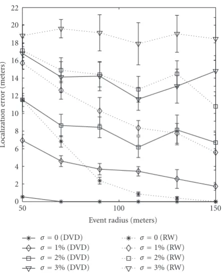
The lower localization error of CoE in DVD than in RW (Figure 19) is due to more number of packets arriving at the
BS from the event region (Section 5.2), which improves the
Least Squares estimation (forσ >0) or trilateration (forσ =
0) accuracy. A similar trend is observed for allσ andRe as
shown inFigure 19.
0.05
Event radius (meters)
σ=1% (DVD) Figure20: Sensitivity of Packet loss for DVD and RW.
Packet loss ratio has been defined as the Number
of packets dropped while relaying/Total Number of packets to be relayed. Figure 20 shows a comparable packet loss performance of both protocols. The packet loss ratio of RW remains constant for all event radii. The packet loss ratio of DVD drops with increase in event radius as the number of packets to be relayed is enhanced significantly with increase
in event radius (Figure 18).
The average number of hops are obtained considering only those packets that reach the BS successfully. Both DVD
and RW, asσ increases, packets relayed over more number
of hops are likely to be dropped. This lowers the average number of hops. DVD has a lower average number of hops
than RW, as seen in Figure 21. This is because, the relay
node chosen as the node with minimum waiting time at each hop in DVD, is more likely to be closer to the BS than the
relay node chosen by RW, as seen in Figures15and16and
explained inSection 5.1.
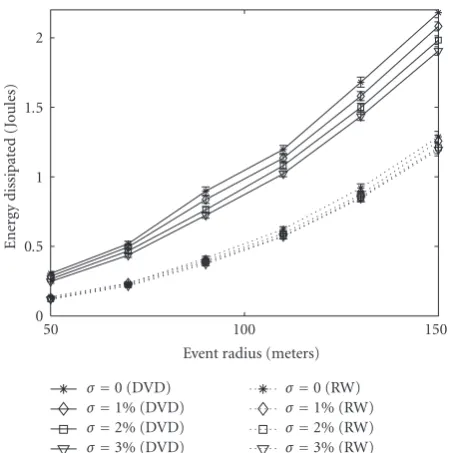
In both DVD and RW, the energy dissipated in the
network increases with event radius (Figure 22). However,
due to more number of packets to be relayed in DVD (Figure 18), the energy dissipated is higher than in RW. Also, the number of hops in RW is more than in DVD, resulting in
higher energy efficiency. In both cases, the energy dissipated
decreases with increase in perturbation as fewer number of
packets get effectively relayed in the network, due to higher
packet loss.
End-to-end delay has been computed only for data that successfully reaches the BS. The average delay is lower in
3
Event radius (meters)
σ=0 (DVD)
Figure21: Sensitivity of Average number of hops for DVD and RW.
0
Event radius (meters)
σ=0 (DVD)
Figure22: Sensitivity of Energy dissipated in the network for DVD and RW.
and lower waiting times (Section 4). Both for DVD and RW,
delay decreases with increase in perturbation (Figure 23).
This is because, packet losses are higher and packets located farther from the BS do not get relayed successfully.
The 95% confidence intervals show that DVD consis-tently outperforms RW in terms of localization accuracy and
2
Event radius (meters)
σ=0 (DVD)
Figure23: Sensitivity of end-to-end delay for DVD and RW.
end-to-end delay, however with a higher energy dissipation, for all event radii and perturbation ratios. For both protocols,
the confidence interval for average packet losses (Figure 20)
and average localization error (Figure 19) increases with
increasing σ, indicating a larger variance in performance
at higher perturbations. The small values of confidence intervals for energy dissipated, delay and average number of hops validate the robustness in the average performances of both protocols.
Figure 24shows the performance of a centralized scheme (Cellular Sensor Networks without multihop). As expected, the end-to-end delay is significantly lower than that of DVD while the localization error performance is comparable to that of DVD and slightly better at high event radii. The low end-to-end delay is due to single-hop transmission of sensed
data fromevent nodesto the BS. The large number of packets
generated from event region (Figure 18) is responsible for
the lower localization error of the centralized scheme, especially at high event radii. Packet losses are however high in the network due to long range transmissions. This limits the localization error performance especially at lower event radii where fewer number of nodes sense the event. More importantly, there is a significant increase in energy dissipated and possible congestion due to more number of packets transmitted in single hop from the event region (Figure 18).
0
Event radius (meters) (a)
Event radius (meters) (b)
Event radius (meters)
σ=0
Event radius (meters)
σ=0
σ=1%
σ=2%
σ=3% (d)
Figure24: Sensitivity Analysis of Packet loss ratio, Event Localization error, Energy dissipation, and average End-to-end delay for Centralized data aggregation.
Sensor Network (MCSN) with a distributed approach would be favorable compared to the Centralized approach. With respect to the existing RW protocol, the distributed waiting time based DVD protocol is more appealing due to its better event localization and delay performance for the moving event localization application of an MCSN.
7. Some Recent Works in
Cellular Sensor Networks
Urban, mobile, participatory, or people-centric sensingis being widely popularized as a technology which can bring about changes in people’s lives in a direct and profound manner,
[1, 2, 27, 28]. There are a large number of research and
development, academic and governmental partnerships, that
are attempting to makeurban sensing usingCellular Sensor
Networks, a tool for social change. Here, we have attempted
to include as many references as we can onCellular Sensor
Networks. For instance, in Accra, Ghana, pollution data was captured, throughout the day by GPS-supported Carbon monoxide sensor kits carried by taxi drivers and students
[29–31]. Ten other cases where cell phones contribute
to assistance in the areas of public health, security and
environmental conservation have been presented in [29].
TheUrban Sensing group atUCLA, [32], works on a large number of areas like public health, community cultural expression and well-being, environmental monitoring and
urban planning. TheMobile Millenniumproject uses
posi-tioning data from GPS-enabled cell phones mounted on
vehicles, to get real-time traffic information [5]. In [33],
a system, UbiFit garden, has been developed for people to
monitor lifestyle and to encourage physical activity. In [4],
projects ranging from personal sensing systems to sensing
terrain are under research, while [34] studies the real-time
movement patterns in Rome. Various underlying issues in
the development ofCellular Sensor Networksare discussed
for accessing the data from the sensors in a robust way, yet hiding the complexities underlying embedded mobile phone environment. Tackling security-related issues is considered
in [36], while [37] proposes a continuous query-processing
system for intermittently connected mobile sensor networks.
Handling of spatio-temporal queries efficiently from the
sen-sors is described in [38]. Data inferencing using cooperative
techniques to overcome device heterogeneity is considered in
[39].
8. Concluding Remarks
The main contribution of the paper is the Distributed Velocity-Dependent (DVD) waiting time based protocol for Multihop Cellular Sensor Networks (MCSNs). DVD exploits the Random Waypoint (RWP) distribution of cell phone users and is considered here for a moving event localization application. In this paper, the time-stationary probability density function (pdf) of waiting time in DVD has been derived. An analysis of the spatial distribution of waiting time, coupled with the inferences drawn from the pdf of the waiting time, validate the simulation results. Extensive simulations, carried out with perturbations in location, velocity and measured intensity, show that with or without perturbations, the proposed DVD protocol performs better than RW in terms of event localization and delay. Further, DVD based MCSN has a comparable event localization performance and significantly lower energy dissipation than the existing Centralized Cellular Sensor Network. We shall be considering the problem of localizing multiple events and overlap of event regions for possible extension of the proposed protocol.
Acknowledgments
This work is supported by DST under the IU-ATC (India-UK Advanced Technology Center) sponsored project on “Per-vasive Sensor Environments”. The first author acknowledges the TCS Research Fellowship for her Ph.D..
References
[1] A. Kansal, M. Goraczko, and F. Zhao, “Building a sensor network of mobile phones,” inProceedings of the 6th Interna-tional Symposium on Information Processing in Sensor Networks (IPSN ’07), pp. 547–548, Cambridge, Mass, USA, April 2007. [2] T. Abdelzaher, Y. Anokwa, P. Boda, et al., “Mobiscopes for
human spaces,”IEEE Pervasive Computing, vol. 6, no. 2, pp. 20–29, 2007.
[3] R. J. Honicky, “N-SMARTS: networked suite of mobile atmospheric real-time sensors,” Department of Computer Science, UC Berkely, 2008, http://www.eecs.berkeley.edu/∼ honicky/nsmarts/.
[4] MetroSense, “Tracking mobile events with mobile sensors,” MetroSense, Dartmouth, Mass, USA, 2008,http://metrosense .cs.dartmouth.edu/projects.html.
[5] M. Millenium, “Mobile millenium: using cell phones as mobile traffic sensors,” UC Berkeley College of Enginerring, CCIT, Caltrans, DOT, Nokia, NAVTEQ, 2008,http://traffic. .berkeley.edu/theproject.html.
[6] A. A. Somasundara, A. Kansal, D. D. Jea, D. Estrin, and M. B. Srivastava, “Controllably mobile infrastructure for low energy embedded networks,”IEEE Transactions on Mobile Computing, vol. 5, no. 8, pp. 958–972, 2006.
[7] M. Zhang, X. Du, and K. Nygard, “Improving coverage performance in sensor networks by using mobile sensors,” in
Proceedings of the IEEE Military Communications Conference (MILCOM ’05), Atlatnic City, NJ, USA, October 2005. [8] Y.-D. Lin and Y.-C. Hsu, “Multihop cellular: a new architecture
for wireless communications,” in Proceedings of the 19th Annual Joint Conference of the IEEE Computer and Commu-nications Societies (INFOCOM ’00), vol. 3, pp. 1273–1282, March 2000.
[9] G. Kannan, S. N. Merchant, and U. B. Desai, “Cross layer routing for multihop cellular networks,” in Proceedings of the 21st International Conference on Advanced Information Networking and Applications Workshops (AINAW ’07), vol. 1, pp. 165–170, May 2007.
[10] F. Bouhafs, M. Merabti, and H. Mokhtar, “Mobile event mon-itoring protocol for wireless sensor networks,” inProceedings of the 21st International Conference on Advanced Information Networking and Applications Workshops (AINAW ’07), vol. 2, pp. 864–869, IEEE Computer Society, Washington, DC, USA, 2007.
[11] W. Zhang and G. Cao, “DCTC: dynamic convoy tree-based collaboration for target tracking in sensor networks,” IEEE Transactions on Wireless Communications, vol. 3, no. 5, pp. 1689–1701, 2004.
[12] K.-W. Fan, S. Liu, and P. Sinha, “Structure-free data aggre-gation in sensor networks,” IEEE Transactions on Mobile Computing, vol. 6, no. 8, pp. 929–942, 2007.
[13] J.-Y. Le Boudec and M. Vojnovi´c, “Perfect simulation and stationarity of a class of mobility models,” inProceedings of the 24th Annual Joint Conference of the IEEE Computer and Communications Societies (INFOCOM ’05), vol. 4, pp. 2743– 2754, Miami, Fla, USA, March 2005.
[14] D. Chander, B. Jagyasi, U. B. Desai, and S. N. Merchant, “DVD based moving event localization in multihop cellular sensor networks,” inProceedings of the IEEE International Conference on Communications (ICC ’09), June 2009.
[15] V. I. Nikolaev and S. N. Yatsko, “A mathematical model, algo-rithm, and package of programs for simulation and prompt estimation of the atmospheric dispersion of radioactive pollu-tants,”Journal of Engineering Physics and Thermophysics, vol. 68, no. 3, pp. 385–394, 1995.
[16] D. Q. Zheng, J. K. C. Leung, B. Y. Lee, and H. Y. Lam, “Data assimilation in the atmospheric dispersion model for nuclear accident assessments,”Atmospheric Environment, vol. 41, no. 11, pp. 2438–2446, 2007.
[17] K. Kulkarni, S. Tilak, K. Chiu, and T. Fountain, “Engineer-ing challenges in build“Engineer-ing sensor networks for real-world applications,” inProceedings of the International Conference on Intelligent Sensors, Sensor Networks and Information Processing (ISSNIP ’07), pp. 693–698, Melbourne, Canada, December 2007.
[18] K. J. Kumar, B. S. Manoj, and C. S. R. Murthy, “RT-MuPAC: a new multi-power architecture for voice cellular networks,”
Computer Networks, vol. 47, no. 1, pp. 105–128, 2005. [19] W. C. Y. Lee,Wireless and Cellular Communications, McGraw
Hill, Boston, Mass, USA, 2005.
[21] J.-Y. L. Boudec, “Understanding the simulation of mobility models with palm calculus,” Tech. Rep. IC/2004/53, EPFL, Lausanne, Switzerland, 2004.
[22] C. Bettstetter and C. Wagner, “The spatial node distribution of the random waypoint mobility model,” in Mobile Ad-Hoc Netzwerke, 1. Deutscher Workshop ¨uber Mobile Ad-Ad-Hoc Netzwerke (WMAN ’02), pp. 41–58, GI, 2002.
[23] E. M. Royer, P. M. Melliar-Smith, and L. E. Moser, “An analysis of the optimum node density for ad hoc mobile networks,” inProceedings of the IEEE International Conference on Communications (ICC ’01), vol. 3, pp. 857–861, June 2001. [24] Y.-C. Hu and D. B. Johnson, “Caching strategies in on-demand routing protocols for wireless ad hoc networks,” inProceedings of the 6th Annual International Conference on Mobile Computing and Networking (MOBICOM ’00), pp. 231– 242, ACM, New York, NY, USA, 2000.
[25] C. Bettstetter, “Smooth is better than sharp: a random mobil-ity model for simulation of wireless networks,” inProceedings of the 4th ACM International Workshop on Modeling, Analysis and Simulation of Wireless and Mobile Systems, pp. 19–27, ACM, New York, NY, USA, 2001.
[26] X. Hong, M. Gerla, G. Pei, and C.-C. Chiang, “A group mobility model for ad hoc wireless networks,” inProceedings of the 2nd ACM International Workshop on Modeling, Analysis and Simulation of Wireless and Mobile Systems (MSWiM ’99), pp. 53–60, ACM, New York, NY, USA, 1999.
[27] J. Burke, D. Estrin, M. Hansen, et al., “Participatory sensing,” in Proceedings of the 4th ACM Conference on Embedded Networked Sensor Systems, November 2006.
[28] A. T. Campbell, S. B. Eisenman, N. D. Lane, E. Miluzzo, and R. A. Peterson, “People-centric urban sensing,” inProceedings of the 2nd Annual International Wireless Internet Conference (WICON ’06), Boston, Mass, USA, August 2006.
[29] S. Kinkade and K. Verclas, “Wireless technology for social change: trends in mobile use by NGOs,” United Nations Foundation, Vodafone Group Foundation, 2008, http://mobileactive.org/files/MobilizingSocialChange full. pdf.
[30] R. J. Honicky, E. A. Brewer, E. Paulos, and R. M. White, “N-SMARTS: networked suite of mobile atmospheric real-time sensors,” in Proceedings of the 2nd ACM Workshop on Networked Systems for Developing Regions (SIGCOMM ’08), pp. 25–29, Seattle, Wash, USA, 2008.
[31] E. Paulos, R. J. Honicky, and E. Goodman, “Sensing atmo-sphere,” inProceedings of the ACM Conference on Embedded Networked Sensor Systems (SenSys ’07), November 2007. [32] Urban Sensing, “Urban Sensing CENS/UCLA,” UCLA, 2008,
http://urban.cens.ucla.edu/vision.
[33] S. Consolvo, D. W. McDonald, T. Toscos, et al., “Activity sensing in the wild: a field trial of ubifit garden,” inProceedings of the 26th Annual Conference on Human Factors in Computing Systems (CHI ’08), pp. 1797–1806, April 2008.
[34] F. Calabrese, K. Kloeckl, and C. Ratti, “Wikicity: real-time urban environments,”IEEE Pervasive Computing, vol. 6, no. 3, pp. 52–53, 2007.
[35] A. Joki, J. A. Burke, and D. Estrin, “Campaignr: a framework for participatory data collection on mobile phones,” October 2007,http://escholarship.org/uc/item/8v01m8wj.
[36] C. Cornelius, A. Kapadia, D. Kotz, D. Peebles, M. Shin, and N. Triandopoulos, “AnonySense: privacy-aware people-centric sensing,” in Proceedings of the International Conference on Mobile Systems, Applications, and Services (MobiSys ’08), pp. 211–224, ACM Press, June 2008.
[37] Y. Zhang, B. Hull, I. Balakrishnan, and S. Madden, “ICEDB: intermittently-connected continuous query processing,” in
Proceedings of the 23rd International Conference on Data Engineering (ICDE ’07), pp. 166–175, Istanbul, Turkey, April 2007.
[38] Y. Ahmad and S. Nath, “COLR-tree: communication-efficient spatio-temporal indexing for a sensor data web portal,” in
Proceedings of the 24th IEEE International Conference on Data Engineering (ICDE ’08), pp. 784–793, April 2008.