Existence and stability analysis to a coupled system of implicit type impulsive boundary value problems of fractional order differential equations

(1)

R E S E A R C H

Open Access

Existence and stability analysis to a coupled

system of implicit type impulsive boundary

value problems of fractional-order

differential equations

Arshad Ali

1

_{, Kamal Shah}

1

_{, Fahd Jarad}

2*

_{, Vidushi Gupta}

3

_{and Thabet Abdeljawad}

4

*_{Correspondence:}

[email protected]

2_{Department of Mathematics,}

Faculty of Arts and Sciences, Çankaya University, Ankara, Turkey Full list of author information is available at the end of the article

Abstract

In this paper, we study a coupled system of implicit impulsive boundary value problems (IBVPs) of fractional diﬀerential equations (FODEs). We use the Schaefer ﬁxed point and Banach contraction theorems to obtain conditions for the existence and uniqueness of positive solutions. We discuss Hyers–Ulam (HU) type stability of the concerned solutions and provide an example for illustration of the obtained results.

Keywords: Coupled system; Arbitrary order diﬀerential equations; Impulsive conditions; Hyers–Ulam stability

1 Introduction

The fractional calculus is one of the most emerging areas of investigation. The fractional differential operators are used to model many physical phenomena in a much better form as compared to ordinary differential operators, which are local. Results derived by FDEs are much better and more accurate. For applications and details on fractional calculus, we refer the readers to [1–7]. Our work is concerned with implicit-type coupled systems of FODEs with impulsive conditions. The IFODEs are of high worth. Such equations arise in management sciences, business mathematics and other managerial sciences, and so on. Some physical phenomena have sudden changes and discontinuous jumps. To model such problems, we impose impulsive conditions on the differential equations at discontinuity points. For applications and recent work, we refer the readers to [8–29]. Coupled systems of FODEs have been studied extensively in the last few decades because in applied sci-ences, we deal with many physical problems that can be modeled via these systems. We would like to refer the readers to [30–36] and references therein.

Since in many situations, such as nonlinear analysis and optimization, finding the exact solution of differential equations is almost difficult or impossible, we consider approxi-mate solutions. It is important to note that only stable approxiapproxi-mate solutions are accept-able. Various approaches of stability analysis are adopted for this purpose. The HU-type stability concept has been considered in the numerous literature. The said stability analy-sis is an easy and simple way in this regard. This type concept of stability was formulated for the first time by Ulam [37], and then the next year it was elaborated by Hyers [38].

(2)

In the beginning, this concept was applied to ordinary diﬀerential equations and then ex-tended to FODEs. We refer the readers to [39–44]. Very recently, Ali et al. [45], studied the Ulam-type stability for coupled systems of nonlinear implicit fractional diﬀerential equations.

Motivated by the aforesaid work, in this paper, we investigate the following coupled system with impulsive and (m+ 2)-point boundary conditions:

⎧ ⎪ ⎪ ⎪ ⎪ ⎪ ⎪ ⎪ ⎪ ⎨ ⎪ ⎪ ⎪ ⎪ ⎪ ⎪ ⎪ ⎪ ⎩

C

0Dαtjξ(t) =Φ(t,μ(t),

C

0Dαtjξ(t)), t∈[0, 1],t=tj,j= 1, 2, . . . ,m,

C

0D

β

tiμ(t) =Ψ(t,ξ(t),

C

0D

β

tiμ(t)), t∈[0, 1],t=ti,i= 1, 2, . . . ,n,

ξ(0) =h(ξ), ξ(1) =g(ξ) and μ(0) =κ(μ), μ(1) =f(μ),

ξ(tj) =Ij(ξ(tj)), ξ(tj) =¯Ij(ξ(tj)), j= 1, 2, . . . ,m,

μ(ti) =Ii(μ(ti)), μ(ti) =I¯i(μ(ti)), i= 1, 2, . . . ,n,

(1)

where 1 <α,β≤2,Φ,Ψ : [0, 1]×R×R→R, andg,h;f,κ:C(J, R)→R are continuous functions deﬁned as

g(ξ) =

p

j=1

λjξ(ξj), h(ξ) =

p

j=1

λjξ(ηj),

f(μ) =

q

i=1

δiμ(ξi), κ(μ) =

q

i=1

δiμ(ηi),

ξi,ηi,ξj,ηj∈(0, 1) fori= 1, 2, . . . , q,j= 1, 2, . . . , p, and

ξ(tj) =ξ

t_j+–ξt_j–,

ξ(tj) =ξ

t_j+–ξt–_j,

μ(ti) =μ

t+_i–μt_i–,

μ(ti) =μ

t+_i–μt–_i.

The notationsξ(t+

j),μ(t+i) are right limits, andξ(tj–),μ(ti–) are left limits;Ij,¯Ij,Ii,I¯i: R→R

are continuous functions; and Dα

0+, D

β

0+are the Caputo-type fractional diﬀerential

opera-tors of orderαandβ, respectively.

For system (1), we discuss necessary and suﬃcient conditions for the existence and uniqueness of a positive solution by using the Schaefer ﬁxed point and Banach contraction theorems. Further, we investigate various kinds of HU and GHU stability.

2 Background materials and some auxiliary results

(3)

We deﬁne the spaces of all piecewise continuous functions

B1=PC(J, R) = ξ: J→R :j= 0, 1, 2, 3, . . . ,m,ξ

t+_j,ξt_j–andξt_j+,ξt–_j

exist forj= 0, 1, 2, 3, . . . ,m,

B2=PC(J, R) = μ: J→R :i= 0, 1, 2, 3, . . . ,n,μ

t+_i,μt–_iandμt_i+,μt_i–

exist fori= 0, 1, 2, 3, . . . ,n.

Clearly, B1and B2are Banach spaces under the normsξB1 =maxt∈J|ξ(t)|andμB2=

maxt∈J|μ(t)|, respectively. Their product B = B1×B2 is also a Banach space with norm

(ξ,μ)B=ξB1+μB2.

Deﬁnition 1([1]) The Caputo fractional derivative of a functionξ: (0,∞)→R is deﬁned by

C

0Dαtξ(t) =

t

0

(t–s)l–α–1

Γ(l–α) ξ

(l)₍_s₎_ds_,

wherel= [α] + 1, and [α] denotes the integer part of a real numberα.

Deﬁnition 2([4]) The Riemann–Liouville fractional integral of orderα∈R+of a function

ξ∈C((0,∞), R) is deﬁned as

0Iαtξ(t) =

1

Γ(α)

t

0

(t–s)α–1ξ(s)ds,

whereα> 0, andΓ is the gamma function, provided that the right-hand side is pointwise deﬁned on (0,∞).

Lemma 1([46]) Forα> 0,we have

0Iαt

_C 0D

α tξ(t)

=ξ(t) –

l–1

i=0

ξ(i)(0)

i! t

i_, _{where l}_{= [}_α_{] + 1.}

Lemma 2([46]) Forα> 0,the diﬀerential equationC_Dα

tξ(t) =x(t)has the following

solu-tion:

ξ(t) =0Iαtx(t) + l–1

i=0

ξ(i)(0)

i! t

i_,

where l= [α] + 1.

Theorem 1(Schaefer’s ﬁxed point theorem [47]) LetBbe a Banach space,and letT :

B→Bbe a completely continuous operator.If the setW ={ξ∈B: ξ=ηTξ, 0 <η< 1}is bounded,thenT has a ﬁxed point inB.

Deﬁnition 3([48]) The coupled system (1) is said to be HU stable if there exists Kα,β=

(4)

inequality

⎧ ⎪ ⎪ ⎪ ⎪ ⎪ ⎪ ⎪ ⎪ ⎪ ⎪ ⎪ ⎨ ⎪ ⎪ ⎪ ⎪ ⎪ ⎪ ⎪ ⎪ ⎪ ⎪ ⎪ ⎩

|C

0Dαtjξ(t) –Φ(t,μ(t),

C

0Dαtjξ(t))| ≤α, t∈J,

|ξ(tj) –Ij(ξ(tj))| ≤α, j= 1, 2, . . . ,m, |ξ(tj) –¯Ij(ξ(tj))| ≤α, j= 1, 2, . . . ,m; |C

0D

β

tiμ(t) –Ψ(t,ξ(t),

C

0D

β

tiμ(t))| ≤β, t∈J,

|μ(ti) –Ii(μ(ti))| ≤β, i= 1, 2, . . . ,n, |μ(ti) –¯Ii(μ(ti))| ≤β, i= 1, 2, . . . ,n,

(2)

there exists a unique solution (ϑ,σ)∈Bwith

(ξ,μ)(t) – (ϑ,σ)(t)≤Kα,β, t∈J. (3)

Deﬁnition 4([48]) The coupled system (1) is said to be GHU stable if there existsϕ∈

C(R+_{, R}+_{) with}_ϕ_{(0) = 0 such that, for any approximate solution (}_ξ_,_μ₎_∈_B_{of inequality (2),}

there exists a unique solution (ϑ,σ)∈Bof (1) satisfying

(ξ,μ)(t) – (ϑ,σ)(t)≤ϕ(), t∈J. (4)

DenoteΦα,β=max{Φα,Φβ} ∈C(J, R) > 0 and KΦα,Φβ=max{KΦα, KΦα}> 0.

Deﬁnition 5([48]) The coupled system (1) is said to be HU-Rassias stable with respect toΦα,βif there exists a constant KΦα,Φβsuch that, for some> 0 and for any approximate

solution (ξ,μ)∈Bof the inequalities

⎧ ⎨ ⎩

|C

0Dαtjξ(t) –Φ(t,μ(t),

C

0Dαtjξ(t))| ≤Φα(t)α, t∈J,

|C

0D

β

tiμ(t) –Ψ(t,ξ(t),

C

0D

β

tiμ(t))| ≤Φβ(t)β, t∈J,

(5)

there exists a unique solution (ϑ,σ)∈Bwith

(ξ,μ)(t) – (ϑ,σ)(t)≤KΦα,ΦβΦα,β, t∈J. (6)

Deﬁnition 6([48]) The coupled system (1) is said to be GHU-Rassias stable with respect

toΦα,βif there exists a constant KΦα,Φβsuch that, for any approximate solution (ξ,μ)∈B

of inequality (5), there exists a unique solution (ϑ,σ)∈Bof (1) satisfying

(ξ,μ)(t) – (ϑ,σ)(t)≤KΦα,ΦβΦα,β(t), t∈J. (7)

Remark1 We say that (ξ,μ)∈Bis a solution of the system of inequalities (2) if there exist functionsΘ,θ∈C(J, R) depending uponξ,μ, respectively, such that

(5)

(ii) and

In this section, we present our main results.

Theorem 2 The solution(ξ,μ)∈Bof the coupled system

is given by the integral equations

⎧

(6)

Corollary 1 In view of Theorem2,our coupled system(1)has the following solution:

tiμ(t)). To convert the considered problem into a ﬁxed point problem, we

(7)

Tβ(ξ,μ)(t) =tf(μ) + (1 –t)κ(μ) + k

i=1

(t–ti)I¯i

μ(ti)

–

k

i=1

t(1 –ti)I¯iμ(ti)

+

k

i=1 Ii

μ(ti)

–

k

i=1

tIiμ(ti) +

1

Γ(β)

t

ti

(t–s)β–1vξ,μ(s)ds

+ 1

Γ(β)

k

i=1 ti

ti–1

(ti–s)β–1vξ,μ(s)ds

+ 1

Γ(β– 1)

k

i=1

(t–ti)

ti

ti–1

– t

Γ(β)

k+1

i=1 ti

ti–1

– t

Γ(β– 1)

k

i=1

(1 –ti)

ti

ti–1

(ti–s)β–2vξ,μ(s)ds.

We obtain our results under the following assumptions:

(H1) for anyξ,μ∈C([0, 1], R), there existKg,Kh,Kf,Kκ> 0such that

g(ξ) –g(μ)_PC≤Kgξ–μPC, f(ξ) –f(μ)_PC≤Kfξ–μPC,

h(ξ) –h(μ)_PC≤Khξ–μPC, κ(ξ) –κ(μ)_PC≤Kκξ–μPC;

(H2) for all ξ,ξ¯,μ,μ¯ ∈R andt∈[0, 1]there existLΦ1> 0,0 <LΦ2< 1, LΨ1> 0, and

0 <LΨ2< 1such that

Φ(t,ξ,μ) –Φ(t,ξ¯,μ¯)≤LΦ1|ξ–ξ¯|+LΦ2|μ–μ¯|, Ψ(t,ξ,μ) –Ψ(t,ξ¯,μ¯)≤LΨ1|ξ–ξ¯|+LΨ2|μ–μ¯|;

(H3) there exist constantsA1,A2,A3andA4> 0such that, forξ,ξ¯,μ,μ¯ ∈R,

Ij(ξ) –Ij(ξ¯)≤A1|ξ–ξ¯|, I¯j(ξ) –¯Ij(ξ¯≤A2|ξ–ξ¯|, j= 1, 2, . . . ,m, Ii(μ) –Ii(μ¯)≤A3|μ–μ¯|, I¯i(μ) –¯Ii(μ¯≤A4|μ–μ¯|, i= 1, 2, . . . ,n;

(H4) there exist constantsk1,N1,k2,N2,k3,N3,k4,N4> 0such that

Ij(ξj)≤k1|ξ|+N1, I¯j(ξj)≤k2|ξ|+N2, j= 1, 2, . . . ,m, Ii(μi)≤k3|μ|+N3

and|¯Ii(μi)| ≤k4|μ|+N4,i= 1, 2, . . . ,n;

(H5) there exist constantsk5,k6,k7,k8such that g(ξ)≤k5, h(ξ)≤k6 for allξ∈C

[0, 1], R,

f(μ)≤k7κ(μ)≤k8

(8)

(H6) there exist some functionsp1,q1,r1andp2,q2,r2∈C(J, R+)such that, fort∈Jand

(μ,ξ)∈B, we have

Φt,μ(t),C₀Dα_t_jξ(t)≤p1(t) +q1(t)|μ|+r1(t)C0D

α tjξ(t)

withp1∗=supt∈J|p1(t)|,q1∗=supt∈J|q1(t)|, andr1∗=supt∈J|r1(t)|< 1and

Ψt,ξ(t),C₀Dα_t_jμ(t)≤p2(t) +q2(t)|μ|+r2(t)C0D

α tjξ(t),

withp2∗=supt∈J|p2(t)|,q2∗=supt∈J|q2(t)|, andr2∗=supt∈J|r2(t)|< 1.

Theorem 3 If assumptions(H1), (H2), (H3)and the inequality

ℵ=max(ℵ1,ℵ2) < 1 (11)

are satisﬁed,where

ℵ1=

Kg+Kh+ 2m(A1+A2) +

2LΦ1

1 –LΦ2

1 +m

Γ(α+ 1)+

m

Γ(α)

and

ℵ2=

Kf+Kκ+ 2n(A3+A4) +

2LΨ1

1 –LΨ2

1 +n

Γ(β+ 1)+

n

Γ(β)

,

then the coupled system(1)has a unique solution.

Proof Take (ξ,μ), (ξ¯,μ¯)∈Band consider

Tα(ξ,μ)(t) –Tα(ξ¯,μ¯)(t)

=

t

g(ξ) –g(ξ¯)+ (1 –t)h(ξ) –h(ξ¯)

+

k

j=1

(t–tj)I¯j

ξ(tj) –ξ¯(tj)

–

k

j=1

t(1 –tj)¯Ij

ξ(tj) –ξ¯(tj)

+

k

j=1 Ij

ξ(tj) –ξ¯(tj)

–

k

j=1 tIj

ξ(tj) –ξ¯(tj)

+ 1

Γ(α)

t

tj

(t–s)α–1uμ,ξ(s) –u¯μ,ξ(s)

ds

+ 1

Γ(α)

k

j=1 tj

tj–1

(tj–s)α–1

uμ,ξ(s) –u¯μ,ξ(s)

ds

+ 1

Γ(α– 1)

k

j=1

(t–tj)

tj

tj–1

(tj–s)α–2

ds

– t

Γ(α)

k+1

j=1 tj

tj–1

(tj–s)α–1

(9)

– t

Γ(α– 1)

k

j=1

(1 –tj)

tj

tj–1

(tj–s)α–2

ds

, (12)

which further means that

Tα(ξ,μ)(t) –Tα(ξ¯,μ¯)(t)

≤ |t|g(ξ) –g(ξ¯)+|1 –t|h(ξ) –h(ξ¯)+

k

j=1

|t–tj|

× ¯Ijξ(tj) –ξ¯(tj)+ k

j=1

|t||1 –tj|¯Ijξ(tj) –I¯jξ¯(tj)+ k

j=1

Ij(ξ(tj) –Ijξ¯(tj)

+

k

j=1

|t|Ijξ(tj) –Ijξ¯(tj)+

1

Γ(α)

t

tj

(t–s)α–1_u

μ,ξ(s) –u¯μ,ξ(s)ds

+ 1

Γ(α)

k

j=1 tj

tj–1

(tj–s)α–1uμ,ξ(s) –u¯μ,ξ(s)ds

+ 1

Γ(α– 1)

k

j=1

|t–tj| tj

tj–1

+ t

Γ(α)

k+1

j=1 tj

tj–1

+ t

Γ(α– 1)

k

j=1

|1 –tj| tj

tj–1

(tj–s)α–2|uμ,ξ(s) –u¯μ,ξ(s)|ds. (13)

By assumption (H2) we have

uμ,ξ(t) –u¯μ,ξ(t)=Φ

t,μ(t),uμ,ξ(t)

–Φt,μ¯(t),u¯μ,ξ(t)

≤LΦ1μ(t) –μ¯(t)+LΦ2uμ,ξ(t) –u¯μ,ξ(t)

= LΦ1 1 –LΦ2

μ(t) –μ¯(t). (14)

By assumptions (H1) and (H3) and inequality (14), taking the maximum over the interval J,

from inequality (13) we have

Tα(ξ,μ) –Tα(ξ¯,μ¯)_B

1

≤Kgξ–ξ¯B1+Khξ–ξ¯B1+mA2ξ–ξ¯B1

+mA2ξ–ξ¯B1+mA1ξ–ξ¯B1+mA1ξ–ξ¯B1+

LΦ1

(1 –LΦ2)Γ(α+ 1)

× μ–μ¯B1+

LΦ1m

(1 –LΦ2)Γ(α+ 1)

μ–μ¯B1+

LΦ1m

(1 –LΦ2)Γ(α)

μ–μ¯B1

+ LΦ1(m+ 1)

(1 –LΦ2)Γ(α+ 1)

μ–μ¯B1+

LΦ1m

(1 –LΦ2)Γ(α)

μ–μ¯B1

≤ ℵ1

ξ–ξ¯B1+μ–μ¯B1

(10)

where

ℵ1=

Kg+Kh+ 2m(A1+A2) +

2LΦ1

1 –LΦ2

1 +m

Γ(α+ 1)+

m

Γ(α)

.

Similarly, we have

Tβ(ξ,μ) –Tβ(ξ¯,μ¯)_B2≤ ℵ2

ξ–ξ¯B2+μ–μ¯B2

,

where

ℵ2=

Kf+Kκ+ 2n(A3+A4) +

2LΨ1

1 –LΨ2

1 +n

Γ(β+ 1)+

n

Γ(β)

,

from which we have

T(ξ,μ) –T(ξ¯,μ¯)_B≤ ℵ(ξ,μ) – (ξ¯,μ¯)_B,

whereℵ=max{ℵ1,ℵ2}. HenceTis a contraction, and therefore, by the Banach contraction

principle,Thas a unique ﬁxed point.

Theorem 4 If assumptions(H1)–(H6)hold,then the coupled system(1)has at least one solution.

Proof Here we use the Schaefer ﬁxed point theorem. We need to show that the operator

T has at least one ﬁxed point. There are several steps involved in this method.

Step1: We will show that the operatorT is continuous. Take a sequence (ξn,μn)→

(ξ,μ)∈B. For anyt∈J, we consider

Tα(ξn,μn)(t) –Tα(ξ,μ)(t)

≤ |t|g(ξn) –g(ξ)+|1 –t|h(ξn) –h(ξ)

+

k

j=1

|t–tj|¯Ij

ξn(tj)

–¯Ij

ξ(tj)+ k

j=1

|t||1 –tjI¯j

ξn(tj)

–¯Ij

ξ(tj)

+

k

j=1 Ij

ξn(tj)

–Ij

ξ(tj)+ k

j=1

|t|Ij(ξn(tj) –Ij

ξ(tj)

+ 1

Γ(α)

t

tj

(t–s)α–1_u

μ,ξ,n(s) –uμ,ξ(s)ds

+ 1

Γ(α)

k

j=1 tj

tj–1

(tj–s)α–1uμ,ξ,n(s) –uμ,ξ(s)ds

+ 1

Γ(α– 1)

k

j=1

(t–tj)

tj

tj–1

(tj–s)α–2uμ,ξ,n(s) –uμ,ξ(s)ds

+ |t|

Γ(α)

k+1

j=1 tj

tj–1

(11)

+ |t|

Γ(α– 1)

k

j=1

(1 –tj)

tj

tj–1

(tj–s)α–2uμ,ξ,n(s) –uμ,ξ(s)ds. (15)

By assumption (H2) we have

uμ,ξ,n(t) –uμ,ξ(t)=Φ

t,μn(t),uμ,ξ,n(t)

–Φt,μ(t),uμ,ξ(t)

≤LΦ1μn(t) –μ(t)+LΦ2uμ,ξ,n(t) –uμ,ξ(t)

= LΦ1 1 –LΦ2

μn(t) –μ(t). (16)

Sinceμn→μasn→ ∞, we have that, for eacht∈J,uμ,ξ,n(t)→uμ,ξ(t) asn→ ∞. Also, for eacht∈J,ξn(t)→ξ(t) asn→ ∞. Since every convergent sequence is bounded, there

exists a constant b such that|uμ,ξ,n(t)| ≤band|uμ,ξ(t)| ≤bfor eacht∈J. We have

(t–s)α–1_u

μ,ξ,n(s) –uμ,ξ(s)≤(t–s)α–1uμ,ξ,n(s)+uμ,ξ(s)

≤2b(t–s)α–1_,

(tj–s)α–1uμ,ξ,n(s) –uμ,ξ(s)≤(tj–s)α–1uμ,ξ,n(s)+uμ,ξ(s)

≤2b(tj–s)α–1,

(tj–s)α–2uμ,ξ,n(s) –uμ,ξ(s)≤(tj–s)α–2uμ,ξ,n(s)+uμ,ξ(s)

≤2b(tj–s)α–2.

Clearly, the functionss→2b(t–s)α–1_,_s_→_2b(_t

j–s)α–1, ands→2b(tj–s)α–2are integrable

on the interval [0, t]. Thus, by assumptions (H1)–(H3), inequality (16), and the Lebesgue

dominated convergence theorem, the right-hand side of inequality (15) goes to zero, that is,

Tα(ξn,μn)(t) –Tα(ξ,μ)(t)→0 asn→ ∞,

and thus

Tα(ξn,μn) –Tα(ξ,μ)→0 asn→ ∞.

This implies that the operatorTαis continuous. Similarly, we can show that the operator

Tβis continuous, so that the operatorT=

Tα Tβ

is continuous.

Step2: We deﬁne the setΩ={(ξ,μ)∈B:|(ξ,μ)| ≤with|ξ| ≤1and|μ| ≤2}, where

max{1,2}=. Fort∈J, we consider

Tα(ξ,μ)≤ |t|g(ξ)+|1 –t|h(ξ)+ k

j=1

|t–tj|¯Ijξ(tj)

+

k

j=1

|t||1 –tj|I¯jξ(tj)+ k

j=1

_I_j₍ξ(tj)+ k

j=1

|t|Ijξ(tj)

+ 1

Γ(α)

t

tj

(t–s)α–1uμ,ξ(s)ds+ k

j=1 tj

tj–1

(tj–s)α–1|uμ,ξ(s)|

(12)

+

k

j=1

|t–tj| tj

tj–1

(tj–s)α–2|uμ,ξ(s)| Γ(α– 1) ds+|t|

k+1

j=1 tj

tj–1

Γ(α) ds

+|t|

k

j=1

|1 –tj| tj

tj–1

Γ(α– 1) ds. (17)

By (H6) we have

uμ,ξ(t)≤p1(t) +q1(t)(ξ,μ)+r1(t)uμ,ξ(t) ≤p∗₁+q∗₁+r∗₁|ω|

= p

∗

1+q∗1

1 –r∗₁ =:χ. (18)

Thus by (H4), (H5), and (H6) from (17) we obtain the following result:

Tα(ξ,μ)_B1≤k5+k6+m(k21+N2) +m(k21+N2)

+m(k11+N1) +m(k11+N1) +

χ Γ(α+ 1)+

mχ Γ(α+ 1)

+ mχ

Γ(α)+

(m+ 1)χ Γ(α+ 1)+

mχ

Γ(α)=:ς1. (19)

Similarly, we can show that

Tβ(μ,ξ)_B

2≤ς2. (20)

Now ifmax(ς1,ς2) =ς, then we have

T(ξ,μ)_B≤ς.

This shows that bounded sets are mapped into bounded sets underT.

Step3: W will show thatTis equicontinuous. LetD⊆B. Then for (ξ,μ)∈Dandt1,t2∈J

such thatt1<t2, we consider

Tα(ξ,μ)(t2) –Tα(ξ,μ)(t1)

≤ |(t2–t1)

g(ξ) –g(ξ)– (t2–t1))

h(ξ) –h(ξ)

+

k

j=1

(t2–t1)¯Ij

ξ(tj) –ξ(tj)

–

k

j=1

(t2–t1)¯Ij

ξ(tj) –ξ(tj)

– (t2–t1)

× k

j=1 Ij

ξ(tj) –ξ(tj)

+

1

Γ(α)

t2

tj

(t2–s)α–1uμ,ξ(s)ds– 1

Γ(α)

t1

tj

(t1–s)α–1uμ,ξ(s)ds

+ 1

Γ(α– 1)

k

j=1

(t2–t1) tj

tj–1

(13)

–(t2–t1)

Γ(α)

k+1

j=1 tj

tj–1

(tj–s)α–1uμ,ξ(s)ds

– (t2–t1)

Γ(α– 1)

k

j=1

(1 –tj)

tj

tj–1

(tj–s)α–2uμ,ξ(s)ds|

≤ χ Γ(α)

t2

tj

(t2–s)α–1ds–

χ Γ(α)

t1

tj

(t1–s)α–1ds

+ kχ

Γ(α)(t2–t1) +

χ(k+ 1)(t2–t1)

Γ(α+ 1) +

kχ(t2–t1)

Γ(α) . (21)

We can see that the right-hand side of inequality (21) approaches to zero ast1→t2. Hence

Tα(ξ,μ)(t2) –Tα(ξ,μ)(t1)→0 ast1→t2.

Similarly, we can show that

Tβ(μ,ξ)(t2) –Tβ(μ,ξ)(t1)→0 ast1→t2.

Therefore by the Ascoli–Arzelà theorem the operatorsTα,Tβare completely continuous,

and consequentlyTis completely continuous.

Step4: Deﬁne the setZ={(ξ,μ)∈B: (ξ,μ) =δT(ξ,μ), 0 <δ< 1}. We will show thatZ

is bounded. If (ξ,μ)∈Z, then by deﬁnition (ξ,μ) =δT(ξ,μ). Hence for anyt∈J, we can

write

Tα(ξ,μ) =δ

tg(ξ) + (1 –t)h(ξ) +

k

j=1

(t–tj)I¯j

ξ(tj)

–

k

j=1

t(1 –tj)I¯jξ(tj)

+

k

j=1 Ij

ξ(tj)

–

k

j=1

tIjξ(tj) +

1

Γ(α)

t

tj

(t–s)α–1uμ,ξ(s)ds

+ 1

Γ(α)

k

j=1 tj

tj–1

+ 1

Γ(α– 1)

k

j=1

(t–tj)

tj

tj–1

– t

Γ(α)

k+1

j=1 tj

tj–1

– t

Γ(α– 1)

k

j=1

(1 –tj)

tj

tj–1

(14)

Taking the absolute values of both sides of (22) and using 0 <δ< 1, we have

Tα(ξ,μ)(t)≤ |t|g(ξ)+|1 –t|h(ξ)+ k

j=1

|t–tj|¯Ij

ξ(tj)

+

k

j=1

t(1 –tj)I¯jξ(tj)+ k

j=1 Ij

ξ(tj)+ k

j=1

|t|Ijξ(tj)

+ 1

Γ(α)

t

tj

(t–s)α–1uμ,ξ(s)ds

+ 1

Γ(α)

k

j=1 tj

tj–1

+ 1

Γ(α– 1)

k

j=1

(t–tj)

tj

tj–1

+ |t|

Γ(α)

k+1

j=1 tj

tj–1

+ |t|

Γ(α– 1)

k

j=1

(1 –tj)

tj

tj–1

(tj–s)α–2uμ,ξ(s)ds. (23)

From inequalities (18) and (19) we have

_T_α(ξ,μ)_B

1 ≤k5+k6+m(k21+N2) +m(k21+N2)

+m(k11+N1) +m(k11+N1) +

χ Γ(α+ 1)

+ mχ

Γ(α+ 1)+

mχ Γ(α)+

(m+ 1)χ Γ(α+ 1)+

mχ

Γ(α)=:ς1. (24)

Similarly, we can obtain

Tβ(μ,ξ)_B

2≤ς2. (25)

From (24) and (25) we have

Tα(ξ,μ)_B≤ς,

whereς=max(ς1,ς2). Thus the setSis bounded, and hence, by the Schaefer ﬁxed point

Theorem,Thas at least one ﬁxed point. Consequently, the considered coupled system (1)

has at least one solution.

4 Stability analysis

Theorem 5 If assumptions(H1)–(H3)and inequalities(11)are satisﬁed and if = 1 –

ℵ1ℵ2

(15)

Proof Let (ξ,μ)∈Λbe an approximate solution of inequality (2), and let (ϑ,σ)∈Λbe the

unique solution of the coupled system given by

⎧

By Remark1we have

⎧

By Corollary1the solution of problem (27) is

(16)

(17)

and

μ–σB2–

ℵ2

1 –ℵ2

ξ–ϑB2≤

2(4n+ 1) 1 –ℵ2

β,

respectively. Let2(4_1–m_ℵ+1)

1 = Cαand 2(4n+1)

1–ℵ2 = Cβ. Then the last two inequalities can be written

in matrix form as

1 – ℵ1

1–ℵ1

– ℵ2 1–ℵ2 1

ξ–ϑB1

μ–σB2

≤

Cαα Cββ

,

which yields

ξ–ϑB1

μ–σB2

≤

1

ℵ1

(1–ℵ1)

ℵ2

(1–ℵ2) 1

Cαα Cββ

, (31)

where

= 1 – ℵ1ℵ2

(1 –ℵ1)(1 –ℵ2)

> 0.

From system (31) we have

ξ–ϑB1 ≤

Cαα

+

ℵ1Cββ (1 –ℵ1)

,

μ–σB2 ≤

Cββ

+

ℵ2Cαα (1 –ℵ2)

,

which imply that

ξ–ϑB1+μ–σB2≤

Cαα

+

Cββ

+

ℵ1Cββ (1 –ℵ1)

+ ℵ2Cαα

(1 –ℵ2)

.

Ifmax{α,β}=andCα+

Cβ

+

ℵ1Cβ (1–ℵ1)+

ℵ2Cα

(1–ℵ2)= Cα,β, then (ξ,μ) – (ϑ,σ)_B≤Cα,β.

This shows that system (1) is HU stable. Also, if

(ξ,μ) – (ϑ,σ)_B≤Cα,βϕ()

withϕ(0) = 0, then the solution of system (1) is GHU stable.

For the next result, we assume that

(H7) There exist two nondecreasing functionsγα,γβ∈C(J, R+)such that

0Iαtγα(t)≤L1γα(t) and 0Itβγβ(t)≤L2γβ(t), whereL1,L2> 0.

Theorem 6 If assumptions(H1)–(H3)and(H7)and inequalities(11)are satisﬁed and if

= 1 – ℵ1ℵ2

(18)

Proof We can obtain the result by using Deﬁnition5and performing the same procedure

as in Theorem5.

5 Example

To testify our results established in the previous section, we provide an adequate problem.

(19)

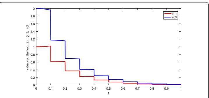
Figure 1Graphical representation of HU-stability results for Example1

we haveℵ1= 0.407 < 1 andℵ2= 0.467 < 1, that is,max(ℵ1,ℵ2) < 1. Therefore by Theorem3

the coupled system (32) has a unique solution. Also, = 1 – ℵ1ℵ2

(1–ℵ1)(1–ℵ2) = 0.8096104 >

0, and hence by Theorem5the coupled system (32) is HU stable and thus GHU stable. Similarly, we can verify the conditions of Theorems6and4. Next, we take the initial values for the required solutionξ= 1,μ= 2, and at the given fractional order the stability graph is given in Fig.1corresponding to the parametric values computed.

6 Conclusion

We successfully applied the Schaefer and Banach fixed point theorems to develop suffi-cient conditions for the existence of at least one solution and its uniqueness, respectively. Then we obtained some results for different kinds of HU stability. The whole analysis was demonstrated by an example.

Funding

The ﬁfth author would like to thank Prince Sultan University for funding this work through research group Nonlinear Analysis Methods in Applied Mathematics (NAMAM) group number RG-DES-2017-01-17.

Abbreviations

IBVP, implicit boundary value problem; FODEs, fractional-order diﬀerential equations; IFODEs, implicit fractional-order diﬀerential equations; HU, Hyers Ulam; GHU, generalized Hyers Ulam; GHUR, generalized Hyers Ulam Rassias.

Competing interests

The authors declare that they have no competing interests.

Authors’ contributions

All authors equally contributed to this paper and approved the ﬁnal version.

Author details

1_{Department of Mathematics, University of Malakand, Khyber Pakhtunkhwa, Pakistan.}2_{Department of Mathematics,}

Faculty of Arts and Sciences, Çankaya University, Ankara, Turkey.3_{Department of Mathematics, Indian Institute of}

Technology Guwahati, Guwahati, India.4_{Department of Mathematics and General Sciences, Prince Sultan University,}

Riyadh, Saudi Arabia.

Publisher’s Note

Springer Nature remains neutral with regard to jurisdictional claims in published maps and institutional aﬃliations.

(20)

References

1. Kilbas, A.A., Srivastava, H.M., Trujillo, J.J.: Theory and Applications of Fractional Diﬀerential Equations. North-Holland Mathematics Studies, vol. 204. Elsevier, Amsterdam (2006)

2. Kilbas, A.A., Marichev, O.I., Samko, S.G.: Fractional Integrals and Derivatives (Theory and Applications). Gordon and Breach, Switzerland (1993)

3. Miller, K.S., Ross, B.: An Introduction to the Fractional Calculus and Fractional Diﬀerential Equations. Wiley, New York (1993)

4. Podlubny, I.: Fractional Diﬀerential Equations. Academic Press, New York (1993) 5. Hilfer, R.: Applications of Fractional Calculus in Physics. World Scientiﬁc, Singapore (2000)

6. Rossikhin, Y.A., Shitikova, M.V.: Applications of fractional calculus to dynamic problems of linear and nonlinear hereditary mechanics of solids. Appl. Mech. Rev.50, 15–67 (1997)

7. Agarwal, R.P., Asma, Lupulescu, V., O’Regan, D.: Fractional semilinear equations with causal operators. Rev. R. Acad. Cienc. Exactas Fís. Nat., Ser. A Mat.111, 257–269 (2017)

8. Ali, A., Rabieib, F., Shah, K.: On Ulam’s type stability for a class of impulsive fractional diﬀerential equations with nonlinear integral boundary conditions. J. Nonlinear Sci. Appl.10, 4760–4775 (2017)

9. Shah, K., Ali, A., Bushnaq, S.: Hyers–Ulam stability analysis to implicit Cauchy problem of fractional diﬀerential equations with impulsive conditions. Math. Methods Appl. Sci.41, 1–15 (2018)

10. Ali, A., Shah, K., Baleanu, D.: Ulam stability results to a class of nonlinear implicit boundary value problems of impulsive fractional diﬀerential equations. Adv. Diﬀer. Equ.2019(5), 1 (2019)

11. Asma, Ali, A., Shah, K., Jarad, F.: Ulam–Hyers stability analysis to a class of nonlinear implicit impulsive fractional diﬀerential equations with three point boundary conditions. Adv. Diﬀer. Equ.2019(7), 1 (2019)

12. Wang, J., Zhou, Y., Fec, M.: Nonlinear impulsive problems for fractional diﬀerential equations and Ulam stability. Comput. Math. Appl.64(10), 3389–3405 (2012)

13. Wang, J., Feckan, M., Tian, Y.: Stability analysis for a general class of non-instantaneous impulsive diﬀerential equations. Mediterr. J. Math.14(2), 1–21 (2017)

14. Yang, D., Wang, J., O’Regan, D.: On the orbital Hausdorﬀ dependence of diﬀerential equations with non-instantaneous impulses. C. R. Acad. Sci. Paris, Ser. I356(2), 150–171 (2018)

15. Wang, J., Feckan, M., Zhou, Y.: Fractional order diﬀerential switched systems with coupled nonlocal initial and impulsive conditions. Bull. Sci. Math.141(7), 727–746 (2017)

16. Andronov, A., Witt, A., Haykin, S.: Oscillation Theory. Nauka, Moskow (1981)

17. Babitskii, V., Krupenin, V.: Vibration in Strongly Nonlinear Systems. Nauka, Moskow (1985)

18. Chua, L.O., Yang, L.: Cellular neural networks: applications. IEEE Trans. Circuits Syst.35, 1273–1290 (1988) 19. Chernousko, F., Akulenko, L., Sokolov, B.: Control of Oscillations. Nauka, Moskow (1980)

20. Popov, E.: The Dynamics of Automatic Control Systems. Gostehizdat, Moskow (1964)

21. Zavalishchin, S., Sesekin, A.: Impulsive Processes: Models and Applications. Nauka, Moskow (1991) 22. Abdeljawad, T., Jarad, F., Baleanu, D.: On the existence and the uniqueness theorem for fractional diﬀerential

equations with bounded delay within Caputo derivatives. Sci. China Ser. A, Math.51(10), 1775–1786 (2008) 23. Abdeljawad (Maraaba), T., Baleanu, D., Jarad, F.: Existence and uniqueness theorem for a class of delay diﬀerential

equations with left and right Caputo fractional derivatives. J. Math. Phys.49(8) (2008)

24. Alzabut, J., Abdeljawad, T.: A generalized discrete fractional Gronwall inequality and its application on the uniqueness of solution and its application on the uniqueness of solutions for nonlinear delay fractional diﬀerence system. Appl. Anal. Discrete Math.12, 036 (2018)

25. Abdeljawad, T., Alzabut, J., Baleanu, D.: A generalizedq-fractional Gronwall inequality and its applications to nonlinear delayq-fractional diﬀerence systems. J. Inequal. Appl.2016, 240 (2016)

26. Abdeljawad, T.: A Lyapunov type inequality for fractional operators with nonsingular Mittag-Leﬄer kernel. J. Inequal. Appl.2017, 130 (2017)

27. Abdeljawad, T., Alzabut, J.: On Riemann–Liouville fractionalq-diﬀerence equations and their application to retarded logistic type model. Math. Methods Appl. Sci.41(18), 8953–8962 (2018)

28. Abdeljawad, T., Al-Mdallal, Q.M.: Discrete Mittag-Leﬄer kernel type fractional diﬀerence initial value problems and Gronwall’s inequality. J. Comput. Appl. Math.339, 218–230 (2018)

29. Alzabut, J., Abdeljawad, T., Baleanu, D.: Nonlinear delay fractional diﬀerence equations with application on discrete fractional Lotka–Volterra model. J. Comput. Anal. Appl.25(5), 889–898 (2018)

30. Shah, K., Wang, J., Khalil, H., Khan, R.A.: Existence and numerical solutions of a coupled system of integral BVP for fractional diﬀerential equations. Adv. Diﬀer. Equ.2018, 149 (2018)

31. Ahmad, B., Nieto, J.J.: Existence results for a coupled system of nonlinear fractional diﬀerential equations with three-point boundary conditions. Comput. Math. Appl.58, 1838–1843 (2009)

32. Shah, K., Khan, R.A.: Existence and uniqueness of positive solutions to a coupled system of nonlinear fractional order diﬀerential equations with anti periodic boundary conditions. Diﬀer. Equ. Appl.7(2), 245–262 (2015)

33. Shah, K., Khan, R.A.: Multiple positive solutions to a coupled systems of nonlinear fractional diﬀerential equations. SpringerPlus5(1), 1–20 (2016)

34. Shah, K., Khalil, H., Khan, R.A.: Investigation of positive solution to a coupled system of impulsive boundary value problems for nonlinear fractional order diﬀerential equations. Chaos Solitons Fractals77, 240–246 (2015) 35. Su, X.: Boundary value problem for a coupled system of nonlinear fractional diﬀerential equations. Appl. Math. Lett.

22, 64–69 (2009)

36. Rehman, M., Khan, R.: A note on boundary value problems for a coupled system of fractional diﬀerential equations. Comput. Math. Appl.61, 2630–2637 (2011)

37. Ulam, S.M.: A Collection of the Mathematical Problems. Interscience, New York (1960)

38. Hyers, D.H.: On the stability of the linear functional equation. Proc. Natl. Acad. Sci. USA27(4), 222–224 (1941) 39. Hyers, D.H., Isac, G., Rassias, T.M.: Stability of Functional Equations in Several Variables. Birkhäuser, Boston (1998) 40. Ibrahim, R.W.: Generalized Ulam–Hyers stability for fractional differential equations. Int. J. Math.23(5) (2012) 9 pages 41. Jung, S.M.: Hyers–Ulam stability of linear differential equations of first order. Appl. Math. Lett.19, 854–858 (2006) 42. Jung, S.M.: On the Hyers–Ulam stability of functional equations that have the quadratic property. J. Math. Appl.222,

(21)

43. Li, T., Zada, A.: Connections between Hyers–Ulam stability and uniform exponential stability of discrete evolution families of bounded linear operators over Banach spaces. Adv. Diﬀer. Equ.2016(1), 1 (2016)

44. Li, T., Zada, A., Faisal, S.: Hyers–Ulam stability ofnth order linear diﬀerential equations. J. Nonlinear Sci. Appl.9, 2070–2075 (2016)

45. Ali, Z., Zada, A., Shah, K.: On Ulam’s Stability for a Coupled Systems of Nonlinear Implicit Fractional Diﬀerential Equations. Bull. Malays. Math. Sci. Soc.https://doi.org/10.1007/s40840-018-0625-x

46. Cabada, A., Wang, G.: Positive solutions of nonlinear fractional diﬀerential equations with integral boundary value conditions. J. Math. Anal. Appl.389(1), 403–411 (2013)

47. Granas, A., Dugundji, J.: Fixed Point Theory. Springer, New York (2003)