Development of a Synthetic Earth Gravity Model by 3D mass optimisation
based on forward modelling
J. J. Fellner, M. Kuhn, and W. E. Featherstone
Western Australian Centre for Geodesy and The Institute for Geoscience Research, Curtin University of Technology, GPO Box U1987, Perth, WA 6845, Australia
(Received March 2, 2010; Revised July 13, 2011; Accepted July 20, 2011; Online published March 2, 2012)
Several previous Synthetic Earth Gravity Model (SEGM) simulations are based on existing information about the Earth’s internal mass distribution. However, currently available information is insufficient to model the Earth’s anomalous gravity field on a global scale. The low-frequency information is missing when modelling only topography, bathymetry and crust (including the Mohoroviˇci´c discontinuity), but the inclusion of information on the mantle and core does not seem to significantly improve this situation. This paper presents a method to determine a more realistic SEGM by considering simulated 3D mass distributions within the upper mantle as a proxy for all unmodelled masses within the Earth. The aim is to improve an initial SEGM based on forward gravity modelling of the topography, bathymetry and crust such that the missing low-frequency information is now included. The simulated 3D mass distribution has been derived through an interactive and iterative mass model optimisation algorithm, which minimises geoid height differences with respect to a degree-360 spherical harmonic expansion of the EGM2008 global external gravity field model. We present the developed optimisation algorithm by applying it to the development of a global SEGM that gives a reasonably close fit to EGM2008, and certainly closer than a SEGM based only on the topography, bathymetry and crust.
Key words: Synthetic Earth Gravity Model (SEGM), global source model, 3D mass optimisation, forward gravity modelling.
1.
Introduction
As a precursor to the present study, Kuhn and
Featherstone (2005) demonstrated that information on the geometry and mass density within the Earth’s topography, bathymetry, crust and mantle allow for the computation of a coarse approximation of the Earth’s external gravity field (on a global scale) when compared to the ‘observed’ EGM96 global gravity field model (Lemoineet al., 1998). Although their SEGM generally showed similar patterns to EGM96, it lacked major information in the low-frequency band, suggesting insufficient mass-density information in the upper and middle mantle (∼60 km to∼1000 km depth). The geoid height differences between EGM96 and their SEGM ranged between±150 m on a global scale (most dif-ferences were below 50 m however), thus sometimes having larger magnitudes than the geoid signal itself. Furthermore, Kuhn and Featherstone (2005) showed that the inclusion of geophysical information on the Earth’s mantle (they used the S12WM13 seismic velocity anomalies model from Su et al.(1994)) did not provide significant improvement.
This paper presents a new way of determining a more re-alistic SEGM by using existing mass-density information within the Earth, supplemented by simulated mass-density distributions within the upper mantle. Such an improved
Copyright cThe Society of Geomagnetism and Earth, Planetary and Space Sci-ences (SGEPSS); The Seismological Society of Japan; The Volcanological Society of Japan; The Geodetic Society of Japan; The Japanese Society for Planetary Sci-ences; TERRAPUB.
doi:10.5047/eps.2011.07.012
SEGM—expressed here by the geoid heightN—represents a simulated but more realistic model of the Earth’s exter-nal gravity field. Therefore, such a model will be more suitable for performing Earth gravity-field related studies, such as the investigation of the behaviour of gravity inside the topographic masses. In this sudy, the simulated mass-density distribution is obtained from an iterative mass opti-misation algorithm (Fellneret al., 2010) based on forward gravity modelling. The main objective of a Synthetic [sim-ulated] Earth Gravity Model (SEGM) lies in its utility to validate and test existing and new methods in gravity field modelling (e.g. Featherstone, 1999; Kuhn and Featherstone, 2005; Baranet al., 2006; Tsoulis and Kuhn, 2007). The main advantage of a SEGM is that it generates exact grav-ity field quantities consistent with the used mass-densgrav-ity model. Any gravity field quantity can be calculated by applying forward gravity modelling techniques, enabling the prediction of how scientific experiments should perform and how well the Earth’s gravity field can be modelled.
Fundamentally, there are three classes of SEGMs (Pail, 1999): source models, effects models and hybrid source-effect models. All three are in common use, wheresource models mirror more or less realistic mass-density distri-butions within the Earth (e.g., Barthelmes and Dietrich, 1991; Vermeer, 1995; Claessenset al., 2001; ˚Agren, 2004; Kuhn and Featherstone, 2005), whereaseffects modelsrely entirely on observations of the Earth’s gravity field (e.g., Tziavos, 1996; Nov`aket al., 2001) such as from a combined Earth Gravity Model (EGM). Whileeffects modelsprovide
a global SEGM solely based on the new developed source mass model which results in a high-frequency SEGM after applying the Newton integral in the space domain (cf. Heck and Seitz, 2006).
2.
The Initial SEGM
Before explaining our iterative mass model optimisa-tion algorithm, we start with the construcoptimisa-tion of an initial SEGM based on existing information about the Earth’s to-pography, bathymetry and the crust-mantle boundary, the Mohoroviˇci´c discontinuity (Moho). The two global mod-els used for this initial SEGM are the min by 5-arc-min JGP95E digital elevation model (DEM; Lemoineet al., 1998, chap. 2) and the most recent 2-degree by 2-degree compilation of the Earth’s crustal mass distribution (thick-ness and mass heterogeneities) provided by CRUST 2.0, which is an updated version of CRUST 5.1 (Mooneyet al., 1998).
JGP95E classifies the global terrain into six different types (1: dry land below mean sea level (MSL), 2: lakes, 3: oceanic ice shelves, 4: oceans, 5: glacier ice, 6: dry land above MSL). These have been converted into equiva-lent rock heights (in spherical approximation, e.g., Rummel et al., 1988) with respect to a constant topographic mass-density of top = 2670 kg/m3 (Kuhn and Seitz, 2005).
While the total mass of each terrain type is conserved by the equivalent rock height approach, the geometry of the masses is changed, most prominently over the oceans (shal-lower with a density of 1030 kg/m3 for ocean water) and
ice-covered areas (lower elevation with a density of 927 kg/m3 for ice), while the global topography remains
un-changed.
While CRUST 2.0 provides the heights/depths of seven layers comprising ice, water, soft sediments, hard sedi-ments, upper crust, middle crust and lower crust, we only use the depths of the Moho. Inclusion of the remaining in-formation contained in CRUST 2.0 only changes the ini-tial SEGM minimally, but at the expense of increasing its complexity and hence the computation time. Mass anoma-lies at the Moho are defined with respect to a mean refer-ence sphere at a depth of 33 km. The numerical value for the density contrast at the Moho,M = 330 kg/m3, has
been taken from the Preliminary Reference Earth Model (PREM, Dziewonski and Anderson, 1981). Here, the av-erage Moho depths has been chosen about 10 km deeper than given by CRUST 2.0, which produces a SEGM that
sequently, the effect on the gravitational potential has been converted into the synthetic geoid height using Bruns’s for-mula (e.g., Heiskanen and Moritz, 1967, p. 293). Here the calculations of the gravitational potential is based on the principles described in Kuhn (2000, 2003), where the grav-itational effect of a spherical mass element is evaluated by that of a mass equal prism of the same height and centred at the same horizontal location. Here we use a spherical Earth model as the location of all masses are expressed with re-spect to spherical reference surfaces.
Figures 1 and 2 show the separate effects on the synthetic geoid induced by the combined topography and bathymetry and the mass anomalies at the Moho, respectively. Both effects show a similar spatial pattern but with opposite sign, indicating that—on a global scale—topography and bathymetry are largely compensated by the Moho mass anomalies. The combined effect of topography, bathymetry and Moho mass anomalies (cf. addition of Figs. 1 and 2) is illustrated in Fig. 3, which represents the synthetic geoid height of the initial SEGM.
In order to assess the quality of this initial SEGM, we compare the synthetic geoid heights (cf. Fig. 3) with that given by EGM2008, evaluated to degree and order 360. The geoid height differences, illustrated in Fig. 4, have a global range of about±220 m, which is about twice as large as the global geoid height range of EGM2008. This demonstrates the insufficient modelling of the Earth’s anomalous grav-ity field using only topography, bathymetry and Moho mass anomalies (see also Kuhn and Featherstone, 2005). How-ever, while the differences are large, the synthetic geoid al-ready shows some spatial patterns of the anomalous gravity field with generally larger ranges in magnitude (e.g., the geoid high over Iceland), but also fails to show other pat-terns (e.g., the geoid low over the Bay of Bengal).
Fig. 1. Effect on the synthetic geoid heightNcaused by JGP95E topog-raphy and bathymetry expressed in equivalent rock heights (Robinson Projection).
Fig. 2. Effect on the synthetic geoid heightNcaused by the Mohoroviˇci´c discontinuity in CRUST 2.0 (Robinson Projection).
Fig. 3. The initial SEGM derived from topography, bathymetry and Moho layer expressed in geoid heightN(Robinson Projection).
secondary importance as long as the final SEGM produces a gravity signal that is realistic. It may affect the convergence behaviour of our newly developed iterative mass optimisa-tion algorithm, explained in the next secoptimisa-tion.
Fig. 4. Difference between the synthetic geoid heights of the initial SEGM and EGM2008 (Robinson Projection). Note the larger differences coin-cide with some of the major plate boundaries (e.g., the mid-Atlantic ridge).
3.
Iterative Mass Model Optimisations
In this section, we present an iterative mass model opti-misation algorithm able to simulate mass distributions that create a gravity signal consistent with that of a given EGM (i.e., to be consistent with observations). While the optimi-sation algorithm can be applied for any gravity field func-tional, here we only explain it in terms of the geoid height N. In summary, the optimisation algorithm tries to improve a simulated mass distribution such that the generated syn-thetic geoid heights produce minimum differences to that of the EGM. As will be explained below, this has to be done in an iterative manner. In essence, the iterative mass opti-mation algorithm tries to fit a source model SEGM to an effects model SEGM given by the EGM.
Based on the sign and magnitude of the geoid height dif-ferences, it is possible to asses the simulated mass model. In order to do so in a numerically efficient way, we exploit the inverse property of Newton’s law of gravitation that a gravity signal diminishes with distance from the source masses. Therefore, as a first approximation, we assume that a particular geoid height difference is generated by insuf-ficient mass modelling in its near vicinity. We therefore assume that the simulated mass model, the synthetic geoid heights and the EGM-induced geoid heights are all given on co-located geographic grids with the same resolution, thus there are as many mass elements (here prisms) as geoid heights.
Fig. 5. Layout of the iterative mass model optimisation algorithm.
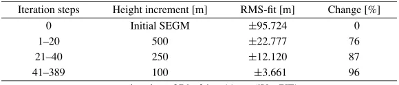
Table 1. Layout of the optimisation and convergence behaviour expressed by the overall RMS-fit. Iteration steps Height increment [m] RMS-fit [m] Change [%]
0 Initial SEGM ±95.724 0
1–20 500 ±22.777 76
21–40 250 ±12.120 87
41–389 100 ±3.661 96
processing time: 37 h: 24 m 11 sec (iVec/XE).
In order to start the iterative optimisation loop (step 1 in Fig. 5), an initial mass model and the geoid height dif-ferences have to be calculated. This is the initial SEGM constructed in Section 2. However, if no prior informa-tion is available, the iterainforma-tion could start with a “zero” mass model, thus the initial geoid height differences are identical to the EGM-induced geoid heights. In step 1, all mass ele-ments are adjusted based on the sign and magnitude of the co-located geoid height differences. This means masses are added/removed where the SEGM-induced geoid heights are too small/large compared to EGM2008.
In each iteration step, the mass elements are adjusted through their respective heights as long as the co-located geoid heigh difference exceeds a pre-set threshold (i.e., preference is given to the larger differences). Here the heights are changed by constant increments with larger in-crements used at the early stages of the iteration and smaller increments at later stages. Refer to Table 1 in chapter 4 for a choice of height increments used to derive the SEGM.
Based on the adjusted mass elements in step 2, the gravi-tational potential of the new mass model is derived and con-verted into synthetic geoid height changes in step 3. The result is superimposed with any prior information such as an initial SEGM in step 4 in order to obtain the new (im-proved) synthetic geoid height. Finally, the synthetic geoid height is compared to the EGM2008-induced geoid height (or any other geoid model, e.g., from GPS-levelling) and new geoid height differences are obtained. At this stage, the overall quality of the new mass model can be assessed. The RMS value of all differences (RMS-fit) is used and the iterative loop is repeated until the RMS-fit is less than a user-specified threshold. Furthermore, to avoid
unrealisti-clly large mass anomalies, their maximum extension is also limited by a user-defined threshold.
Instead of using only one mass model, the above optimi-sation algorithm can also be used to sequentially optimise a series of mass models (e.g., at different locations/depths). For example, the layered structure of the Earth’s interior can be modelled by a series of mass layers at different depths. Based on the layout of the optimisation algorithm, this has to be done sequentially, i.e., one mass layer at a time, and subsequently the information of a previously op-timised mass layer is introduced as prior information for the optimisation of the next layer. A possible strategy could be to model long-wavelength constituents first with deeper-seated masses, followed by the modelling of shorter-wavelength constituents with shallower masses.
4.
The Optimised SEGM
In order to demonstrate the performance of the iterative mass model algorithm described in Section 3, it has been applied to the initial SEGM from Section 2 with the aim of reducing the remaining geoid height differences (cf. Fig. 4). The iteration starts with prior information from the initial SEGM. In this study, we assume an additional mass layer located at the mean depth of 220 km (the Lehmann discon-tinuity), which also corresponds to one of the mantle tran-sition zones (Deuss and Woodhouse, 2004). Anomalous masses are added above or below the mean reference depth of 220 km corresponding to positive and negative mass anomalies, respectively. According to PREM (Dziewonski and Anderson, 1981), the constant mass-density contrast of 220 = 180 kg/m3 has been applied to all mass
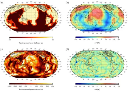
Fig. 6. (a) Simulated mass layer after the first iteration step with a height increment of 500 m. (b) Difference between the synthetic geoid heights of the optimised SEGM and EGM2008 after the first iteration step. RMS value:±87 m. (c) Simulated mass layer after the 100th iteration step with a height increment of 100 m. (d) Difference between the synthetic geoid heights of the optimised SEGM and EGM2008 after the 100th iteration step. RMS value:±5.4 m (Robinson projection).
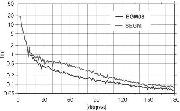
Fig. 8. Degree variances of the EGM2008- and SEGM-induced geoid heights. The spherical harmonic coeffients of the latter have been obtaind through a synthesis of SEGM-induced geoid heights illustrated in Fig. 7(c).
a 1-degree by 1-degree geographic grid. Finally, the con-stant height increments used in each iteration step are given in Table 1.
Before we analyse the SEGM, we illustrate how the al-gorithm optimises the mass layer. Figure 6(a) illustrates the initial mass layer with the according geoid height dif-ferences plotted in Fig. 6(b) after applying the effect of the simulated mass layer. A modest height increment of 500 m used in the first iteration steps led to considerable improve-ment (76%) with respect to the initial RMS-fit. The mass layer is further improved according the height increments given in Table 1. After the 100th iteration, the simulated mass layer shows a lot of fine structure (Fig. 6(c)) and the RMS-fit of the synthetic geoid height has improved by more than one order of magnitude. This is also demonstrated by the geoid height differences after the 100th iteration, illus-trated in Fig. 6(d), showing larger differences (e.g.>10 m) only at some isolated locations.
The final SEGM has been obtained after 389 iteration steps with the height increments used as given in Table 1. Figure 7(a) illustrates the optimised mass layer, which has a similar spatial pattern than that given after the 100th itera-tion step (cf. Fig. 6(c)). The effect of the optimised layer on the synthetic geoid height is illustrated in Fig. 7(b), which shows a similar spatial pattern to the geoid height differ-ences of the initial SEGM (cf. Fig. 4), now providing the missing (mostly low-frequency) information. This is con-firmed when superimposing the initial SEGM with the ef-fect of the optimised layer (i.e., adding Figs. 3 and 7(b)), resulting in the final SEGM.
The synthetic geoid height of the final SEGM is illus-trated in Fig. 7(c), which now has an almost identical spatial pattern than that of the ‘observed’ EGM2008 geoid (devel-oped up to degree and order 360). Also the amplitude range of−109 m to+92 m is very similar to that of the EGM2008 geoid (min:−106 m|max:+85 m). The oveall good fit of the final SEGM to EGM2008 is also shown by degree vari-ances that are almost identical for the first few degrees and of similar magnitude (cf. Fig. 8) for higher degrees. There-fore, the optimised SEGM may be used with some
confi-dence for Earth gravity field studies, and certainly more so than the model first presented by Kuhn and Featherstone (2005). However, it should be noted that the final SEGM always contains an omission error when obtained through comparison to a degree-360 truncated spherical harmonic expansion of EGM2008.
The geoid height differences between the final SEGM and EGM2008 are illustrated in Fig. 7(d). Although the differences range from −32 m to +52 m, larger differ-ences occur only in isolated locations (maximum values in the Andes region), which is also documented by the rather low RMS-fit of±3.6 m. The reason for the regional geoid anomaly in the Andes can be explained by sudden geoid height changes due to the presence of three differ-ent mass layers at three differdiffer-ent depth levels that com-bine to produce the total regional geoid anomaly (Bowin, 2000; Lucassenet al., 2001; Tassara et al., 2006). Based on the constant density assumption for this particular layer, it was not possible to model this geoid anomaly properly, although the modelled mass elements reach the maximum user-defined thickness of 100 kilometres in this area.
In addition a correlation between the simulated mass layer (cf. Fig. 7(a)) and geoid height differences (cf. Fig. 7(d)) can be noticed. Again this shows the inability of the final SEGM to replicate areas with sudden geoid height changes (most prominently in the Andes region). This mostly stems from the selected reference depth and resolution of the simulated mass distrubution and can fur-ther be improved by shallower and higher resolution masses that will also act to reduce the omission error.
5.
Conclusions and Future Work
the Earth’s observed gravity field, expressed here by the geoid height. Differences between the synthetic (simulated) geoid and that implied by EGM2008 have a RMS value of
±3.6 m, thus demonstrating that the developed SEGM is suitable for global Earth’s gravity field studies. However, the quality of localised studies depends on the fit as demon-strated by the larger geoid height differences over isolated areas (cf. Fig. 7(d)). Furthermore, the optimised mass layer should not be interpreted geophysically; it is only designed to replicate the external gravity field, so is subject to the problem of non-uniqueness of gravity inversion.
As shown for the final SEGM, the strategy allows for the development of mass distributions with an arbitrary geom-etry. This may be an advantage of using 3D mass elements (e.g., prisms) when compared to mass bodies of simpler ge-ometry (e.g., point masses or surface mass elements). How-ever, due to the more complex computation formulas, the use of prisms is limited when considering high-resolution applications over large areas because the computation time will become the major issue.
While the algorithm has been applied to a global SEGM with the aim of modelling mostly low-frequency con-stituents of the Earth’s gravity field, it can also be applied to any frequency band-width as well as to any computa-tion region (local, regional and global). Furthermore, the same procedure can be used with other more or less com-plex mass bodies. Once again, the limitations will be driven by the computer power available. However, with the in-creased availability of supercomputers, the boundary can be pushed to more complex applications.
Finally, it should be mentioned that the simulated mass model may be far from reality, thus any geophysical in-terpretation has to be handled with care considering all as-sumptions made. This is certainly the fact when only one major mass source is used (e.g., only one mass layer within the mantle). In this case, all other existing mass anomalies will be absorbed for in this mass source (the problem of non-uniqueness). However, this is not a problem when con-structing a SEGM. In order to improve the mass model fur-ther the developed procedure can be applied to practically an arbitrary number of mass sources (e.g., mass layers), thus it offers the possibility to incorporate other geophysical in-formation on the Earth’s interior. Therefore, there is still room to further improve the optimised SEGM with addi-tional known and simulated mass sources.
Acknowledgments. We would like to thank the EGM2008
De-velopment Team for providing the harmonic synth v2.f software. This work was supported by iVEC through the use of advanced computing resources provided by the ARRC facility located at Technology Park, Perth, Western Australia. JJF and MK acknowl-edge funding from Curtin University’s Institute for Geoscience Research (TIGeR). MK wishes to thank Curtin University of Tech-nology for support within his Research and Teaching Fellowship. WEF receives funding support under the Australian Research Council’s discovery projects funding scheme (grant DP0663020). All figures were produced using Generic Mapping Tools (GMT; Wessel and Smith, 1998). We would also like to thank the two reviewers for their time taken to assess this manuscript. This is TIGeR publication number 269.
References
˚
Agren, J., Regional geoid determination methods for the era of satel-lite gravimetry—Numerical investigations using synthetic Earth gravity models, Ph.D. thesis, Royal Institute of Technology (KTH), Department of Infrastructure, Stockholm, 2004.
Baran, I., M. Kuhn, S. J. Claessens, W. E. Featherstone, S. A. Holmes, and P. Van´ıˇcek, A synthetic Earth gravity model designed specifically for testing regional gravimetric geoid determination algorithms,J. Geod., 80, 2006.
Barthelmes, F. and R. Dietrich, Use of point masses on optimized posi-tions for the approximation of the gravity field, inDetermination of the Geoid: Present and Future, edited by R. H. Rapp and F. Sanso, 484 pp., Springer, 1991.
Bowin, C., Mass anomaly structure of the Earth,Rev. Geophys.,38, 355– 387, 2000.
Claessens, S. J., A synthetic Earth model analysis, implementation, valida-tion and applicavalida-tion, MSc. thesis, Delft University of Technology, Delft, Netherlands, 2002.
Claessens, S. J., W. E. Featherstone, and F. Barthelmes, Experiences with point-mass gravity field modelling in the Perth region,Geom. Res. Aust., 75, 53–86, 2001.
Deuss, A. and J. H. Woodhouse, The nature of the Lehmann discontinuity from its seismological Clapeyron slopes,Earth Planet. Sci. Lett.,225, 295–304, 2004.
Dziewonski, A. M. and D. L. Anderson, Preliminary Reference Earth Model,Phys. Earth Planet. Inter.,25, 297–356, 1981.
EGM2008, Earth Gravitational Model 2008, U.S. National Geospatial-Intelligence Agency (NGA), http://earthinfo.nga.mil/GandG/wgs84/ gravitymod/egm2008/index.html, 2008.
Featherstone, W. E., Progress report for IAG SSG3.177 syn-thetic modelling of the Earth’s gravity field, in International Association of Geodesy Travaux, edited by O. B. Anderson, http://www.gfy.ku.dk/˜iag/Travaux/ssg3177.htm, 1999.
Fellner, J. J., M. Kuhn, and W. E. Featherstone, Low-frequency geoid modelling based on 3D mass optimisation,Allgemeine Vermessungs Nachrichten,6, 220–226, 2010.
Haagmans, R., A synthetic Earth for use in geodesy,J. Geod.,74, 503–511, 2000.
Heck, B. and K. Seitz, A comparison of the tesseroid, prism and point mass approaches for mass reductions in gravity field modelling,J. Geod.,81, 121–136, 2006.
Heiskanen, W. and H. Moritz,Physical Geodesy, 364 pp., WH Freeman & Co, San Francisco, 1967.
Kuhn, M., Geoidbestimmung unter Verwendung verschiedener Dichtehy-pothesen, Ph.D. thesis, Deutsche Geod¨atische Kommission, Reihe C, No. 520, M¨unchen, Germany, 128 pp., 2000.
Kuhn, M., Geoid determination with density hypothesis from isostatic models and geological information,J. Geod.,77, 50–65, 2003. Kuhn, M. and W. E. Featherstone, Construction of a synthetic Earth
grav-ity model by forward gravgrav-ity modelling, inA Window on the Future of Geodesy, Volume 128 of International Association of Geodesy Sym-posia, edited by Springer Berlin Heidelberg, 350–355, 2005.
Kuhn, M. and K. Seitz, Comparison of Newton’s Integral in the Space and Frequency Domains, inA Window on the Future of Geodesy, Volume 128 of International Association of Geodesy Symposia, edited by Springer Berlin Heidelberg, 386–391, 2005.
Lemoine, F. G., S. C. Kenyon, J. K. Factor, R. G. Trimmer, N. K. Pavlis, D. S. Chinn, C. M. Cox, S. M. Klosko, S. B. Luthcke, M. H. Torrence, Y. M. Wang, R. G. Williamson, E. C. Pavlis, R. H. Rapp, and T. R. Olson, The development of the joint NASA GSFC and the National Imagery and Mapping Agency (NIMA) geopotential model EGM96, 575 pp., NASA/TP-1998-206861, National Aeronautics and Space Administra-tion, Greenbelt, USA, 1998.
Lucassen, F., R. Becchio, R. Harmon, S. Kasemann, G. Franz, R. Trumbull, H.-G. Wilke, R. L. Romer, and P. Dulski, Composition and density model of the continental crust at an active continental margin—the Central Andes between 21◦and 27◦S,Tectonophysics,341, 195–223, 2001.
Mooney, W., G. Laske, and T. Masters, Crust 5.1: A global crustal model at 5◦×5◦,J. Geophys. Res.,103, 727–747, 1998.
Nov`ak, P., P. Van´ıˇcek, M. Veronneau, S. Holmes, and W. E. Featherstone, On the accuracy of modified Stokes’s integration in high-frequency gravimetric geoid determination,J. Geod.,74, 644–654, 2001. Pail, R., Synthetic global gravity model for planetary bodies and