3GPP 3D MIMO channel model: a holistic implementation guideline for open source simulation tools

R E S E A R C H

Open Access

3GPP 3D MIMO channel model: a holistic

implementation guideline for open source

simulation tools

Fjolla Ademaj

, Martin Taranetz and Markus Rupp

Abstract

Massive MIMO and 3D beamforming have been identified as key technologies for future mobile cellular networks. Their investigation requires channel models that consider not only the azimuth- but also the elevation direction. Recently, the 3rd Generation Partnership Project (3GPP) has released a new 3D spatial channel model. It supports planar antenna arrays and enables to scrutinize concepts such as elevation beamforming and full dimension MIMO. A particular challenge is the practical implementation of the model. Dealing with enormous computational complexity requires to design a highly efficient approach. This paper provides a guideline for the practical implementation of the 3GPP 3D model into existing link- and system-level simulation tools. Considering the complexity of the model itself, our main focus is on computational efficiency. We present simulation examples using the proposed procedure with the Vienna LTE-A Downlink System Level Simulator. We measure simulation run times with respect to various network parameters. Our results allow to quantify the increase in complexity, when accounting for the elevation dimension. Moreover, they exhibit general trends when considering a large number of antenna elements per antenna array. We also draw a comparison with the WINNER channel model, which represents the most closely related channel model in 2D.

Keywords: 3GPP 3D channel model, System level simulations, Link level simulation, Open source, Interference channel, Elevation beamforming, Full-dimension MIMO, Vertical sectorization, Channel coefficient generation

1 Introduction

In the last decades, simulations have become a substantial tool for analyzing and designing wireless cellular commu-nication systems. As the systems themselves are growing in complexity, the effort of simulations becomes tremen-dous. Thus, the challenge is to keep the computational costs at a minimum while preserving accuracy. A com-monly employed solution is to divide the simulations into two stages or levels of abstraction, known as link-level and system-level [1]. Link-level simulations are used to assess the performance of the physical layer and those higher layer aspects directly related to the radio interface. Mostly, only a single radio link is evaluated, rarely some few users. System level simulations, on the other hand, aim to evaluate the performance of a whole network com-prising a substantial number of Evolved Node B (eNodeB)

*Correspondence: [email protected]

Christian Doppler Laboratory for Dependable Wireless Connectivity for the Society in Motion, TU Wien, Institute of Telecommunications, Gusshausstrasse 25/389, A-1040 Vienna, Austria

sectors and user equipments (UEs) [2, 3]. At the UEs, both the signals received from the serving as well as the inter-fering eNodeB sectors are modeled, taking into account large- as well as small-scale fading effects. Realistic mod-els for the small-scale effects, also known as channel models, impose a major challenge in describing wireless communications. Broadly speaking, channel models can be divided into two categories,deterministicand stochas-tic[4]. Deterministic models describe the channel for a specific propagation environment between eNodeB sec-tor and UE. This method can be tedious to evaluate and does not allow for general statements in an ensemble of environments. In stochastic models, the channel charac-teristics are condensed to a statistical description, e.g., the power delay profile (PDP) [5–7].

In order to close the gap between the two approaches, the 3rd Generation Partnership Project (3GPP) has intro-duced the Spatial Channel Model SCM [8]. Unlike tradi-tional channel models, it incorporates not only a random PDP but also a random angular profile (AP). The model

represents scatterers through statistical parameters with-out having a real physical location. The SCM belongs to the class ofgeometric stochasticmodel and separately defineslarge-scale parameters(e.g., shadow fading, delay spread, and angular spreads) and small-scale parame-ters(e.g., delays, cluster powers, and arrival- and depar-ture angles). Both parameter sets are randomly drawn from tabulated distributions. The large-scale parameters encompass the geometric positions of the eNodeB sec-tors and the UEs, respectively. Moreover, they are used to parameterize the statistics of the small scale parameters. The SCM model in [8] includes six different scenarios, each of them representing a unique environment. Initially, it was targeted for a bandwidth of 5 MHz and a carrier frequency of 2 GHz. Later, it was extended to theSpatial Channel Model Extended (SCME). The SCME follows the same procedure as the SCM, but supports bandwidths of up to 100 MHz and a frequency range of 2−6 GHz. In the course of the Wireless World Initiative New Radio (WIN-NER) projects, the model was extended for 15 different scenarios [9, 10], including urban-, rural-, and moving environments. The WINNER model is recommended as a baseline for evaluating radio interface technologies in the International Telecommunication Union - Radiocommu-nication Sector (ITU-R) [11].

The interest in 3-dimensional (3D) beamforming is greatly increasing in industry and standardization con-sortia, enabling concepts such as full dimension (FD)-multiple input (FD)-multiple output (MIMO) and vertical sectorization [12, 13]. Consequently, describing chan-nel characteristics in three dimensions, including both azimuth- and elevation angles is becoming indispensable. Recently, 3GPP introduced a new 3D SCM for Long Term Evolution-Advanced (LTE-A) in their recommendation TR 36.873 [14].

As of this writing, only a few simulation studies, includ-ing reports from the 3GPP TSG RAN WG1 meetinclud-ings, have been published, claiming the practical implementa-tion of the model [15, 16]. In [17], we have introduced the implementation and validation of the 3GPP 3D channel model in open source simulation tools, considering only the desired signal channels, while the interfering chan-nels are modeled by Rayleigh fading. In this contribution, we extend our approach considering also the interfering links to fade according to the 3GPP 3D channel model. We provide a complete guideline for the practical imple-mentation of the model. The MATLAB source code is openly available for download on our webpage under an academic, non commercial use license [18]. It is provided as a stand-alone package that is directly applicable for sys-tem level simulation tools and can straightforwardly be ported to link level. We strongly believe thatopen access

is a key prerequisite for reproducible simulation studies. Moreover, we have made an iteration of the model openly

available, with over 100 beta testers and an active online forum. We see it as the only way to ensure the quality of implementation. In this paper, we focus on downlink. According to [14], the channel can be applied for both up-and downlink. For this reason, the notionstransmitterand

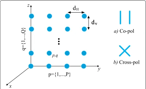
receiverinterchangeably refer to the antenna elements of the eNodeB sectors and the UEs, respectively. In practice, eNodeB sectors and UEs will be equipped with antenna arrays, each consisting of one or more antenna elements (conf. Fig. 2). Note that an eNodeB comprises a base band processing unit and can serve multiple sectors or cells.

This contribution outlines as follows. A brief descrip-tion of the 3GPP 3D channel model is provided in the beginning of Section 2, followed by a guideline for its com-putationally efficient implementation. In Section 3, the implementation is validated against results from the 3GPP standard with the Vienna LTE-A System Level Simulator. Moreover, simulation run time measurements are pro-vided with respect to various parameters that determine the network complexity. We also compare the 3GPP 3D model with the WINNER channel model. Section 4 out-lines challenges and new opportunities for investigations. Section 5 concludes the work.

2 3GPP 3D channel model in system level

simulator

2.1 3GPP 3D channel model

The 3GPP 3D channel model characterizes wireless com-munication channels of typical European cities. It is a 3D geometric stochastic model, describing the scatter-ing environment between eNodeB sector and UE in both azimuth and elevation dimensions. The scatterers are rep-resented by statistical parameters without having a real physical location. In 3GPP TR 36.873 [14], three scenar-ios, urban macro cell (UMa), urban micro cell (UMi), and UMa-high rise (UMa-H) are specified. They represent typical urban macro-cell and micro-cell environments. Both UMa and UMa-H scenarios, consider an sector antenna height of 25 m, thus surpassing the surround-ing buildsurround-ings. UMa-H also specifies such environments with one high-rise building per eNodeB sector. UMi, con-siders a sector antenna height of 10 m, lying below the rooftop level. All three environments are assumed to be densely populated with buildings and take into account both indoor- and outdoor UEs.

UE as well as the break point distance. The break point distance characterizes the gap between transmitter and receiver at which the Fresnel zone is barely broken for the first time [19]. For an indoor UE, LOS refers to the signal propagation outside the building in which the UE is located. For each UE location, large-scale parameters are generated according to its geographic position as well as the propagation conditions at this location. The large scale parameters incorporate shadow fading, the Ricean K-factor (only in the LOS case), delay spread, azimuth angle spread of departure- and arrival, as well as zenith angle spread of departure- and arrival.

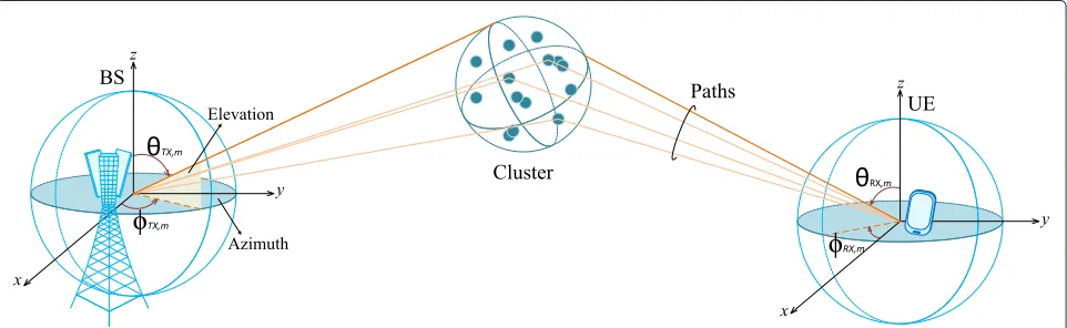
The small-scale parameters incorporate delays, clus-ter powers as well as angles of departure and -arrival in azimuth, and elevation direction, respectively. The model considersN clusters of scatterers, where each cluster is resolvable toMpaths. A simplified sketch of the model is given in Fig. 1. The channel coefficients are defined per clustern, sector antenna elementsand UE antenna elementuas patterns of the receive antenna elementuin the direction

of the spherical basis vectors,θˆin the zenith direction,φˆ in the azimuth direction. The expressionsFtx,s,θandFtx,s,φ

are field patterns of the transmit antenna element s in the direction ofθˆandφˆ, respectively. The departure- and arrival angels in zenith and azimuth direction are denoted withθ andφ, respectively. The termKn,mrepresents cross polarization power ratios for each path m and cluster

n, and _n,mAB are random initial phases for four different polarization combinations AB = {θθ,θφ,φθ,φφ}. The termsrˆrx,n,m andrˆtx,n,mare the receiver and transmitter spherical unit vectors expressed in Cartesian coordinates. They are defined as

The parametersd¯rx,uandd¯tx,sare the location vectors of receive and transmit antenna elements, respectively. Con-sidering an eNodeB sector with coordinatessx,sy,sz

, and a planar antenna array, the location vector per antenna element is ber of antenna elements and the element spacing in the horizontal direction, whileQanddV are the number of antenna elements and the element spacing in the verti-cal direction, respectively. The last component of (1),vn,m, represents the Doppler frequency component of the UE moving at velocity¯v. Further details on the calculation of the variables in (1) can be referred from [14].

2.2 Antenna modeling

The 3GPP 3D channel model enables to scrutinize 2-dimensional (2D) planar antenna arrays, also known as rectangular arrays. The antenna elements can either be

linearly polarized (co-pol) or cross prolarized (cross-pol), as shown in Fig. 2. In this regard, the model represents a compromise between practicality and precision as it does not include the mutual coupling effect as well as dif-ferent propagation effects of horizontally and vertically polarized waves. Our well-structured implementation will substantially facilitate the implementation of further tech-niques for modeling different polarization modes such as the one proposed in [20].

The antenna elements are equidistantly spaced in the

y- and thez-direction. For static electrical beam steering, also known aselectrical tilting, a complex weight is applied to each antenna element in the vertical direction. For an antenna element in theq-th row, it is given as

wq=

whereQrepresents the total number of antenna elements in the vertical direction andθetiltis the steering angle in

the vertical plane. Unlike the conventional approach of applying an array factor to the field pattern of a single ele-ment of a uniform antenna array, in the 3D model, the beamforming weights are applied to the channel coeffi-cients for each antenna element

channel coefficients. The index i indicates the eNodeB sectors, wherei=0 denotes the serving sectors, while the indicesi = {1, 2,. . .}refer to the interfering sectors. The termsPaandPbdenote the sets of antenna elements that belong to receive antenna port awith a ∈ {1,. . .,NRx}

and transmit antenna portbwithb∈ {1,. . .,NTx},

respec-tively. The terms ωu and ωs are complex weights that account for phase shifts as applied for static beamform-ing (e.g., electrical downtiltbeamform-ing), respectively. The relative

Fig. 2Geometry and polarization modes of a planar antenna array. The antenna elements in the horizontal and vertical directions are indexed bypandq, respectively

position of each element in the array is incorporated in the channel coefficients Hu,s,n(t), wherendenotes the clus-ter index,sanduare the eNodeB sector and UE antenna elements, respectively.

In the following, a detailed procedure on the implemen-tation of the model for simulations is provided.

2.3 Implementation in system-level

In this section, we describe the necessary steps to inte-grate the 3D channel model into an existing simulation tool. The target is to compute a NRx × NTx

MIMO-channel matrix H(t,f) for each sampling point on the time-frequency grid, whereNTxandNRxrefer to the

num-ber of transmit- and receive antenna ports, respectively. On link level, channel realizations are typically calculated per OFDM symbol and LTE-A subcarrier [21]. On system level, they are commonly generated per physical resource block (RB) and transmission time interval (TTI) [22].

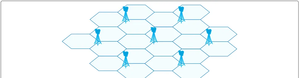
In the 3GPP 3D channel model, the channel coeffi-cients depend on the UE location in the 3D space and, thus, have to be calculated at runtime. The calculation complexity directly scales with the number of interfering channels. In view of this, a complexity reduction can be achieved by neglecting the contribution of those interfer-ers that have a received power below a certain threshold (e.g., the noise power). Consider a network scenario with hexagonally arranged macro-sites as illustrated in Fig. 3. The network comprises seven sites, each employing three eNodeB sectors. In each eNodeB sector, 50 UE are ran-domly distributed according to a uniform distribution. For a 4×4 MIMO configuration, the number of channel coef-ficients that needs to be generated in each time instant of the simulation is 1.41×108. Hence, in order to reduce complexity, the challenge is to perform computationally intensive tasksoff-lineoron demand, whenever possible.

We will follow the stepwise procedure as specified in ([14] Sec. 7.3) and implemented in [17] for the desired channel. This consists of 12 steps, which we will subse-quently denote as ’Step N’ with N∈ {1, . . , 12}, as illus-trated in Fig. 4. We will explain its expedient partition for implementation, and emphasize the additional steps for the interfering channels.

Fig. 3Hexagonal-grid macro-cell scenario with seven macro sites and 21 eNodeB sectors. This scenario is used in simulations throughout the paper

Different path loss models are applied for LOS, NLOS and, O-to-I, as defined in ([14] Tab. 7.2-1). The expe-rienced path loss is calculated in Step 3. In Step 4, the large-scale parameters are generated. The detailed proce-dure is described in ([10] Sec. 3.3.1). For each UE, a matrix of large scale parameters is generated as

LSP= ⎛ ⎜ ⎜ ⎜ ⎝

δ0,SK δ0,K δ0,DS δ0,ASD · · · δ0,ZSA

δ1,SK δ1,K δ1,DS δ1,ASD · · · δ1,ZSA

..

. ... ... ... . .. ... δi,SK δi,K δi,DS δi,ASD · · · δi,ZSA

⎞ ⎟ ⎟ ⎟

⎠, (6)

where the serving eNodeB sector is denoted by index 0 and the interfering eNodeB sectors are denoted by the indices i = {1,. . .,I}. In case the UE is not in LOS of BSi,δi,K =0. These tasks can be performed off-line, i.e.,

before entering the actual simulation loop. Moreover, they

can be carried out simultaneously for serving- and inter-fering eNodeB tors, allowing to employ, e.g., MATLAB’s parallel computing toolbox. Similar to the generation of the shadow fading, they have to be performed onlyonce per site.

[SSP]iThe next step is to generatesmall-scale param-etersfor desired and interfering signals. In the 3GPP 3D channel model, channel coefficientsHi,u,s,n(t) are deter-mined individually for each eNodeB sectori, each cluster

n, and each receiver- and transmitterantenna elementpair {u,s}, respectively. Similar to the implementation in [17], the calculation of Hi,u,s,n(t) requires to generate delays (Step 5), cluster powers (Step 6) as well as arrival- and departure angles for both azimuth and elevation (Step 7). After coupling the rays within a cluster (Step 8), cross polarization power ratios (XPRs), and random ini-tial phases are drawn (Step 9 and 10). Together with the calculation of the spherical unit vectors and the Doppler

frequency component (bothStep 11), all parameters men-tioned above are commonly applied to each antenna ele-ment pair{u,s}and thushave to be determined only once per antenna array and eNodeB sector. The Doppler com-ponent accounts for the time variance of the channel. The frequency selectivity is determined by the channel impulse responseHi,u,s,n(t) and the sampling frequency, which is directly related to the system bandwidth.

[CG]iAfter generating the channel coefficients for each antenna element pair {u,s}, the channel coefficients for an antenna array are combined according to the antenna element-to-port mapping given in Sec. 2.2. Then, the combined channel Hc_i,n(t), for each cluster nis sampled based on the delay tapsmdefined as

m= domain andτndenotes the actual delay of then-th clus-ter. The sampledNRx× NTx channel matrix is denoted

asHˆi,m(t), with an element

ˆ

Hi,m(t)

a,b, referring to the sampled channel coefficient for receive antenna port a

and transmit antenna port b, respectively. It is impor-tant to note that the model is designed such that the channel impulse response before sampling has unit sum power on average overt, i.e.,Etn|

Hc_i,n(t)_a,b|2=1, when assuming antenna elements with omni-directional

gain pattern and 0 dB gain, as well as an XPR of one. In order not to change the sum power after the sampling, we multiply the sampled channel coefficientsHˆi,m(t)

channel transfer function is obtained by performing a fast Fourier transform (FFT) over the sampled and normalized channel impulse response number of FFT samples which is the maximum number of delay tapsm. For example, assuming a transmission band-width of 10 MHz, according to [23], the sampling interval isTs=65 ns and the number of FFT samples is N=1024. Considering a UE with a fixed location in the 3D space, [SSP]i and[CG]i have to be carried out only in the first time instant of the simulation. Afterwards, the channel will remain static over time (no Doppler effect). If the UE moves at a certain speed, represented by the vector v∈R3, in principle,[SSP]iwould have to be performed at runtime in each time instant of the simulation. This also implies the generation of new clusters and random initial

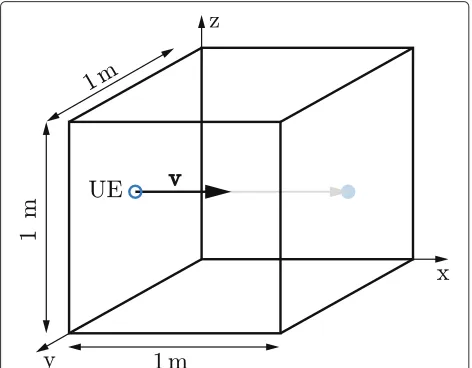
phases, i.e., a complete change of the multi-path propaga-tion environment. Thus, it is considered reasonable from a physical perspective (see, e.g., [10]) as well as in view of computational complexity to partition the scenario into equally sized cubes. As long as the UE resides within the same cube, it is assumed to experience the same path loss, shadow fading, propagation conditions (LOS/NLOS/O-to-I), and large scale parameters, as generated in [GP]. Then,[SSP]ihas to be carried out only once at the begin-ning of the simulation and each time the UE transfers to another cube. Assuming a spatial resolution of 1 m and a temporal resolution of 1 ms, referring to the length of one LTE sub-frame, also denoted as TTI, a UE moving atv =[ 27.78, 0, 0] m/s requires 36 ms to travel from one face of the cube to the other, as indicated in Fig. 5. In this case,[SSP]i is performed every 36 sub-frames. Within a cube, channel variations are caused by the slightly chang-ing angles of arrival and departure (and thus the antenna element field patterns) as well as the phase shift due to the Doppler effect. They can be incorporated into[CG]i thus yielding the only variable components that have to be recalculated in each time instant of the simulation. If the UE trace is known, e.g., in train and car sce-narios, the simulation complexity can be reduced even further. In such scenarios, the Doppler frequency com-ponent in (1) has to be calculated only in the first time instant of the simulation, and can be reused in subsequent time instances as long as the user stays within the same cube.

3 Simulation run times and throughput

performance evaluation

We now demonstrate the application of the proposed pro-cedure in an existing system level simulation tool. In [17], we have demonstrated the implementation of the 3GPP

3D model for the desired channel. We now extend this approach by also taking into account the interfering links. We integrate our code into the Vienna LTEA Downlink System Level Simulator (current version v1.8r1375) [22]. The simulator is implemented in object-oriented MAT-LAB and is made openly available for download under an academic, non-commercial use license. It is built accord-ing to the commonly employed structure for system level simulation tools (see, e.g., in [1, 24]), as illustrated in Fig. 6 and, thus, serves as a representative example. Its center-piece is thelink abstraction modelthat specifies the inter-action between link- and system level simulations [1, 22]. This structure is expected to persist in simulation tools for the fifth generation of mobile cellular networks (5G) [24]. The enhancements that were necessary to enable the 3GPP 3D channel model for desired and interfering sig-nals, are depicted by the boxes shaded in gray at the top of the figure.

3.1 Calibration

For calibration purposes, we carry out simulations with the setup as specified in ([14] Table 8.2-2) and summa-rized in Table 1. Two scenarios, 3D-UMa and 3D-UMi, are investigated. In [17], the calibration results for large-scale parameter statistics are based on the angular parame-ters, which are generated inStep 4. In this contribution, we provide the calibration results for large scale param-eter statistics, using the circular angle spread method, as recommended in [25]. This method is used to evalu-ate the angular statistics from the angular parametersa posteriori, i.e., after generating the channel coefficients for each antenna element pair (Step 11). We thus consider this procedure to provide a more reliable verification of our implementation than the previously used method in [17],

Table 1Simulation parameters for calibration as referred from [14]

Parameter Value

Carrier frequency 2 GHz

LTE bandwidth 10 MHz

Macro-site deployment Hexagonal grid

Scenarios 3D-UMa, 3D-UMi

Sector antenna height (UMa) 25 m

Sector antenna height (UMi) 10 m

Sector antenna configuration NTx=4

UE antenna configuration NRx=2

Polarized antenna modeling Model 2 [14]

Sector antenna polarization X-pol(+/−45◦)

UE antenna polarization X-pol(0/+90◦)

Antenna elements per port M₌10

Vertical antenna element spacing 0.5_λ

Horizontal antenna element spacing 0.5_λ

Maximum antenna element gain 8 dBi

UE antenna pattern Isotropic antenna gain

Electrical downtilt 12◦

UE distribution Uniform in cell ([14] Tab. 6-1)

as it also validatesSteps 5-11. Figure 7 depicts the obtained statistics for zenith spread of departure- and arrival. In accordance with the results in [26], the distributions show similar characteristics for 3D-UMa and 3D-UMi scenarios. Furthermore, they exhibit a good agreement with results from [14] (dash-dotted curves), which were obtained by averaging over 21 sources as reported in [27]. In Fig. 8, we provide the calibration results for the largest

Fig. 7Large-scale parameter statistics.Gray linesrefer to results reported by 21 sources from [27].Dashed curvesdenote the 3GPP reference results from ([14] Figure 8.2-11, Figure 8.2-13).aUMa- Zenith spread of departure.bUMi- Zenith spread of departure.cUMa- Zenith spread of arrival. dUMi- Zenith spread of arrival

and smallest singular values as referred from ([14] Table 8.2-2). The singular values are generated on a RB basis at

t = 0 by considering channel matrices where path loss and shadowing are not yet applied to the channel coeffi-cients. The results show a good agreement with the results from [14] (dash-dotted curves), which were obtained by averaging over 21 sources as reported in [27].

3.2 Simulation run times

In this section, we measure the simulation run times of the 3GPP 3D channel model in the Vienna LTE-A Downlink System Level Simulator. The goal is to observe how the 3GPP 3D channel model affects the simulation run time. Note that applying this model does not alter the signal

processing part of the simulation tool. For a fair compar-ison, all simulations were carried out on the same hard-ware, an Intel(R) Core(TM) i7-3930K [email protected] GHz, equipped with 32 GB of DDR3 1333 quad-channel RAM.

The network comprises seven hexagonally arranged macro-sites, each employing three eNodeB sectors spaced out 120◦. Hence, a UE will experience a maximum of

Nsector = 20 interfering eNodeB sectors. We carry out

simulations with the antenna port configuration NTx ×

NRx = 4×2 andM = {8, 24, 40, 80}antenna elements

at the transmitter, yielding Q = {2, 6, 10, 20} antenna elements per port (see Fig. 12). We evaluate various sim-ulation lengthsNTTI = {10, 50, 100}, whereNTTIdenotes

Fig. 8Largest and smallest singular value empirical cumulative distribution function (ECDF) in logarithmic scale.Gray linesrefer to results reported by 21 sources from [27].Dashed curvesdenote the 3GPP reference results from ([14] Figure 8.2-17, Figure 8.2-19).aUMa- Largest (1st) singular value. bUMi- Largest (1st) singular value.cUMa- Smallest (2nd) singular value.dUMi- Smallest (2nd) singular value

TTI), and consider K = {2, 20, 50} UEs per eNodeB sector. The results are averaged over five simulation runs per individual configuration. The simulation parameters are summarized in Table 2. Figure 9 provides the results in terms of simulation run time measured in [s]. In Fig. 9a, it is observed that the results scale approximately lin-ear with the number K of UEs and with the simulation lengthNTTI. Such behavior was already observed in [22]

together with a more detailed description of its origins. In this paper, our main interest is on the impact of the elevation direction and the application of the 3GPP 3D channel model for interfering channels on the simulation run time. We further observe that the simulation run time increases with a high numberMof antenna elements. In

order to make that trend more clear, we depict the simu-lation run time overMfor various numbersKof UEs. We note that the run times grow approximately linearly with the number of antenna elements per antenna array. This confirms the expected result that the price to pay for mod-eling more than one antenna element per antenna port is a linear increase in complexity for each additional antenna element per antenna port.

Since we model both the desired as well as the interfer-ing channel by the 3GPP 3D channel model, in the next step, we investigate how simulation run times scale by successively increasingNsector, starting with two

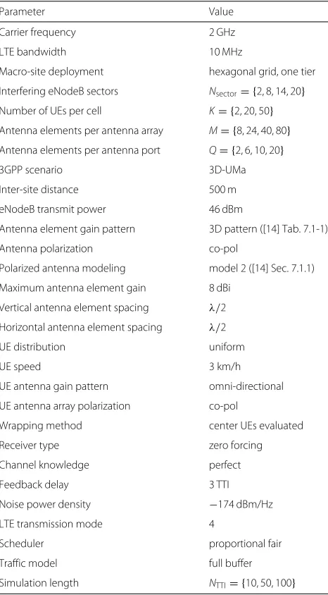
Table 2Simulation setup

Parameter Value

Carrier frequency 2 GHz

LTE bandwidth 10 MHz

Macro-site deployment hexagonal grid, one tier

Interfering eNodeB sectors Nsector= {2, 8, 14, 20}

Number of UEs per cell K= {2, 20, 50}

Antenna elements per antenna array M= {8, 24, 40, 80}

Antenna elements per antenna port Q= {2, 6, 10, 20}

3GPP scenario 3D-UMa

Inter-site distance 500 m

eNodeB transmit power 46 dBm

Antenna element gain pattern 3D pattern ([14] Tab. 7.1-1)

Antenna polarization co-pol

Polarized antenna modeling model 2 ([14] Sec. 7.1.1)

Maximum antenna element gain 8 dBi

Vertical antenna element spacing _λ/2

Horizontal antenna element spacing λ/2

UE distribution uniform

UE speed 3 km/h

UE antenna gain pattern omni-directional

UE antenna array polarization co-pol

Wrapping method center UEs evaluated

Receiver type zero forcing

Channel knowledge perfect

Feedback delay 3 TTI

Noise power density −174 dBm/Hz

LTE transmission mode 4

Scheduler proportional fair

Traffic model full buffer

Simulation length NTTI= {10, 50, 100}

that two out of the 20 interfering eNodeB sectors were taken into account but might not necessarily be the two strongest ones. Note that the strength of the interferers is of no relevance for our evaluation as we are mainly interested in simulation run times, i.e., the complexity of generating the interfering channels by means of the 3GPP 3D channel model. AssumingK = {2, 20, 50}UEs per cell at a simulation length of 20 TTI, we consider

Nsector = {2, 8, 14, 20} interfering eNodeB sectors and

M= {8, 24, 40}antenna elements per antenna array. The simulation results are provided in Fig. 9b. It is found that the run time scales linearly with the number of interfering eNodeB sectors. On the other hand, for a large number of interfering eNodeB sectors, there is a non-linearity with the number of UEs. This results from the fact that we neglect the contribution of those interferes that have a

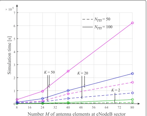
received power below a certain threshold (e.g., the noise power). Hence, the UEs will in general experience a differ-ent amount of interfering eNodeB sectors. Furthermore, we investigate simulation run times over the number M

of antenna elements assuming two simulation lengths

NTTI= {50, 100}and including all the interfering eNodeB

sectors. The simulation results are provided in Fig. 10. Again, the results exhibit an approximately linear growth in the simulation run time overMantenna elements for various numberKof UEs and various simulation lengths. Hence, in scenarios with large antenna arrays, the simu-lation run time will scale roughly proportional with the number of antenna elements.

In the next step, we compare two types of spatial chan-nel models, the 3GPP 3D model and the WINNER model. In these two models, the generation of the channel coef-ficients follows a similar procedure. The main difference is that the WINNER model is a 2D model, i.e., it does not incorporate the elevation dimension. Consequently, it only allows to apply linear antenna arrays with Q = 1. In contrast, the 3GPP 3D model enables to scrutinize 2D antenna arrays. We carry out simulations with an antenna port configuration ofNTx×NRx=4×2. In order to unveil

the impact of including the elevation information onto the simulation run time, we consider Q = {1, 2, 10}antenna elements in vertical dimension, while we are restricted to Q = 1 in the WINNER model. We evaluate various sim-ulations lengthsNTTI = {10, 50, 100}and considerK =

{2, 20, 50}UEs per eNodeB sector. The results in terms of simulation run times are provided in Fig. 11. When com-paring the simulation run times of the 3GPP 3D channel model and the WINNER model using a linear antenna array, it is observed that forK =50 UEs andNTTI=100,

the run time increases by a factor of 3.1. Thus, by tak-ing into account the elevation dimension, the simulation run time more than triples. For planar antenna arrays with Q = 10, the run time is increased by a factor of 27.49, when comparing with the WINNER model. Hence, the complexity grows roughly proportional with the number of antenna elements, which will become a prominent fac-tor for simulations of future scenarios with large antenna arrays.

3.3 Throughput performance evaluation

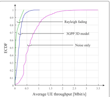
In this section, the impact of modeling both the desired as well as the interfering channels with the 3GPP 3D channel model is scrutinized. We consider a network with seven macro-sites, each employing three eNodeB sectors, and simulate 50 randomly distributed UEs per eNodeB sector. The simulation parameters are summarized in Table 2.

3.3.1 Rayleigh versus 3GPP 3D model

Fig. 9Simulation run times for various antenna array geometries, simulation lengthsNTTI, numberKof UEs, and numberNsectorof interfering

eNodeB sectors.aFixed number of interfering eNodeB sectors (one tier).bVarying number of interfering eNodeB sectors forNTTI=20

network as a baseline, (2) interference channel coefficients modeled by Rayleigh fading as used in [17], and, (3) inter-ference channel coefficients generated by the 3GPP 3D channel model. We consider four antenna ports at the transmitter, i.e.,NTx =4 and a planar antenna array with

Q = 10 linearly polarized antenna elements per antenna port. The antenna elements Q of an individual port are stacked in vertical direction with a spacing of 0.5λ, as indicated in Fig. 12. This configuration is known as

sub-array partition model since the same weight vector

Fig. 10Simulation run time [ s] over number of antenna elementsM. Dashed linesdenote a simulation length ofNTTI=50 TTI, solid lines

refer to a simulation length ofNTTI=100 TTI

ωqis applied for each port ([28] Sec. 5.2.2). The UEs are equipped with a linear antenna array consisting of two antenna elements, each being associated to an individ-ual antenna port. Figure 13 depicts the results in terms of average UE throughput statistics. It is observed that interference channel coefficients modeled by the 3GPP 3D model provide a more optimistic view on the performance

Fig. 11Simulation run times [ s] of two channel models: 3GPP 3D model and WINNER model for various simulation lengthsNTTIand

Fig. 12Antenna array port virtualization applied on system-level for co-polandcross-polpolarization modes. The antenna ports are denoted aspiwithi∈ {1,. . ., 4}. The parametersωq,q∈ {1,. . .,Q} are the phase shifts for static beamforming (e.g., electrical downtilting)

compared to Rayleigh fading, as applied in [17]. The noise-limited scenario serves as a best-case reference. A major difference between channels modeled by the 3GPP 3D model and Rayleigh fading stems from the fact that in the 3GPP 3D model, the antenna element field patterns are already incorporated in the channel coefficients, while in the Rayleigh fading case, they only affect the path loss. Consequently, the 3GPP 3D channel model has a stronger tendency to result in quasi-orthogonal signal spaces of desired and interfering signals. A systematic proof of this statement goes beyond the scope of this paper and is left for further work. Practically, our results indicate that sim-ple channel models may underestimate the throughput performance.

Fig. 13Average UE throughput [Mbit/s] ECDF curves considering three different channel models for interfering links

3.3.2 2D- versus 3D channel modeling

We evaluate system level performance in terms of aver-age UE throughput and averaver-age UE spectral efficiency applying the 3GPP 3D channel model and the WIN-NER channel model. The MATLAB implementation of the WINNER channel model is provided in [29]. For the simulation of both models, we consider the same net-work layout as shown in Fig. 3 and simulation parameters as given in Table 2. Our network comprises 50 UEs per cell and an antenna port configuration ofNTx×NRx =

4×2. For a fair comparison, we employ a UMa scenario. In the WINNER model, this corresponds to scenario C2 and is equivalent to 3GPP 3D-UMa scenario. The WIN-NER model only allows to apply linear antenna arrays with

Q = 1, whereas for the 3GPP 3D channel model, we consider a linear antenna array with Q = 1 as well as a planar antenna array with Q = 10 antenna elements in vertical direction. In the planar antenna array case, we scrutinize two electrical downtilt settingsθetilt= {0◦, 10◦}.

In the 3GPP 3D-UMa scenario, both desired and interfer-ing channels are modeled by the 3GPP 3D model, whereas in the WINNER C2 scenario, all channels are abstracted by the WINNER model. Figure 14 depicts the simulation results in terms of average UE throughput. It is observed that there is a distinct gap between the 3GPP 3D model and the WINNER model. This mainly stems from the fact that the UMa scenarios of the two models employ slightly different parameter values, e.g., for cross-correlation of the large scale parameters and the mean and standard deviation of delay- and angular spreads. When increas-ing the size of the antenna array toQ=10, the elevation dimension considered in the 3GPP 3D model remarkably

results in similar throughput values. The results indi-cate that antenna arrays withQ = 10 antenna elements per column may not achieve such effective confinement of energy as largely envisioned. Moreover, the interfer-ence suppression is highly sensitive to small errors in the weights applied to each of the antenna elements [30]. These statements have to be substantiated by system-atic investigations, yielding an interesting topic for further work. Moreover, in the 3D-UMa scenario, it is observed that when increasing the electrical downtilt angle from θetilt = 0◦toθetilt = 10◦, a slight performance

improve-ment is achieved. The effect of electrical downtilting is paled by the varying UE heights in this scenario. Figure 15 depicts the simulation results in terms of average UE spec-tral efficiency [bit/s/Hz] statistics. It is observed that for the 3GPP 3D channel model bothQ=1 andQ=10 show a similar performance for high spectral efficiency values. Similar to the throughput case, tilting slightly impacts the performance.

4 New opportunities and challenges

The integration of the 3D channel model into existing link- and system-level simulation tools paves the way for more advanced studies on the performance of a mobile cellular system in realistic environments. Existing channel models only support linear antenna arrays in the azimuth. With the introduction of the third dimension, not only higher-order MIMO schemes, but also a higher number of antenna elements per antenna array can be investi-gated. Currently, the 3GPP LTE-A standard supports up to eight antenna ports. However, recent trends aim at 100 and more antenna ports per eNodeB sector [31]. A main

Fig. 15Average UE spectral efficiency [bit/s/Hz] ECDF curves for WINNER and 3GPP 3D channel models.Solidanddashed linesshow the performance as achieved by setting the electrical tilting at 10◦ and 0◦, respectively. For the 3GPP 3D model a linear and a planar array denoted byQ=1 andQ=10 are considered

enabler for this so called massive MIMO approach will be the adoption of higher carrier frequencies, also termed

millimeter-wave communication, as it enables to consid-erably decrease the size of the antenna arrays. On the one hand, this may lead to higher complexity of the hard-ware, larger energy consumption and a greater demand for signal processing capabilities. On the other hand, it will enable a much more accurate bundling of energy towards the intended receiver, which is a key prerequisite for aggressive frequency reuse. In dense urban environ-ments, where UEs move in three dimension (consider, e.g., shopping malls, skyscrapers, and more), it is conceivable that the spectral efficiency per unit sphere might replace the area spectral efficiency as a figure of merit. Other important use cases are scenarios with high user mobility, as the number of commuters is expected to increase sub-stantially. People have become used to services following them wherever they travel. Mobile cellular access has even become a key argument to choose the means of trans-portation. Sharp, steerable beams might be an expedient solution to this issue, as they could follow a vehicle along its path.

Improvements targeting planar antenna arrays are to be further investigated. New virtualization models of antenna arrays, considering a full-connection between antenna elements, weighted in both horizontal-and verti-cal directions will lead to a better understanding of the 3D beamforming. Moreover, new two-dimensional codebook designs are necessary for the evaluation of FD-MIMO.

5 Conclusions

Remarkably, taking into account a planar antenna array results in performance degradation. This result indicates, that the beams might not be as sharp as largely envi-sioned. A systematic evaluation of this behavior is left for further work. The paper is completed by an elaboration on new opportunities that became possible with the 3D channel model, and the challenges ahead to realize the full potential of the upcoming new technologies. Our imple-mentation approach is openly accessible, and our hope is to inspire researches and developers of link- and sys-tem level simulation tools to further elaborate and develop these topics by applying it.

Competing interests

The authors declare that they have no competing interests.

Acknowledgments

This work has been funded by A1 Telekom Austria AG, and the KATHREIN-Werke KG. The financial support by the Federal Ministry of Economy, Family and Youth and the National Foundation for Research, Technology and Development is gratefully acknowledged.

Received: 14 August 2015 Accepted: 4 February 2016

References

1. S Ahmadi,LTE-Advanced: a practical systems approach to understanding 3GPP LTE releases 10 and 11 radio access technologies. (ITPro collection, Elsevier Science, 2013)

2. J Ikuno, M Wrulich, M Rupp, inVehicular Technology Conference (VTC 2010-Spring). System level simulation of LTE networks, (2010), pp. 1–5. doi:10.1109/VETECS.2010.5494007

3. A Rodriguez-Herrera, S Mcbeath, D Pinckley, D Reed, inIEEE 62nd Vehicular Technology Conference, VTC-2005-Fall. Link-to-system mapping

techniques using a spatial channel model, vol. 3, (2005), pp. 1868–1871. doi:10.1109/VETECF.2005.1558430

4. P Matthias,Mobile fading channels. (John Wiley and Sons, Inc., New York, NY, USA, 2002)

5. J Parsons,The mobile radio propagation channel, 2nd edn. (John Wiley and Sons, Inc., New York, NY, USA, 2000)

6. P Almers, E Bonek, A Burr, N Czink, M Debbah, V Degli-Esposti, H Hofstetter, P Kyosti, D Laurenson, G Matz, A Molisch, C Oesteges, H Ozcelik, Survey of channel and radio propagation models for wireless MIMO systems. EURASIP J. Wireless Commun. Networks (2007). doi:10.1155/2007/19070 7. A Paulraj, R Nabar, D Gore,Introduction to space-time wireless

communications. (Cambridge University Press, 2003)

8. 3GPP TR36.996,Spatial channel model for multiple input multiple output (MIMO) simulations. (3rd Generation Partnership Project (3GPP), 2003) 9. WINNER I WP5, Final report on link level and system level channel models.

IST-2003-507581 WINNER I Deliverable D5.4 (2005). http://www.ist-winner.org/phase_model.html

10. WINNER II WP1, WINNER II channel models. IST-4-027756 WINNER II Deliverable D1.1.2 (2007). http://www.ist-winner.org/phase_2_model. html

11. ITU-R and M.2135, Guidelines for evaluation of radio interface technologies for IMT-Advanced. Report (2009). https://www.itu.int/ dms_pub/itu-r/opb/rep/R-REP-M.2135-1-2009-PDF-E.pdf 12. E Larsson, O Edfors, F Tufvesson, T Marzetta, Massive MIMO for next

generation wireless systems. IEEE Commun. Mag.52(2), 186–195 (2014). doi:10.1109/MCOM.2014.6736761

13. Y Song, X Yun, S Nagata, L Chen, inIEEE International Conference on Communications Workshops (ICC). Investigation on elevation beamforming for future LTE-Advanced, (2013), pp. 106–110. doi:10.1109/ICCW.2013.6649210

14. 3GPP TR36.873,Study on 3D channel model for LTE, v12.2.0. (3rd Generation Partnership Project (3GPP), 2014)

15. A Kammoun, H Khanfir, Z Altman, M Debbah, M Kamoun, Preliminary results on 3D channel modeling: From theory to standardization. IEEE J. Selected Areas Commun.32(6), 1219–1229 (2014).

doi:10.1109/JSAC.2014.2328152

16. Z Hu, R Liu, S Kang, X Su, J Xu, inInternational Conference on

Communications and Networking in China (CHINACOM). Work in progress: 3D beamforming methods with user-specific elevation beamfoming, (2014), pp. 383–386. doi:10.1109/CHINACOM.2014.7054323 17. F Ademaj, M Taranetz, M Rupp, Implementation, Validation and

Application of the 3GPP 3D MIMO Channel Model in Open Source Simulation Tools. Paper presented at the Twelfth International Symposium on Wireless Communication Systems, ISWCS, 25-28 August 2015

18. Vienna LTE-A Simulators. http://www.nt.tuwien.ac.at/research/mobile-communications/vienna-lte-a-simulators/. Accessed 14 Aug 2015 19. H Masui, T Kobayashi, M Akaike, Microwave path-loss modeling in urban

line-of-sight environments. IEEE J. Selected Areas Commun.20(6), 1151–1155 (2002). doi:10.1109/JSAC.2002.801215

20. A Weber, A Bestard, in8th International Symposium on Wireless

Communication Systems (ISWCS), 2011. Modeling of X-pol antennas for LTE system simulation, (2011), pp. 221–225. doi:10.1109/ISWCS.2011.6125342 21. S Schwarz, J Ikuno, M Simko, M Taranetz, Q Wang, M Rupp, Pushing the

limits of LTE: A survey on research enhancing the standard. IEEE Access.1, 51–62 (2013). doi:10.1109/ACCESS.2013.2260371

22. M Taranetz, T Blazek, T Kropfreiter, MK Müller, S Schwarz, M Rupp, Runtime precoding: enabling multipoint transmission in LTE-Advanced system-level simulations. IEEE Access.3, 725–736 (2015).

doi:10.1109/ACCESS.2015.2437903

23. 3GPP TS 36.201,LTE Physical Layer - General Description, v9.0.0. (3rd Generation Partnership Project (3GPP), 2009)

24. Y Wang, J Xu, L Jiang, Challenges of system-level simulations and performance evaluation for 5G wireless networks. IEEE Access.2, 1553–1561 (2014). doi:10.1109/ACCESS.2014.2383833

25. 3GPP 325.996,Spatial channel model for Multiple Input Multiple Output (MIMO) simulations, v12.0.0. (3rd Generation Partnership Project (3GPP), 2012)

26. 3GPP TSG RAN WG-1 R1-140048,Phase 2 calibration results for 3D channel model. Meeting report, (2014)

27. 3GPP TSG RAN WG-1 R1-143469,Summary of 3D-channel model calibration results. Meeting report, (2014)

28. 3GPP TR36.897,Elevation Beamforming/Full-Dimension MIMO for LTE, v0.3.1. (3rd Generation Partnership Project (3GPP), 2015)

29. L Hentila, P Kyosti, M Kaske, M Narandzic, M Alatossava, Matlab implementation of the winner phase II channel model ver1.1 (2007). http://projects.celtic-initiative.org/winner+/phase_2_model.html. Accessed Sep. 2008

30. O Bakr, M Johnson, R Mudumbai, U Madhow, in47th Annual Allerton Conference on Communication, Control, and Computing Allerton. Interference suppression in the presence of quantization errors, (2009), pp. 1161–1168

31. F Rusek, D Persson, BK Lau, E Larsson, T Marzetta, O Edfors, F Tufvesson, Scaling up MIMO: Opportunities and challenges with very large arrays. IEEE Signal Process. Mag.30(1), 40–60 (2013).