R E S E A R C H
Open Access
Low complexity and high accuracy angle of
arrival estimation using eigenvalue
decomposition with extension to 2D AOA and
power estimation
Saleh O Al-Jazzar
1*, Artem Muchkaev
2, Ahmad Al-Nimrat
3and Mahmoud Smadi
3Abstract
In this paper, an angle of arrival (AOA) estimator is presented. Accurate AOA estimation is very crucial for many applications such as wireless positioning and signal enhancement using space processing techniques. The proposed estimator is based upon applying the eigenvalue decomposition (EVD) method on the crosscorrelation matrix of the received signals at two sides of the antenna array doublets. The proposed method is named the eigenvalue-decomposition-based AOA (EDBA) estimator. In comparison with the ESPRIT algorithm, the EDBA has less complexity because the decomposition in the EDBA method is performed only once and on a smaller matrix dimension than that in the ESPRIT algorithm where the decomposition is performed twice. The other advantage is that the EDBA method has better performance than the ESPRIT algorithm. The EDBA is also extended to two-dimensional (2D) AOA estimation with automatic pairing in two ways. The first one performs the 2D AOA estimation by considering the eigenvalues of the crosscorrelation matrix to estimate the azimuth angles and their corresponding eigenvectors to estimate their corresponding elevation angles. Thus, the 2D AOA estimation is performed with automatic pairing and without the need for any pairing or searching techniques. The first 2D extension of the EDBA is named the EDBA-2D estimator. Another 2D AOA estimator that is based upon the EDBA method is also presented and named the Two-EDBA estimator. This second 2D estimator performs the pairing between the azimuth and elevation angles using the alignment of the eigenvalues’magnitudes. An additional advantage for the EDBA estimator is the fact that it provides an estimate for the received signal power paired automatically with its corresponding AOA estimate. Simulations of the proposed EDBA method and its 2D extensions with the signals’power estimation are shown to assess their performance.
1 Introduction
Many applications require accurate estimation of the angle of arrival (AOA) of the received signal. Examples of these applications are signal reception enhancement [1,2] and accurate wireless positioning [3,4]. Many effects cause errors in the AOA estimation. An error in the AOA estimate can cause huge error when locating wireless devices or an increase in the bit error rate when detecting the received signal. Thus, it is of interest to develop techniques to estimate the AOA accurately.
In some cases, it is required to estimate two-dimen-sional (2D) angles, i.e., the azimuth and elevation angles. Besides the accuracy requirement for estimating both the azimuth and elevation angles, it is of interest to pair them for each of their corresponding source. The com-plexity of the estimator is another issue that requires the designers of the estimator to take care of. Also, in 2D AOA estimation, the antenna array geometry plays an important role in the estimation procedure. In this paper, we will assume two antenna array geometries and we will provide a 2D estimator, based upon the pro-posed estimator, for each of these geometries. The first one is the rectangular antenna array shape formulated from two-parallel uniform linear arrays (ULAs). The * Correspondence: [email protected]
1Electrical Engineering Department, University of Ha’il, Ha’il, Saudi Arabia
Full list of author information is available at the end of the article
second antenna array geometry considered in this paper is theL-shaped antenna array formulated from two per-pendicular ULAs.
ESPRIT or ESPRIT-based algorithms are proposed in the literature to perform the 2D AOA estimation, such as in [5-8]. Also, another method proposed to perform the pairing procedure is the modified propagator method (PM) [9,10]. Although these methods do not require complex searching techniques as in [11-14], they still require pairing techniques in matching the angles estimated. The 2D AOA estimator proposed in [15] uses two-parallel ULAs, whereas the method in [16] is based upon matrix enhancement and the matrix pencil algo-rithm. The proposed method in [17] constructs a sec-ond-order statistic based upon the Schur-Hadamard product steering vector to perform the 2D AOA estima-tion. In [18], the authors propose an estimator that requires two ULAs to pair the azimuth and elevation angles. In [19-22], the authors propose 2D AOA techni-ques that apply singular value decomposition (SVD) on specially constructed covariance matrices.
In this paper, we propose an AOA estimator that enhances the AOA estimation with low computational complexity. The proposed AOA estimator utilizes the eigenvalue decomposition (EVD) method and is named the eigenvalue decomposition-based AOA (EDBA) esti-mator. The EDBA applies the EVD on a crosscorrelation matrix constructed from both sides of the antenna array doublets.
The first advantage of the proposed EDBA method is its low complexity. In fact, it has lower computational complexity than that of the well-known ESPRIT algo-rithm due to the fact that the decomposition used in the EDBA method is applied only once and on a smaller matrix dimension than that in the ESPRIT algorithm where the decomposition is applied twice [23]. The sec-ond advantage of the proposed methods is its better performance in estimating the AOA than that of the ESPRIT algorithm. Another benefit for using the EDBA method is its ability to estimate the received signals’ power with automatic pairing with their corresponding AOA estimates.
The EDBA is also extended for 2D AOA estimation in two ways. The first one is named the EDBA-2D method. In this extension, the azimuth and elevation angles are estimated and paired automatically. The EDBA-2D method starts by formulating a crosscorrelation matrix from the received signals at both sides of two-parallel ULAs. Then, the azimuth angles are estimated from the eigenvalues of the crosscorrelation matrix, and the ele-vation angles are estimated from the corresponding eigenvectors of the same crosscorrelation matrix. Thus, automatic pairing between the estimated azimuth and elevation angles is provided by the correspondence
between the eigenvalues and the eigenvectors of the crosscorrelation matrix. The second way presented to extend the EDBA method for 2D AOA estimation uses the EDBA method twice and separately at the two ULAs of the L-shaped antenna array to estimate the azimuth and elevation angles. Then, we pair them with their cor-responding sources using the alignment of the eigenva-lues’magnitudes. This method is named the Two-EDBA estimator. The EDBA-2D and Two-EDBA methods have the advantage of not requiring any searching process as well as possessing the advantages of the EDBA method over the ESPRIT algorithm as discussed above.
The paper is organized as follows: Section 2 intro-duces the system model that forms the foundation for the EDBA estimator. The proposed EDBA estimator is explained in Section 3. Section 4 presents the 2D AOA system models. The proposed 2D extensions for the EDBA method are presented in Section 5. Estimating the received signals’ power is presented in Section 6. The simulated performance of the EDBA estimator and its 2D extensions with the signals’power estimation are presented in Section 7. Finally, conclusions are shown in Section 8.
2 System model for the EDBA estimator
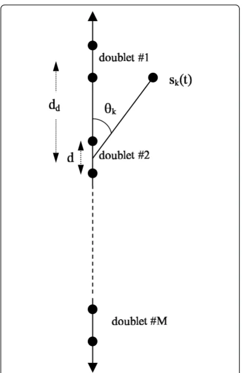
In this section, we present the narrowband received sig-nal model that will be utilized for the AOA estimation. The antenna array is formed fromM uniform antenna doublets (i.e., 2M total antenna elements) as shown in Figure 1. Each antenna doublet is formed of two antenna elements spaced by a distanced. We assume a
KBPSK sources signals,{ˇsk(t)}Kk=1, impinging upon the antenna array. The signal ˇsk(t) is represented as
ˇ
sk(t) =sk(t) cos(2πfct) ={sk(t) exp(j2πfct)}where fc is the carrier frequency and sk(t) =
iαk(i)g(t−iT), i is an integer which represents the time index andsk(t) is the complex low-pass equivalent of ˇsk(t),T is the sym-bol period, ak(i) = Akbk(i) wherebk(i)Î (-1, + 1) which represents the symbol parity and Ak is a positive con-stant which represents the amplitude ofsk(t) andg(t) is the (raised cosine) pulse shaping function with
g(nT) =
r1(i) = K
k=1
αk(i)a(θk) +n1(i) (2)
where
a(θk) =
a1(θk)· · ·aM(θk) T
(3)
and
am(θk) = exp
j2π
λ dd×(m−1) cos(θk)
(4)
with l is the signal wavelength, dd is the distance between consecutive antenna doublets, and θk is the AOA for thekth signal. In addition, n1(i) is the noise vector added to the received signal at the antenna ele-ments located at the upper part of the antenna doublets, which is additive white Gaussian noise (AWGN) and has a covariance matrix of s2 IM ×M, where IM ×Mis theM ×M identity matrix. Finally, (.)T represents the transpose operation.
The (M× 1) received signal vector can be written in a matrix form as
r1(i) =A(θ)α(i) +n1(i)
where
A(θ) = [a(θ1)· · ·a(θK) ] (5) and
α(i) =α1· · ·αK T
with
θ =θ1· · ·θK T
.
From now on, we will drop the term (i) from all terms for simplicity.
The received signal vector at the lower part of the antenna doublets set, shown in Figure 1, will be given the notationr2. Thus,
r2=A(θ)Zα+n2
where
Z= diag[z1· · · zk· · · zK] (6) with
zk= exp
j2π
λ d×cos(θk)
(7)
andn2 is an AWGN at the lower side of the antenna array doublets.
Now we showed the received signal model at the antenna arrays, and we will next propose the EDBA estimator.
3 Proposed eigenvalue-decomposition-based AOA (EDBA) estimator
To implement the EDBA method, we start by formulat-ing a crosscorrelation matrix (R21) betweenr2andr1 as follows
R21=E[r2rH1] =A(θ)PsZA(θ)H (8)
where
Ps:=E[ααH] = diag ( [p1· · ·pk· · ·pK] ) (9) wherepkis the power of thekth received signal. We use here the assumption that n1 andn2are inde-pendent realizations of AWGN.
Considering the eigenvalue decomposition ofR21 as follows
R21=UZUH (10) whereΓZis a diagonal matrix with its diagonal con-taining the eigenvalues ofR21, i.e.,
Z= diag ( [γ1· · ·γm· · ·γM] )
where the largestKvalues of the diagonal elements of ΓZcorrespond to the Ksources which we will callg1®K ≡g1 ®gK. Each element ofg1®Kcorresponds to one of theKsources.
Now, from the EVD of R21 shown in (10), and from the definition ofR21in (8), we have
A(θ)PsZA(θ)H=UZUH (11)
and so we can say
A(θ) =UT (12)
whereTis the appropriate matrix to change the basis vectors.
By substituting (12) into (11), we can write
Z=TPsZTH. (13)
The matrixΓZis anM ×Mmatrix, andZandPsare
K×Kdiagonal matrices. Also, the nonzero diagonal ele-ments of ΓZ are only the firstKdiagonal elements and then (13) can be written as
⎡
Looking at (14), we can deduce that the matrix T should beM×K. Also, the lower (M -K) ×Kpart ofT should be all zero elements, i.e.,
T=
But, the left-hand side of (18) is a diagonal matrix, and the matrices Psand Z are diagonal as well. So, from (18), we can deduce that the matrixϒ is diagonal too, i. e.,
Now, the eigenvector matrixUis defined as
U=u1· · · uk· · · uK· · · uM
(20)
whereuk is the kth column eigenvector ofR21, and the K columns of U that correspond to the Klargest (which are also nonzero) eigenvalues of R21 will be given the notation U¯, i.e., plied by the zero matrix in (17), then the eigenvector matrix (U)¯ and the matrixA(θ) span the same signal subspace, and we have
A(θ) =U¯ϒ (22)
or
¯
U=A(θ) (23)
whereΩ=ϒ-1and is a diagonal matrix (since ϒis a diagonal matrix). Thus, each column of U¯ is a rotated scaled version of a corresponding column inA(θ).
col-where
ζk=
M−1
μ=1
aμ+1(θk)
aμ(θk)
M−1 .
(25)
AlthoughA(θ) (from whicha(θk) and consequentlyaμ (θk) can be deduced) is not available at the receiver, still we could deduce the matrix U¯ fromU. Thus, looking back at (25) in whichζkis expressed in terms the ele-ments of a(θk), and becauseuk is a rotated scaled ver-sion ofa(θk), thenζkthat is the average relative phase between two consecutive elements of a(θk) can be expressed in terms of two corresponding consecutive elements ofukas follows
ζk=
M−1
μ=1 uk,μ+1
uk,μ
M−1
(26)
whereuk,μis theμth element of the vectoruk. Thus,θkcan be estimated as follows
ˆ
θk= cos−1 λζ
k 2πdd
. (27)
The performance of the proposed method will be shown in the simulation section (Section 7). In compari-son with the ESPRIT method, the EDBA uses the EVD on an M ×M matrix as shown in (10), whereas in the ESPRIT method, the EVD will be applied on a 2M × 2Mfor the same system model assumed [23]. Also, the EVD in the EDBA is applied only once, whereas in the
ESPRIT method, the EVD is applied twice for estimating the AOA as shown in [23]. Next, we will present the system models that will be used for the extension of the EDBA method for estimating the 2D AOA with auto-matic pairing.
4 System model for 2D AOA estimation
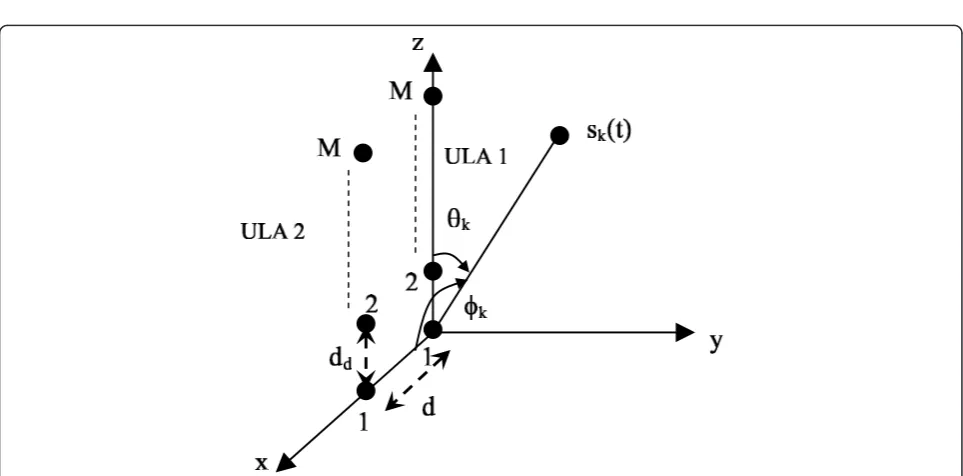
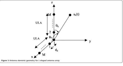
For the 2D estimation, we will present two ways to extend the EDBA method to estimate the azimuth and elevation angles. There are two antenna alignments over which the extension will be presented. In the first antenna alignment, we will assume the parallel ULAs shown in Figure 2. The second antenna alignment that we will consider is the L-shaped antenna array illu-strated in Figure 3. In the next subsections, we will pro-vide more insight into the system models for the parallel ULA and theL-shaped antenna array.
4.1 Parallel ULA
The parallel ULA is formed from M antenna parallel doublets (i.e., 2M total antenna elements) as shown in Figure 2. Each antenna doublet is formed of two antenna elements spaced by a distanced. To start devel-oping the received signal model, first consider the sampled received signal after the matched filter stage (rA) at the antenna elements that are located on the right-hand side of each antenna doublets, shown in Fig-ure 2, which is represented as
rA= K
k=1
αka(˜ θk) +nA (28)
where
˜
a(θk) =
˜
a1(θk)· · · ˜aM(θk)
T (29)
and
˜
am(θk) = exp
j2π
λ dd×(m−1) cos(θk)
(30)
withlis the signal wavelength andddis the distance between consecutive antenna elements at each ULA. In addition,nAis the noise vector added to the received sig-nal at the antenna elements (fromm= 1®M) located along the right-hand side of each antenna doublet, which is AWGN and has a covariance matrix ofs2IM×M.
The (M × 1) received signal vector can be written in matrix form as
rA=A(˜ θ)α+nA where
˜
A(θ) = [a(˜ θ1)· · · ˜a(θK) ]. (31) The received signal vector at the left-hand side of the antenna doublets set, shown in Figure 2, will be given the notationrB. Thus,
rB=A(˜ θ)Yα+nB where
Y= diagy1. . .yk· · · yK
(32)
with
yk= exp
j2π
λ d×cos(φk)
(33)
and nB is an AWGN vector at the left-hand side of the antenna array doublets.
The next subsection will provide some insight into the
L-shaped antenna array.
4.2 TheL-shaped antenna array
The L-shaped antenna array is formed of two perpendi-cular antenna arrays as shown in Figure 3. The sampled received signal (rz) at the antenna elements (after the matched filter stage) that are located in thez-axis direc-tion is represented as
rz= K
k=1
αka(θk) +nz (34)
wherenzis the AWGN noise vector with a covariance matrix ofs2IM×M.
Similarly, the sampled received signal at the antenna elements, fromm= 1 tom=M, that are located in the
x-axis direction is given the notationrx and is repre-sented as
rx= K
k=1
αkb(φk) +nx (35)
whereb(jk) = [b1(jk) ...bM(jk)]Tand
Likewise, nx is the AWGN noise vector, and it also has a covariance matrix ofs2IM×M.
So both (M× 1) received signal vectors can be written in matrix form as
rz=A(θ)α+nz
and
rx=B(φ)α+nx
where
B(φ) = [b(φ1)· · · b(φK) ]. (36) Thus, the received signal models for the different 2D antenna arrays structures are presented.
5 Extension of the EDBA for 2D AOA estimation
In this section, we will propose two methods for which the EDBA can be used to estimate the azimuth and ele-vation angles with automatic pairing. The first method is named the EDBA-2D method that is based upon the parallel antenna array structure illustrated in Figure 2. The second method is named the Two-EDBA method that is based upon the L-shaped antenna structure in Figure 3.
5.1 Proposed EDBA-2D estimator
The EDBA-2D method is based upon the system model introduced in Section 4.1 and illustrated in Figure 2. The EDBA-2D estimation starts by formulating a cross-correlation matrix (RBA) betweenrBandrAas follows
RBA =E[rBrA] =A(˜ θ)PsYA(˜ θ)H. (37) Considering the eigenvalue decomposition ofRBAas follows
RBA=U˜˜YU˜ H
(38)
where ˜Y is a diagonal matrix with its diagonal con-taining the eigenvalues ofRBA, i.e.,
˜
Y= diag([γ˜1· · · ˜γm· · · ˜γM] )
where the largestKvalues of the diagonal elements of
˜
correspond to the K sources which we will call
˜
γ1→K≡ ˜γ1→ ˜γK. Each element of γ˜1→K corresponds to one of the K sources. Also, U¯ is the eigenvector matrix forRBA.
Now, from the EVD ofRBAshown in (38), and from the definition ofRBAin (37), we see that
˜
where T˜ is the appropriate matrix to change the basis vectors.
By substituting (40) into (39), we can write
˜
Y=TP˜ sYT˜ H
. (41)
The matrix ˜Y is anM×M matrix andPs andY are
K×Kdiagonal matrices. Also, the nonzero diagonal ele-ments of ˜ are only the first K diagonal elements. Thus, (41) can be written as
⎡
Looking at (42), we can deduce that the matrix ˜ should be M ×K. Also, the lower (M - K) ×K part of
˜
should be all zero elements, i.e.,
˜
(45), we can deduce that the matrix T˜ is diagonal too, i.
Substituting (46) in (42) and looking at the nonzero diagonal elements in both sides of (42), i.e., γ˜1→ ˜γK, the following equation can be deuced:
˜
γk=˜tk,kt˜k∗,kpkyk
where (.)* is the complex conjugate operator. Thus,
˜
γk= |˜tk,k|2pkyk. (47)
Since |˜tk,k|2 is a magnitude square andpk is a power variable, then both terms are not complex variables. Thus, looking at both sides of (47), then
γ˜k= yk. (48)
But the azimuth angle (jk) is implicated in ∠ykas can be deuced from (33). Thus, the azimuth angle can be estimated from the eigenvalue ofRBAas follows
ˆ
For the elevation angle (θk), it is estimated from the eigenvectors ofRBAin a similar way as discussed in the EDBA estimator explained in Section 3. We will not repeat the discussion and derivation again in this section but rather we will give the final procedure on how to estimate the elevation angleθk.
We can calculate ζ˜k which is the average relative phase between two consecutive elements of a(˜ θk) in terms of two corresponding consecutive elements of u˜k as follows Thus,θkcan be obtained as follows
ˆ
Because of eigenvalue-eigenvector correspondence, estimation of the azimuth angle (jk) for the kth signal from the kth eigenvalue (γ˜k) and its corresponding
elevation angle (θk) from the corresponding kth eigen-vector (u˜k) is performed with automatic pairing and without the need of any pairing procedure.
5.2 Proposed two-EDBA estimator
The Two-EDBA method is based upon the L-shaped antenna structure in Figure 3. The Two-EDBA starts by estimating the azimuth and elevation angles separately. This is a straightforward procedure using the EDBA method on each of the received signals on both ULAs at each axis. Then, after estimating the azimuth (jk) and elevation (θk) angles, the pairing is achieved by the alignment of the eigenvalues’magnitudes. From Section 3, it is shown that the EDBA method estimates the angles from the eigenvectors of the crosscorrelation matrix R21. Since the eigenvalues’ magnitudes of the crosscorrelation matrixR21 depend on the received sig-nals’power (which are assumed to be the same on both ULAs on both axis), then the pairing between the esti-mated azimuth and elevation angles is achieved by align-ing the estimated azimuth and elevation angles depending on their corresponding eigenvalues’ magnitudes.
6 Estimating the received signals’power
This section shows how the received signals’power can be estimated after estimating the received signals’ AOAs. This is achieved with an automatic pairing between the received signals’power with their corre-sponding AOAs. Pairing can be performed for the EDBA estimator or its 2D estimator extensions. For sake of simplicity, we will show how the received sig-nals’power is estimated for the simple EDBA estimator explained in Section 3, and the extension for the 2D EDBA estimators can be easily deduced.
To explain how the received signals’ power is esti-mated, let us assume first that the angles of the received signals using the EDBA method are estimated as explained in Section 3. Then, the vectora(θk) in (3) and (4) can be reformulated using the estimated angles (θˆk) for k= 1® K. This leads to the ability of reformulating the matrix A(θ) in (5), and we will give it the notation
ˆ
A(θ). Since the eigenvector matrixU is available from (10), and the matrix A(ˆ θ) is known, then the appropri-ate matrix (T) in (12) can be estimated as follows
ˆ
T=U−1A(ˆ θ).
Similarly, the matrix Zdepends onθk in its formula-tion as shown (6) and (7). Thus, from θˆk, we can refor-mulate the matrixZ, and we will give it the notation Zˆ.
(Ps) can be estimated as follows
ˆ
Ps =Tˆ +
ZTˆ +Hˆ
Z−1 (51)
where (.)+ is the pseudo-inverse operator.
Thus, the received signal power can be deduced from the diagonal elements of Pˆs, and we will give it the notation pˆk. The pairing between θˆk and pˆk is
automatically provided from the fact that θˆk is esti-mated from the eigenvectors in Uand ˆpk is estimated from their corresponding eigenvalues in ΓZ. Since each eigenvector inU corresponds automatically to a specific eigenvalue in ΓZ, then θˆk is automatically paired with its corresponding pˆk. Thus, the estimation of the received signal power is estimated with
0 5 10 15
10−2 10−1 100 101
SNR in dB
RMSE in degrees
ESPRIT W=256 EDBA W=256 ESPRIT W=1000 EDBA W=1000
Figure 4Root-mean-square error (RMSE) of angle estimation in degrees versus signal to noise ratio (SNR) in dB for (θ1,2= 75°, 45°).
0 5 10 15
10−1 100 101
SNR in dB
RMSE in degrees
ESPRIT W=256 EDBA W=256 ESPRIT W=1000 EDBA W=1000
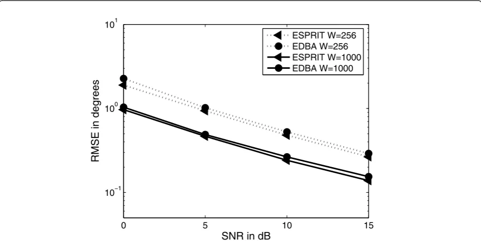
Figure 5Root-mean-square error (RMSE) of angle estimation in degrees versus signal to noise ratio (SNR) in dB for (θ1,2= 75°, 45°)
2 3 4 5 6 7 8 10−2
10−1 100 101
AOA deviation (
δ
) in degrees
RMSE in degrees
ESPRIT W=256 EDBA−2D W=256 ESPRIT W=1000 EDBA−2D W=1000
Figure 6Root-mean-square error (RMSE) of angle estimation in degrees versus angular deviation with SNR = 10 dB for (θ1,2= 75°,
45°), (j2= 55°) and (j1=j2+δ).
−10
−5
0
5
10
15
20
10
−410
−310
−210
−110
0SNR in dB
Power RMSE
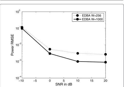
EDBA W=256
EDBA W=1000
automatic pairing with its corresponding received sig-nal AOA.
Similarly, the estimation of the received signal power can be easily applied to the 2D AOA estimation exten-sions for the EDBA explained in Section 5, resulting in estimating the azimuth/elevation angles jointly with the received signals’power with automatic pairing.
The performance of the proposed methods will be shown in the simulation section (Section 7).
7 Simulation results
Simulations of the proposed EDBA estimator with its extensions were completed to assess their performance. The elements of each antenna array were separated by a half-wavelength (i.e., d= λ2). Unless mentioned other-wise, the number of antenna doublets was set to M = 10. The number of snap shots was set to W= 256 and
W= 1,000 (where Wis the number of snap shots over which the correlation matrices were estimated). The number of sources was set to 2. The near far ratio (NFR) was set to -10 dB, where the NFR is defined as 10 log
A2
2
A2 1
). The proposed EDBA and its extensions were compared with the ESPRIT method.
Figure 4 shows the root-mean-square error (RMSE) of the angle estimation in degrees for the proposed EDBA method compared with the ESPRIT method for different signal to noise ratios (SNR)s. Since the power for both sources was not equal, then we assumed that the SNR was taken for the first source. The angles for the two sources were set toθ1 = 75° andθ2= 45°. The results in Figure 4 show that the proposed EDBA method gave better performance than the ESPRIT method.
Figure 5 shows the RMSE of the angle estimation in degrees for the proposed EDBA-2D method compared with the ESPRIT method for different SNRs. The ele-vation angles for the two sources were set toθ1 = 75° and θ2 = 45°. The azimuth angles for the two sources were set to j1 = 80° andj2 = 55°. The results in Fig-ure 5 indicate that the proposed EDBA-2D method gave very close performance to the ESPRIT method with the less complexity advantage for the proposed EDBA-2D method. Also, the EDBA-2D performs the estimation of the azimuth and elevation angles with automatic pairing.
The simulation presented in Figure 6 shows the RMSE for the proposed EDBA-2D method compared with the ESPRIT method for different source angle deviation.
Table 4 Table of successful pairing rate using the proposed EDBA-2D and Two-EDBA algorithm compared to the algorithm in [14] and the SVD-based algorithm in [22] for different number of antenna elements andW= 1, 000
M Algorithm in [14](%) SVD-based algorithm in [22](%) EDBA-2D (%) Two-EDBA (%)
6 97.1 100 100 100
10 99.7 100 100 100
Table 3 Table of successful pairing rate using the proposed EDBA-2D and Two-EDBA algorithm compared to the algorithm in [14] and the SVD-based algorithm in [22] for different number of antenna elements andW= 256
M Algorithm in [14](%) SVD-based algorithm in [22](%) EDBA-2D (%) Two-EDBA (%)
6 59.4 98.6 100 100
10 67.3 99.8 100 100
Table 2 Table of successful pairing rate using the proposed EDBA-2D and Two-EDBA algorithm compared to the algorithm in [14] and the SVD-based algorithm in [22] for different SNRs andW= 1,000
SNR (dB) Algorithm in [14](%) SVD-based algorithm in [22](%) EDBA-2D (%) Two-EDBA (%)
15 99.7 100 100 100
20 100 100 100 100
25 100 100 100 100
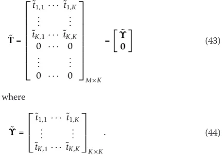
Table 1 Table of successful pairing rate using the proposed EDBA-2D and Two-EDBA algorithm compared to the algorithm in [14] and the SVD-based algorithm in [22] for different SNRs andW= 256
SNR (dB) Algorithm in [14](%) SVD-based algorithm in [22](%) EDBA-2D (%) Two-EDBA (%)
15 65.7 100 100 100
20 94.4 100 100 100
The angular deviation is performed by setting j1to be taken from the following equationj1 =j2+δwhereδ is the angular deviation with θ1 = 75°,θ2 = 45°, andj2 = 55°. The SNR for the first source was set to 10 dB. The results in Figure 6 indicate that the proposed EDBA-2D method gave better performance than the ESPRIT method for different AOA deviations.
In Figure 7, the simulation shows the power RMSE for the proposed EDBA for different SNRs. The results in Figure 7 show that the EDBA method managed to esti-mate the received signal power with high accuracy.
Tables 1 and 2 show the pairing success rate for the proposed EDBA-2D and Two-EDBA algorithms com-pared to the algorithm in [14] and the SVD-based algo-rithm in [22] for different SNRs in dB with W= 256 and W= 1, 000, respectively. The number of antenna elements Mwas set to 10. Both tables indicate that the proposed EDBA-2D and Two-EDBA algorithms mana-ged to pair the azimuth and elevation angles successfully.
Tables 3 and 4 show the pairing success rate for the proposed EDBA-2D and Two-EDBA algorithms com-pared to the algorithm in [14] and the SVD-based algo-rithm in [22] for different number of antenna elements with W= 256 and W= 1, 000, respectively. The SNR was set to 15 dB for the first source. Both tables show that the proposed EDBA-2D and Two-EDBA algorithms managed to pair the azimuth and elevation angles successfully.
Thus, the proposed EDBA-2D and Two-EDBA meth-ods have high capability of pairing the estimated azi-muth and elevation angles with good accuracy and in an automatic procedure.
8 Conclusion
In this paper, we propose an AOA estimator that we named the EDBA method. The EDBA method is applied by taking the EVD of the received signal crosscorrela-tion matrix. The AOA of the received signals is con-tained in the eigenvectors of the crosscorrelation matrix. So, the AOA of the received signals is deduced from these eigenvectors. Two extension methods for 2D mation are introduced. The first extension method esti-mates the elevation angles from the eigenvectors of the crosscorrelation matrix, and the corresponding azimuth angles are estimated from the corresponding eigenva-lues. This method is named the EDBA-2D. The second extension method is named the Two-EDBA estimator and uses the alignment of the eigenvalues’magnitudes to pair the azimuth and elevation angles. Also, the EDBA method is extended to estimate the received sig-nals’ power with automatic pairing with their corre-sponding AOAs. Numerical simulation indicated that the EDBA method and its extensions outperformed the
ESPRIT AOA estimator and other pairing methods. Also, the EDBA method and its extensions are low com-plex and do not require any searching or pairing proce-dure to perform the estimation.
Author details
1Electrical Engineering Department, University of Ha’il, Ha’il, Saudi Arabia 2
Aerospace Engineering Department, Korea Advanced Institute of Science and Technology (KAIST), Daejeon, South Korea3Electrical Engineering
department, Hashemite University, Zarqa, Jordan
Competing interests
The authors declare that they have no competing interests.
Received: 9 July 2011 Accepted: 7 October 2011 Published: 7 October 2011
References
1. N Hew, N Zein, Space-time estimation techniques for UTRA system. Capacity and range enhancement techniques for the third generation mobile communications and beyond (Ref. No. 2000/003). IEE Colloquium on, 6/1–6/7 (Feb. 2000)
2. Y-F Chen, M Zoltowski, Joint angle and delay estimation for DS-CDMA with application to reduced dimension space-time RAKE receivers. Acoustics, speech, and signal processing, 1999, inICASSP‘99. Proceedings, 1999 IEEE International Conference on.5, 2933–2936 (March 1999)
3. S Al-Jazzar, M Ghogho, D McLernon, A joint TOA/AOA constrained minimization method for locating wireless devices in non-line-of-sight environment. IEEE Trans Veh Technol.59, 468–472 (2009)
4. P Deng, P Fan, An AOA assisted TOA positioning system. Communication technology proceedings, 2000. WCC–ICCT 2000, inInternational Conference on.2, 1501–1504 (August 2000)
5. S Kikuchi, H Tsuji, A Sano, Pair-matching method for estimating 2-D angle of arrival with a cross-correlation matrix. IEEE Antennas Wirel Propag Lett.5, 35–40 (2006)
6. R Roy, T Kailath, ESPRITestimation of signal parameters via rotational invariance techniques. Opt Eng.29, 296–313 (1990). doi:10.1117/12.55606 7. M Haardt, JA Nossek, Unitary ESPRIT: How to obtain increased estimation accuracy with a reduced computational burden. IEEE Trans Signal Process.
43, 1232–1242 (1995). doi:10.1109/78.382406
8. T Xia, Y Zheng, Q Wan, X Wang, Decoupled estimation of 2-D angles of arrival using two parallel uniform linear arrays. IEEE Trans Antennas Propag.
55, 2627–2632 (2007)
9. N Tayem, HM Kwon, L-shape 2-dimensional arrival angle estimation with propagator method. IEEE Trans Antennas Propag.53, 1622–1630 (2005) 10. Y Wu, G Liao, HC So, A fast algorithm for 2-D direction-of-arrival estimation.
Signal Process.83, 1827–1831 (2003). doi:10.1016/S0165-1684(03)00118-X 11. A Swindlehurst, T Kailath, Azimuth/elevation direction finding using regular
array geometries. IEEE Trans Aerosp Electron Syst.29, 1828–1832 (1993) 12. M Zoltowski, M Haardt, CP Mathews, Closed-form 2-D angle estimation with rectangular arrays in element space or beamspace via unitary ESPRIT. IEEE Trans Signal Process.44, 316–328 (1996). doi:10.1109/78.485927 13. JEF del Río, MF Cátedra-Pérez, The matrix pencil method for
two-dimensional direction of arrival estimation employing an L-shaped array. IEEE Trans Antennas Propag.45, 1693–1694 (1997). doi:10.1109/8.650082 14. TH Liu, JM Mendel, Azimuth and elevation direction finding using arbitrary
array geometries. IEEE Trans Signal Process.46, 2061–2065 (1998). doi:10.1109/78.700985
15. G Lu, W Ping, G Jianfeng, Automatic pair-matching method for estimating 2-D angle of arrival. Int Conf Commun Circuits Syst. 914–917 (2008) 16. L Luo, J-F Gu, Two-dimensional DOA estimation by cross-correlation
submatrix, in11th IEEE Singapore International Conference on Communication Systems 2008. ICCS 2008, 514–518 (Nov. 2008)
17. Y Han, J Wang, Q Zhao, X Song, L-shape 2-D DOA estimation with second-order statistics for coherently distributed source, in4th International Conference on Wireless Communications, Networking and Mobile Computing, 2008. WiCOM‘08, 1–4 (Oct. 2008)
19. C Jian, S Wang, L Lin, 2-D DOA estimation by minimum-redundancy linear array. The 8th International Conference on Signal Processing (2006) 20. L Gan, J-F Gu, P Wei, Estimation of 2-D DOA for noncircular sources using
simultaneous SVD technique. IEEE Antennas Wirel Propag Lett.7, 385–388 (2008)
21. J-F Gu, P Wei, Joint SVD of two cross-correlation matrices to achieve automatic pairing in 2D angle estimation problems. IEEE Antennas Wirel Propag Lett.6, 553–556 (2007)
22. SO Al-Jazzar, D Mclernon, MA Smadi, SVD-based joint azimuth/elevation estimation with automatic pairing. Signal Processing.90, 1669–1675 (2010). doi:10.1016/j.sigpro.2009.11.017
23. R Roy, T Kailath, Esprit-estimation of signal parameter via rotational invariance technique. IEEE Trans Acoust Speech Signal Process.37, 984–995 (1989). doi:10.1109/29.32276
doi:10.1186/1687-1499-2011-123
Cite this article as:Al-Jazzaret al.:Low complexity and high accuracy angle of arrival estimation using eigenvalue decomposition with extension to 2D AOA and power estimation.EURASIP Journal on Wireless Communications and Networking20112011:123.
Submit your manuscript to a
journal and benefi t from:
7Convenient online submission 7Rigorous peer review
7Immediate publication on acceptance 7Open access: articles freely available online 7High visibility within the fi eld
7Retaining the copyright to your article
![Table 1 Table of successful pairing rate using the proposed EDBA-2D and Two-EDBA algorithm compared to thealgorithm in [14] and the SVD-based algorithm in [22] for different SNRs and W = 256](https://thumb-us.123doks.com/thumbv2/123dok_us/953758.1116630/11.595.49.539.414.466/successful-pairing-proposed-algorithm-compared-thealgorithm-algorithm-different.webp)