Global dynamics of some systems of higher order rational difference equations

(1)

R E S E A R C H

Open Access

Global dynamics of some systems of

higher-order rational difference equations

Abdul Qadeer Khan, Muhammad Naeem Qureshi and Qamar Din

*

*_{Correspondence:}

[email protected] Department of Mathematics, University of Azad Jammu and Kashmir, Muzaﬀarabad, Pakistan

Abstract

In the present work, we study the qualitative behavior of two systems of higher-order rational diﬀerence equations. More precisely, we study the local asymptotic stability, instability, global asymptotic stability of equilibrium points and rate of convergence of positive solutions of these systems. Our results considerably extend and improve some recent results in the literature. Some numerical examples are given to verify our theoretical results.

MSC: 39A10; 40A05

Keywords: system of diﬀerence equations; stability; global character; rate of convergence

1 Introduction

Recently, studying the qualitative behavior of difference equations and systems is a topic of great interest. Applications of discrete dynamical systems and difference equations have appeared recently in many areas such as ecology, population dynamics, queuing problems, statistical problems, stochastic time series, combinatorial analysis, number theory, geom-etry, electrical networks, neural networks, quanta in radiation, genetics in biology, eco-nomics, psychology, sociology, physics, engineering, ecoeco-nomics, probability theory and resource management. Unfortunately, these are only considered as the discrete analogs of differential equations. It is a well-known fact that difference equations appeared much earlier than differential equations and were instrumental in paving the way for the devel-opment of the latter. It is only recently that difference equations have started receiving the attention they deserve. Perhaps this is largely due to the advent of computers where differ-ential equations are solved by using their approximate difference equation formulations. The theory of discrete dynamical systems and difference equations developed greatly dur-ing the last twenty-five years of the twentieth century. The theory of difference equations occupies a central position in applicable analysis. There is no doubt that the theory of difference equations will continue to play an important role in mathematics as a whole. Nonlinear difference equations of order greater than one are of paramount importance in applications. It is very interesting to investigate the behavior of solutions of a system of higher-order rational difference equations and to discuss the local asymptotic stability of their equilibrium points. Systems of rational difference equations have been studied by several authors. Especially there has been a great interest in the study of the attractivity of the solutions of such systems. For more results on the qualitative behavior of nonlinear difference equations, we refer the interested reader to [–].

(2)

Zhang et al.[] studied the dynamics of a system of rational third-order diﬀerence equations

xn+=

xn–

B+ynyn–yn–

, yn+=

yn–

A+xnxn–xn– .

Dinet al.[] investigated the dynamics of a system of fourth-order rational diﬀerence equations

xn+=

αxn–

β+γynyn–yn–yn–

, yn+=

αyn–

β+γxnxn–xn–xn– .

To be motivated by the above studies, our aim in this paper is to investigate the qualitative

behavior of the following (k+ )th-order systems of rational diﬀerence equations:

xn+=

αxn–k

β+γk_i_=yn–i

, yn+=

αyn–k β+γ

k

i=xn–i

, n= , , . . . , ()

where the parametersα,β,γ,α,β,γand initial conditionsx,x–, . . . ,x–k,y,y–, . . . ,y–k are positive real numbers, and

xn+=

ayn–k b+ck_i_=xn–i

, yn+=

axn–k b+c

k

i=yn–i

, n= , , . . . , ()

where the parametersa,b,c,a,b,cand initial conditionsx,x–, . . . ,x–k,y,y–, . . . ,y–k are positive real numbers. This paper is a natural extension of [, , ].

Let us consider (k+ )-dimensional discrete dynamical system of the form

xn+=f(xn,xn–, . . . ,xn–k,yn,yn–, . . . ,yn–k),

yn+=g(xn,xn–, . . . ,xn–k,yn,yn–, . . . ,yn–k), n= , , . . . ,

()

where f :Ik+ _×_Jk+_→_I _and _g_:_Ik+ _×_Jk+_→_J _{are continuously diﬀerentiable}

func-tions andI,Jare some intervals of real numbers. Furthermore, a solution{(xn,yn)}∞_n_=–_k

of system () is uniquely determined by initial conditions (xi,yi)∈I×Jfori∈ {–k, –k+

, . . . , –, }. Along with system (), we consider the corresponding vector map F =

(f,xn,xn–, . . . ,xn–k,g,yn,yn–, . . . ,yn–k). An equilibrium point of () is a point (x¯,¯y) that satisﬁes

¯

x=f(x¯,x¯, . . . ,x¯,y¯,y¯, . . . ,¯y),

¯

y=g(x¯,x¯, . . . ,x¯,y¯,y¯, . . . ,y¯).

The point (x¯,y¯) is also called a ﬁxed point of the vector mapF.

Deﬁnition  Let (x¯,y¯) be an equilibrium point of system ().

(i) An equilibrium point(x¯,y¯)is said to be stable if for everyε> there existsδ> 

such that for every initial condition(xi,yi),i∈ {–k, –k+ , . . . , –, },



i=–k(xi,yi) – (x¯,¯y)<δimplies(xn,yn) – (x¯,y¯)<εfor alln> , where · is

(3)

(ii) An equilibrium point(x¯,¯y)is said to be unstable if it is not stable.

(iii) An equilibrium point(x¯,¯y)is said to be asymptotically stable if there existsη> 

such that_i_=–_k(xi,yi) – (x¯,y¯)<ηand(xn,yn)→(x¯,y¯)asn→ ∞.

(iv) An equilibrium point(x¯,¯y)is called a global attractor if(xn,yn)→(x¯,y¯)asn→ ∞. (v) An equilibrium point(x¯,¯y)is called an asymptotic global attractor if it is a global

attractor and stable.

Deﬁnition  Let (x¯,y¯) be an equilibrium point of the map

F= (f,xn,xn–, . . . ,xn–k,g,yn,yn–, . . . ,yn–k),

wheref andgare continuously diﬀerentiable functions at (x¯,y¯). The linearized system of

() about the equilibrium point (x¯,y¯) is

andX is the ﬁxed point of F¯ .If all eigenvalues of the Jacobian matrix JFaboutX lie inside¯ an open unit disk|λ|< ,thenX is locally asymptotically stable¯ .If one of them has norm greater than one,thenX is unstable¯ .

Lemma [] Assume that Xn+=F(Xn),n= , , . . . ,is a system of diﬀerence equations

(4)

co-Let us consider a system of diﬀerence equations

Xn+=

A+B(n)Xn, ()

whereXnis anm-dimensional vector,A∈Cm×mis a constant matrix, andB:Z+→Cm×m

is a matrix function satisfying

_B(n)→ ()

asn→ ∞, where · denotes any matrix norm which is associated with the vector norm

(x,y)=x₊_y_.

Proposition (Perron’s theorem)[] Suppose that condition()holds.If Xnis a solution of(),then either Xn= for all large n or

ρ= lim n→∞

Xn/n ()

exists and is equal to the modulus of one of the eigenvalues of matrix A.

Proposition [] Suppose that condition()holds.If Xnis a solution of(),then either Xn= for all large n or

ρ= lim n→∞

Xn+

Xn ()

exists and is equal to the modulus of one of the eigenvalues of matrix A.

2 On the systemxn+1= αxn–k β+γki=0yn–i

,yn+1= α1yn–k β1+γ1ki=0xn–i

In this section, we shall investigate the qualitative behavior of system (). Let (x¯,y¯) be an

equilibrium point of system (), then for α>β andα>β, system () has two positive

equilibrium pointsP= (, ),P= (A,B), whereA= (αγ–β) 

k+ _and_B_{= (}α–β

γ )



k+_.

To construct the corresponding linearized form of system (), we consider the following transformation:

(xn,xn–,xn–, . . . ,xn–k,yn,yn–, . . . ,yn–k)→(f,f, . . . ,fn–k,g,g, . . . ,gn–k), ()

where f = αxn–k

β+γk_i_=yn–i, f=xn,f=xn–, . . . ,fn–k=xn–(k–) andg=

αyn–k

β+γki=xn–i,g =yn,

(5)

transformation () is given by

Proof It is easy to verify that

≤xn≤

(6)

Proof The linearized system of () about the equilibrium point (, ) is given by

Clearly,Dis invertible. ComputingDED–, we obtain

DED–=

We obtain the following two inequalities:

(7)

which implies that

It is a well-known fact thatEhas the same eigenvalues asDED–_{. Hence, we obtain}

max

Hence, the equilibrium pointPof system () is locally asymptotically stable.

Theorem  The positive equilibrium point Pof system()is unstable.

Proof The linearized system of () about the equilibrium pointPis given by

(8)

and

α . The characteristic

polynomial ofFJ(P) is given by

Proof It follows from induction.

Theorem  Letα<β andα<β,then the equilibrium point Pof system()is globally

asymptotically stable.

Proof Forα<β andα<β, from Theorem ,Pis locally asymptotically stable. From

(9)

alln= , , , . . . , whereμ=max{x–k,x–k+, . . . ,x–,x}andν=max{y–k,y–k+, . . . ,y–,y}.

So, it is suﬃcient to prove that{(xn,yn)}is decreasing. From system (), one has

xn+=

αxn–k

≤αxn–k β <xn–k.

This implies thatx(k+)n+<x(k+)n–kandx(k+)n+(k+)<x(k+)n+. Hence, the subsequences

{x(k+)n+}, {x(k+)n+}, . . . , {x(k+)n+k}, {x(k+)n+(k+)}

are decreasing,i.e., the sequence{xn}is decreasing. Also,

yn+=

αyn–k β+γk_i_=xn–i

≤αyn–k β <yn–k.

This implies thaty(k+)n+<y(k+)n–kandy(k+)n+(k+)<y(k+)n+. Hence, the subsequences

{y(k+)n+}, {y(k+)n+}, . . . , {y(k+)n+k}, {y(k+)n+(k+)}

are decreasing,i.e., the sequence{yn}is decreasing. Hence,limn→∞xn=limn→∞yn= .

Theorem  Letα>βandα>β.Then,for a solution{(xn,yn)}of system(),the following

statements are true:

(i) Ifxn→,thenyn→ ∞. (ii) Ifyn→,thenxn→ ∞.

2.1 Rate of convergence

We investigate the rate of convergence of a solution that converges to the equilibrium

pointPof system ().

Assume thatlimn→∞xn=x¯ andlimn→∞xn=y¯. First we will ﬁnd a system of limiting

equations for the mapF. The error terms are given as

xn+–x¯=

k

i=

Ai(xn–i–x¯) + k

i=

Bi(yn–i–y¯),

yn+–y¯=

k

i=

Ci(xn–i–x¯) + k

i=

Di(yn–i–y¯).

Sete_n=xn–x¯ande_n=yn–y¯, one has

e_n_+= k

i=

Aie_n_–_i+ k

i=

Bie_n_–_i, e_n_+= k

i=

Cie_n_–_i+ k

i=

Die_n_–_i,

whereAi=  fori∈ {, , . . . ,k– },

Ak=

α

, B= –

αγxyn¯ –yn–· · ·yn–k (β+γk_i_=yn–i)(β+γ¯yk+)

,

B= –

αγx¯¯yyn–yn–· · ·yn–k (β+γk_i_=yn–i)(β+γy¯k+)

, B= –

αγx¯y¯_yn

–· · ·yn–k (β+γk_i_=yn–i)(β+γy¯k+)

(10)

Bk–= –

Using proposition (), one has the following result.

Theorem  Assume that{(xn,yn)}is a positive solution of system()such thatlimn→∞xn= ¯

(11)

satisﬁes both of the following asymptotic relations:

In this section, we shall investigate the qualitative behavior of system (). Let (x¯,y¯) be an equilibrium point of system (), then system () has a unique equilibrium point (, ). To construct the corresponding linearized form of system (), we consider the following transformation: following results hold.

(12)

(ii) ≤yn≤

Proof Assume that

λ=max

Theorem  The equilibrium point(, )of equation()is locally asymptotically stable.

Proof The linearized system of () about the equilibrium point (, ) is given by

(13)

and

Clearly,Dis invertible. ComputingDHD–_{, we obtain}

DHD–=

Next, we have the following two inequalities:

 <dk+<dk<· · ·<d,  <dk+<dk+<· · ·<dk+,

which implies that

(14)

NowHhas the same eigenvalues asDHD–_{, we obtain that}

max ≤m≤k+|λm|

=DHD–

=max

dd– , . . . ,dk+d–k ,dk+d–k+, . . . ,dk+d–k+,

a bdd

– k+,

a

b

dk+d–k+

< .

Hence, the equilibrium point (, ) of system () is locally asymptotically stable.

Theorem  Let a<b and a<b,then the equilibrium point(, )of system()is globally

asymptotically stable.

Proof Assume thata<banda<b. Then from Theorem  the equilibrium point (, ) of system () is locally asymptotically stable. Moreover, from Lemma  every positive

solution (xn,yn) is bounded,i.e., ≤xn≤μand ≤yn≤ν for alln= , , , . . . , where

μ=max{x–k,x–k+, . . . ,x}andν=max{y–k,y–k+, . . . ,y}. Now, it is suﬃcient to prove that

(xn,yn) is decreasing. From system () one has

xn+ =

ayn–k b+ck_i_=xn–i

≤ayn–k b <yn–k.

This implies thatx(k+)n+<y(k+)n–kandx(k+)n+(k+)<y(k+)n+(k+).

yn+ =

axn–k b+c

k

i=yn–i

≤ axn–

b <xn–k.

This implies that

y(k+)n+<x(k+)n–k and y(k+)n+(k+)<x(k+)n+(k+).

Hence,x(k+)n+(k+)<y(k+)n+(k+)<x(k+)n+ andy(k+)n+(k+)<x(k+)n+(k+)<y(k+)n+. Hence, the subsequences

{x(k+)n+}, {x(k+)n+}, . . . , {x(k+)n+(k+)}

and

{y(k+)n+}, {y(k+)n+}, . . . , {y(k+)n+(k+)}

are decreasing. Therefore the sequences{xn}and{yn}are decreasing. Hence,limn→∞xn=

(15)

3.1 Rate of convergence

Assume thatlimn→∞xn=x¯andlimn→∞yn=y¯. First we will ﬁnd a system of limiting

equa-tions for system (). The error terms are given as

xn+–x¯= So, the limiting system of error terms can be written as

(16)

where

Using proposition (), one has the following result.

Theorem  Assume that{(xn,yn)}is a positive solution of system()such thatlimn→∞xn=

¯

x,andlimn→∞yn=y¯,where(x¯,¯y) = (, ).Then the error vector Enof every solution of() satisﬁes both of the following asymptotic relations:

lim

In order to verify our theoretical results, we consider some interesting numerical examples in this section. These examples show that the equilibrium point (, ) of both systems () and () is globally asymptotically stable.

(17)

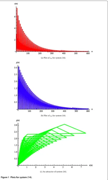
with initial conditionsx–= .,x–= .,x–= .,x–= .,x–= .,x–= .,x–= .,x–= .,x= .,y–= .,y–= .,y–= .,y–= .,y–= .,y–= .,y–=

.,y–= .,y= .. Moreover, in Figure , the plot ofxnis shown in Figure a, the plot

ofynis shown in Figure b, and an attractor of system () is shown in Figure c.

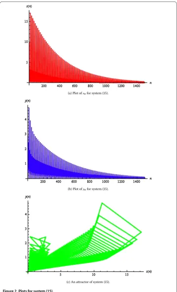
Example  Consider system () with initial conditionsx–= .,x–= ., x–= .,

x–= .,x–= .,x–= .,x–= .,x–= .,x–= .,x–= .,x–= .,x–= .,x–= .,x–= .,x–= .,x= .,y–= .,y–= .,y–= .,y–= .,

y–= .,y–= .,y–= .,y–= .,y–= .,y–= .,y–= .,y–= .,y–= .,

y–= .,y–= .,y= .. Moreover, choose the parametersα= ,β= ,γ= .,

α= ,β= ,γ= .. Then system () can be written as

xn+=

xn–  + ._i_=yn–i

, yn+=

yn–  + ._i_=xn–i

, n= , , . . . , ()

with initial conditionsx–= .,x–= .,x–= .,x–= .,x–= .,x–= .,

x–= .,x–= .,x–= .,x–= .,x–= .,x–= .,x–= .,x–= .,x–= .,

x= .,y–= .,y–= .,y–= .,y–= .,y–= .,y–= .,y–= .,y–= .,

y–= .,y–= .,y–= .,y–= .,y–= .,y–= .,y–= .,y= .. Moreover, in

Figure , the plot ofxnis shown in Figure a, the plot ofynis shown in Figure b, and an

attractor of system () is shown in Figure c.

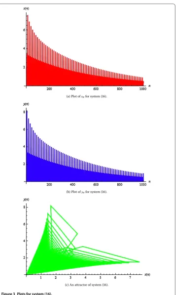
Example  Consider system () with initial conditionsx–= .,x–= .,x–= .,x–= .,x–= .,x–= .,x= .,y–= .,y–= .,y–= .,y–= .,y–= .,y–=

.,y= .. Moreover, choose the parametersa= ,b= ,c= ,a= ,b= ,

c= . Then system () can be written as

xn+=

yn–  + _i_=xn–i

, yn+=

xn–  + _i_=yn–i

, n= , , . . . , ()

with initial conditionsx–= .,x–= .,x–= .,x–= .,x–= .,x–= .,x= .,

y–= .,y–= .,y–= .,y–= .,y–= .,y–= .,y= .. Moreover, in Figure ,

the plot ofxnis shown in Figure a, the plot ofynis shown in Figure b, and an attractor

of system () is shown in Figure c.

Example  Consider system () with initial conditionsx–= .,x–= .,x–= .,

x–= .,x–= .,x–= .,x–= .,x–= .,x–= .,x–= .,x–= .,x–= .,x= .,y–= .,y–= .,y–= .,y–= .,y–= .,y–= .,y–= .,y–=

.,y–= .,y–= .,y–= .,y–= .,y= .. Moreover, choose the parameters

a= ,b= ,c= ,a= ,b= ,c= . Then system () can be written as

xn+=

yn–  + _i_=xn–i

, yn+=

xn–  + _i_=yn–i

, n= , , . . . , ()

with initial conditionsx–= .,x–= .,x–= .,x–= .,x–= .,x–= .,

x–= .,x–= .,x–= .,x–= .,x–= .,x–= .,x= .,y–= .,y–= .,y–= .,y–= .,y–= .,y–= .,y–= .,y–= .,y–= .,y–= .,y–=

.,y–= .,y= .. Moreover, in Figure , the plot ofxnis shown in Figure a, the

(18)

(a) Plot ofxnfor system ().

(b) Plot ofynfor system ().

(c) An attractor of system ().

(19)

(a) Plot ofxnfor system ().

(b) Plot ofynfor system ().

(c) An attractor of system ().

(20)

(a) Plot ofxnfor system ().

(b) Plot ofynfor system ().

(c) An attractor of system ().

(21)

(a) Plot ofxnfor system ().

(b) Plot ofynfor system ().

(c) An attractor of system ().

(22)

Conclusion

This work is a natural extension of [, , ]. In the paper, we have investigated the

qual-itative behavior of (k+ )-dimensional discrete dynamical systems. Each system has only

one equilibrium point which is stable under some restriction to parameters. The lineariza-tion method is used to show that equilibrium point (, ) is locally asymptotically stable. The main objective of dynamical systems theory is to predict the global behavior of a sys-tem based on the knowledge of its present state. An approach to this problem consists of determining the possible global behaviors of the system and determining which initial conditions lead to these long-term behaviors. In case of higher-order dynamical systems, it is crucial to discuss global behavior of the system. Some powerful tools such as semi-conjugacy and weak contraction cannot be used to analyze global behavior of systems () and (). In the paper, we prove the global asymptotic stability of equilibrium point (, ) by using simple techniques. We have carried out a systematical local and global stability analysis of both systems. The most important ﬁnding here is that the unique equilibrium point (, ) can be a global asymptotic attractor for systems () and (). Moreover, we have determined the rate of convergence of a solution that converges to the equilibrium point (, ) of systems () and (). Some numerical examples are provided to support our theo-retical results. These examples are experimental veriﬁcations of theotheo-retical discussions.

Competing interests

The authors have no competing interests. Authors’ contributions

All authors contributed equally in drafting this manuscript and giving the main proofs. Acknowledgements

This work was supported by the Higher Education Commission of Pakistan. Received: 3 October 2013 Accepted: 7 November 2013 Published:03 Dec 2013

References

1. Cinar, C: On the positive solutions of the diﬀerence equation systemxn+1=_yn1;yn+1=_xnyn

–1yn–1. Appl. Math. Comput.

158, 303-305 (2004)

2. Stević, S: On some solvable systems of difference equations. Appl. Math. Comput.218, 5010-5018 (2012) 3. Kurbanli, AS: On the behavior of positive solutions of the system of rational difference equationsxn+1=_ynxnxn–1_{–1 –1},

yn+1=_xnynyn–1_{–1 –1},zn+1=_ynzn1 . J. Diﬀer. Equ.2011, 40 (2011)

4. Stevi´c, S: On a third-order system of diﬀerence equations. Appl. Math. Comput.218, 7649-7654 (2012)

5. Bajo, I, Liz, E: Global behaviour of a second-order nonlinear diﬀerence equation. J. Diﬀer. Equ. Appl.17(10), 1471-1486 (2011)

6. Kalabuˆsić, S, Kulenović, MRS, Pilav, E: Dynamics of a two-dimensional system of rational difference equations of Leslie-Gower type. Adv. Differ. Equ. (2011). doi:10.1186/1687-1847-2011-29

7. Kalabuˆsić, S, Kulenović, MRS, Pilav, E: Global dynamics of a competitive system of rational difference equations in the plane. Adv. Differ. Equ.2009, Article ID 132802 (2009)

8. Kurbanli, AS, Çinar, C, Yalçinkaya, I: On the behavior of positive solutions of the system of rational diﬀerence equationsxn+1=_ynxnxn–1_{–1 +1}.yn+1=_xnynyn_{–1 +1}–1 . Math. Comput. Model.53, 1261-1267 (2011)

9. Din, Q: Dynamics of a discrete Lotka-Volterra model. Adv. Diﬀer. Equ.1, 1-13 (2013)

10. Din, Q, Donchev, T: Global character of a host-parasite model. Chaos Solitons Fractals54, 1-7 (2013)

11. Din, Q, Qureshi, MN, Khan, AQ: Dynamics of a fourth-order system of rational diﬀerence equations. Adv. Diﬀer. Equ.1, 1-15 (2012)

12. Din, Q, Khan, AQ, Qureshi, MN: Qualitative behavior of a host-pathogen model. Adv. Diﬀer. Equ. (2013). doi:10.1186/1687-1847-2013-263

13. Din, Q: Global behavior of a rational diﬀerence equation. Acta Univ. Apulensis34, 35-49 (2013)

14. Din, Q, Ibrahim, TF: Global behavior of a neural networks system. Indian J. Comput. Appl. Math.1(1), 79-92 (2013) 15. Qureshi, MN, Khan, AQ, Din, Q: Global behavior of third order system of rational diﬀerence equations. Int. J. Eng. Res.

Technol.2(5), 2182-2191 (2013)

16. El-Metwally, H, Elsayed, EM: Form of solutions and periodicity for systems of diﬀerence equations. J. Comput. Anal. Appl.15(5), 852-857 (2013)

(23)

18. Elsayed, EM, El-Metwally, HA: On the solutions of some nonlinear systems of diﬀerence equations. Adv. Diﬀer. Equ. (2013). doi:10.1186/1687-1847-2013-161

19. Elsayed, EM: Solution and attractivity for a rational recursive sequence. Discrete Dyn. Nat. Soc.2011, Article ID 982309 (2011)

20. Zhang, Q, Yang, L, Liu, J: Dynamics of a system of rational third order diﬀerence equation. J. Diﬀer. Equ. (2012). doi:10.1186/1687-1847-2012-136

21. Shojaei, M, Saadati, R, Adibi, H: Stability and periodic character of a rational third order diﬀerence equation. Chaos Solitons Fractals39, 1203-1209 (2009)

22. Sedaghat, H: Nonlinear Diﬀerence Equations: Theory with Applications to Social Science Models. Kluwer Academic, Dordrecht (2003)

23. Kocic, VL, Ladas, G: Global Behavior of Nonlinear Diﬀerence Equations of Higher Order with Applications. Kluwer Academic, Dordrecht (1993)

24. Pituk, M: More on Poincare’s and Perron’s theorems for diﬀerence equations. J. Diﬀer. Equ. Appl.8, 201-216 (2002)

10.1186/1687-1847-2013-354