R E S E A R C H
Open Access
Robust all-source positioning of UAVs based
on belief propagation
Xi Chen
*, Wenyun Gao and Jiabo Wang
Abstract
For unmanned air vehicles (UAVs) to survive hostile operational environments, it is always preferable to utilize all wireless positioning sources available to fuse a robust position. While belief propagation is a well-established method for all source data fusion, it is not an easy job to handle all the mathematics therein. In this work, a comprehensive mathematical framework for belief propagation-based all-source positioning of UAVs is developed, taking wireless sources including Global Navigation Satellite Systems (GNSS) space vehicles, peer UAVs, ground control stations, and signal of opportunities. Based on the mathematical framework, a positioning algorithm named Belief propagation-based Opportunistic Positioning of UAVs (BOPU) is proposed, with an unscented particle filter for Bayesian
approximation. The robustness of the proposed BOPU is evaluated by a fictitious scenario that a group of formation flying UAVs encounter GNSS countermeasuresen route. Four different configurations of measurements availability are simulated. The results show that the performance of BOPU varies only slightly with different measurements availability.
Keywords: UAV; Cooperative positioning; Belief propagation; Unscented particle filter
1 Introduction
Unmanned air vehicles (UAVs) require an accurate esti-mate of their positions, velocities, and attitudes in order to control themselves, navigate, and reason about their environment. The way this is achieved varies greatly from systems to systems. While most current UAV navigation systems rely on a combination of the Global Navigation Satellite Systems (GNSS) and an inertial measurement unit (IMU), there is a trend towards the use of all naviga-tion sources available to meet the endless pursuit of nav-igation robustness in the face of new threats and mission challenges [1-3].
For UAVs, besides GNSS signals, ranging with ground control stations and peer UAVs is readily achievable. Recently, signals of opportunities (SoOPs) from existing RF background infrastructure, such as digital terrestrial wireless TV signal, have also aroused much interests in the research community [4-6]. Under such a context, an innovative positioning algorithm is needed to fuse a right position utilizing all these measurements.
Existing positioning algorithms in the literature are enor-mous. Early pseudorange-only positioning algorithms for
*Correspondence: [email protected]
Space Center, Tsinghua University, Haidian District, Beijing, 100084, China
GNSS were based on iterative least square and Kalman filtering [7,8]. Extended Kalman filtering is a natural extension to Kalman filtering for solving nonlinear prob-lems using one-order linearization [9]. A big step forward for Kalman-based filtering is the invention of unscented Kalman filtering [10-12]. In cooperative positioning [13-20], nodes have not only pseudoranges from naviga-tion satellites but also ranging informanaviga-tion with wireless peers. Existing algorithms such as iterative least square and Kalman filters can be extended to cooperative posi-tioning, which leads to cooperative least square and coop-erative Kalman filtering algorithm [21]. In recent years, convex optimizations, including semidefinite program-ming (SDP) [22-25], sum of squares (SOS) relaxation [26,27], and distributed gradient algorithm, also found their place in cooperative positioning. Another category of positioning algorithms are Bayesian approaches with belief propagation as an outstanding representative. Belief propagation-based cooperative positioning was studied for wireless sensor networks, mobile ad hoc networks, vehicle ad hoc networks, etc. [28-31]. By jointly using ranges with peer nodes and pseudoranges from satel-lites, cooperative positioning dramatically improves the availability and accuracy of positioning, especially in GNSS-challenged environments.
Despite that positioning has been treated in various set-tings, there lack a study for positioning of UAVs with all wireless sources available, which is of fatal importance for UAVs to survive hostile operational environments. In fact, the US Defense Advanced Research Projects Agency (DARPA) had already initiated its All Source Positioning and Navigation (ASPN) program as emerging threat sce-narios become more sophisticated and widespread. Under all-source positioning context, flexibility and robustness, which allow for run-time join and leave of measurements, are of the first concern. Accuracy, however, is of the sec-ond concern. In existing work, algorithms based on belief propagations have proved to be the best candidate to meet the above requirements. While belief propagation is a well-established algorithm, it is not an easy job to han-dle the mathematics therein when all wireless positioning sources are considered.
For the above motivations, all-source positioning of UAVs based on belief propagations is studied in this work. The positioning sources include (1) pseudoranges and carrier phases from GNSS satellites, (2) ranges and closed-loop Doppler from peer UAVs, (3) ranging infor-mation and closed-loop Doppler with ground control stations [32], and (4) time difference of arrival (TDoA) from the signal of opportunities of background wireless infrastructure. The contributions are as follows: (1) A uni-fied mathematical framework for position and velocity estimation is developed, taking all the above measure-ments and their statistical characteristics. (2) Based on the mathematical framework, a positioning algorithm, named Belief propagation-based Opportunistic Position-ing of UAVs (BOPU), is proposed. (3) The factor products, which are mathematically intractable, are solved by an unscented particle filtering. For the accuracy performance of belief propagation with particle filters over Kalman fil-ters and cooperative least square algorithms has already been proved by existing work such as [28,29], we focused on evaluating the robustness of BOPU. Simulations are conducted with a fictitious scenario that a group of forma-tion flying UAVs are under the support of ground control stations but encounter GNSS countermeasuresen route. Four different configurations of measurements are sim-ulated and compared. The results show that the perfor-mance of BOPU varies only slightly with measurements availability.
The rest of the paper is organized as follows: Section 2 formulates the problem, Section 3 gives the details of the proposed positioning algorithm, Section 4 presents simu-lation results and discussions, and Section 5 concludes the paper.
2 Problem formulation
Consider a group of formation flying UAVs that are car-rying out a mission. All UAVs, together with their ground
control stations, form a wireless network. The set of UAVs is defined by a wireless node set M of cardinality |M|. Without loss of generosity, it is assumed that only one GNSS constellation is available with a set of satellitesSof cardinality|S|. There is also a set of SoOP signal sources G of cardinality|G|. The epoch sequence is denoted by t(0),t(1),. . .,t(k). For a selected wireless node m ∈ M,
denote by M(mk) the nodes that node mranges with, by S(mk) the subset of satellites m is in view, and by G(mg,k) the nodes thatmshares TDoA about SoOP signal source g ∈ G. The location of nodemat epochkis denoted by m(k) =[(mxk),my(k),(mzk)]T. The velocity of nodemat epoch kis denoted byv(mk) =[v(mxk),v(myk),v(mzk)]T. The clock bias of nodemwith reference to the selected GNSS constellation is denoted asb(mk)in meters, which notionally equals the product of the speed of light multiplying the clock bias of nodemin seconds. Define the state of nodemas the vec-tor x(mk) [((mk))T,(v
(k)
m )T,b(mk)]T. Node mperforms the following measurements:
1. Pseudorangeρs(→k)mfrom satellites∈S, which is in
the form
ρs(→k)m= s(k)−(mk) +bm(k)+bs(k)+ερ(ks) (1)
whereb(sk)represents the sum of correlated errors
which generally include tropospheric error, ionospheric error, and ephemeris error, whileερ(ks)
represents all uncorrelated errors following a Gaussian distribution.
2. Carrier phase elapsedφs(→k)mduring epochk and
k−1from satellites∈S, which is in the form
φs(→k)m= |φ|m+ε(φks) (2)
where|φ|mis the true value andεφ(ks)is the carrier phase observation Gaussian error.
3. Rangesr(nk↔)mwith neighborsn∈M(mk), which is in
the form
rn(k↔)m= (nk)−(mk) +ε(rk) (3)
wheren is the index of the neighbor andεr(k)is the
ranging error following a Gaussian distribution. A neighbor can be a peer UAV or a ground control station. The position of a UAV is unknown, but that of a ground control station is assumed to be known. Noter(nk↔)m=rm(k↔) n.
4. Closed-loop Doppler measurementfn(k↔)mwith
neighborsn∈M(mk). By closed-loop Doppler measurement [32], the clock differential of wireless neighbors is eliminated and the resultingfn(↔k)m
relative movement of the neighbor nodes involved,
whereλis the wavelength of the carrier used in
Doppler measurement, and
referring tog, which is in the form
dn(k→)m= meters, following a Gaussian distribution. Attaining TDoA measurement requires synchronization of
nodesn and m. Nowadays, one way to achieve this is
to use high-quality atomic clock re-synchronized at every departure. In such case,ε(dk)increases slowly as clock drift accumulates with time.
For brevity, we further define the following notations:
˜
The goal of the positioning is to find thea posteriori dis-tribution of x(mk) at each epochk, given all the available k, the final estimationμ(mk)is the statistical expectation of
x(mk)as
3 The proposed BOPU
3.1 The Bayesian inference
It is reasonable to assume that ranges with peer UAVs and the control stations are independent, and it is also often the case that the nodes inMmove independently. The pseudoranges are independent when ignoring b(sk).
The error induced by ignoringb(sk)will be discussed later. While the movement of a node can be measured read-ily by IMUs in many cases, it is not the case in all-source positioning because IMUs and wireless measurement are loosely coupled for flexibility. In this work, the movement of node m ∈ M is modeled as a second-order Markov process. With these assumptions, (7) can be rewritten as
px(mk)| ˜O(M1:k) To determine the marginal (7) recursively at each epochk, the integrand of (9) can be further decomposed as
p
Now for each nodem∈M, we define the following:
1. Υs,m(x(mk))p(ρs(→k)m|x(mk),φs(→1:km)), denoting the
pseudorange measurement model of nodem at
epochk.
2. Θs,m(x(mk))p(φ(s→k)m|x(mk)), representing carrier
phase measurement model of nodem at epoch k.
3. Γn,m(x(nk),x(mk))p(rn(k↔)m|x(mk),xn(k),fn(↔1:km)), denoting
the range measurement model of nodem with node
n at epoch k.
4. Ωng,m(xn(k),x(mk))p(d(ng→,k)m|xm(k),x(nk)), denoting the
TDoA measurement model of nodem to n with
reference to SoOP sourceg at epoch k.
5. Ψn,m(x(nk),x(mk))p(fn(↔k)m|x(mk),xn(k),fn(↔1:km)), denoting
the peer-to-peer Doppler measurements of nodesm
andn at epoch k.
6. Δm(x(mk),xm(k−2:k−1))p(x(mk)|xm(k−2:k−1)), denoting
dead reckoning of nodem from epochk−2 :k−1
tok.
With the above definitions, we have
pX˜(kM−1:k)| ˜O (1:k) M
∝
m∈M
⎛ ⎜
⎝
s∈S(mk)
Υm
x(k)m
×
n∈M(mk),n>m Γn,m
x(k)n ,x(k)m×
g∈G
n∈G(mg,k),n>m Ωng,m
x(k)n ,x(k)m
×
s∈S(mk)
Θs,m
x(k)m
n∈M(mk),n>m
Ψn,m
x(k)n ,x(k)m
×
n∈M(mk)
Δm
x(k)m ,x(km−2:k−1)px(km−2:k−1)| ˜O(kM−1)
⎞ ⎟ ⎠
(17)
With Equation 17, we have the factor subgraph of node mas given in Figure 1. The factor subgraphs of all nodes m∈M, when interconnected, make up the complete fac-tor graph. Figure 2 illustrates the complete facfac-tor graph of nodes of the simulation scenario given by Figure 3.
3.2 The sum product update rule
A belief propagation algorithm defines the sum product messages and their update rules over the factor graph. In our case, there are six classes of messages:
1. Dead-reckon messagehΔm→xm, associated to the
state of nodem from epochk−2 :k−1tok
2. Satellite pseudorange factor messageshΥs,m→xm,
associated to the pseudorange measurements, useful only in estimatingl(mk)andb(mk)
3. Satellite carrier phase factor messageshΘs,m→xm,
associated to the pseudorange measurements, useful only in estimatingl(mk)andv(mk)
4. Messages from range neighborshΓn,m→xm,
representing the positioning information from neighbors with range and closed-loop Doppler measurements
5. Messages from SoOP neighborshΩg
n,m→xm,
representing the positioning information from neighbors with TDoA measurement with reference
to the SoOP sourceg
6. Messages to peershxm→xn, wheren∈M
(k)
m which
nodem sends to all neighbors including range
neighbors and SoOP neighbors
The proposed positioning algorithm, named BOPU, includes two steps. The first step is to obtainp(x(m0)) at epoch 0, which is done by a cooperative least square positioning. The second step is to obtainp(x(mk)| ˜O
(1:k) M )at epoch k ≥ 1. Using all the above message definitions, the sum product update rule of the proposed positioning algorithm can be given as in Algorithm 1.
Algorithm 1 Belief propagation-based Opportunistic Positioning of UAVs
Require: Initial beliefsp(x(m0))at epoch 0,∀m∈M. Ensure: Updated beliefsp(x(mk)| ˜O
(1:k)
M ),∀m∈M 1: forepochk=1 toKdo
2: Acquire all observablesO˜(M1:k)available 3: Compute:
4: hΔm→xmusing Equations 19 and 20,∀m∈M 5: hxm→xnusing Equation 26,∀m∈M
6: Broadcasthxm→xnto all neighbors∀m∈M 7: foriterationi=1 toIdo
8: fornodesm∈Min parallel do
9: Receivehxn→Δn,mfrom all neighbors. 10: Compute:
11: hΓs,m→xmusing Equations 21 and 22; 12: hΘs,m→xm using Equation 24;
13: hxm→xn,∀n∈M
(k)
m using Equation 25. 14: Communicatehxm→xnton,∀n∈M
(k) m . 15: Compute:
16: hΓn,m→xmusing Equations 34 and 35; 17: hΩn,m→xm using Equation 40; 18: Update:
19: p(x(mk)| ˜O (1:k)
M )using Equation 41 20: end for
(k2:k1)
Figure 1The factor subgraph of nodem.The factor subgraphs of all nodesm∈Mmake up the complete factor graph.
3.3 The messages in parametric form
A compact parametric form of the messages involved in the proposed algorithm is needed to make it permis-sible to transmit over a wireless network with limited bandwidth, which are given below:
1. Dead-reckon messagehΔm→xmis associated to the
state of nodem from epochk−2 :k−1tok. From
Figure 1, we have
hΔm→xm ∝
S0-5: GNSS satellites
N0-5:Wireless nodes
N0'-1':Ground control stations
N1'
Figure 3The simulation scenario.A group of six UAVs are flying from a start point under the control of ground control stationN0to a destination with ground control stationN1, but experience a GPS countermeasure in the midway.
From its definition, the dead-reckon message is a Gaussian probability density function with mean
μ
Following (19), it is trivial to derive
Σ
xm(k)=4Σxm(k−1)+Σx(mk−2) (20)
2. Satellite factor messageshΥs,m→xmare associated to
the pseudoranges of nodem. The pseudorange of
nodem from satellite s is assumed to be bias free
except the receiver clock bias; thus, we have
hΥs,m→xm∝exp
whereσs2→mis the pseudorange error power of
satellites at node m andρˆ(sk)is the carrier phase
smoothed pseudorange, which can be expressed in a recursive form as [33]
ˆ
associated to satellite carrier phase measurements. For
where1m→sis the unit vector directed from nodem
to satellites,δfs(k)is the clock drift rate of satellites.
sends to all neighbors, in the following form:
hxm→xn∝hΔm→xm
At the initialization stage of each epoch,hΩg n,m→xm
It is hard to find the exact expression of Equations 25 and 26, so we approximate the result of message multiplication as a Gaussian distribution:
hxm→Δm,n≈
wherez is the normalization factor. In practice, the
values ofμ
x(m→nk) andΣx(m→nk) are approximated by an
unscented particle filtering as Algorithm 2, which will be disposed of later.
5. Messages from range neighborshΓn,m→xmrepresent
the contribution of ranging information from wireless neighbors. For the position of ground control stations are known,hΓn,m→xmassociated to
the ranging information of nodem to a control
stationn can be expressed as
hΓn,m→lm ∝exp
the Doppler smoothed range, which can be expressed in a recursive form as
ˆ
Ground control stations’ Doppler messageshΨn,m→xm
are associated to the Doppler information of nodem
to ground control stations. Similar tohΘs,m→xm, we
Messages from other UAVs whose positions are not known can be expressed as
hΓn,m→xm ∝
To find out the parametric form of this distribution, we follow a divide-and-conquer approach. First, we can see that the mean of positionl(mk)in this
valid point on the surface of the ball is restricted by
(rk)=μ l(m→nk) +r
(k)
thus, we have
6. Messages from SoOP neighborshΩg
n,m→xmrepresent
the contribution of TDoA measurements referencing
SoOP sourceg, which can be expressed as
hΩg
The mean positionl(mk)in this distribution is a ball with centerlgand radius||lg−μn→m|| −dn(k→)m, and
its covariance isΣ
x(n→mk) +σ
With Gaussian approximation, we can also calculate
p(x(mk)| ˜O (1:k)
M )using Algorithm 2.
Algorithm 2Message calculation using unscented parti-cle filter
Require: Initial estimateμˆxandΣˆx; Distributions of all incoming messages; N particles{z(i0)}Ni=1∼p(x(0));∀i,
2: Update the particle with UKF: 3: - Calculate 2na+1 sigma points:
4: Z(ik−1)=[z˜i(k−1),z˜(ik−1)±
(na+η)Σ(ik−1)] 5: - Propagate the particle into future:
6: Z(ik|k−1)=hs(Z(ik−1)) 11: -Incorporate new observations:
12: Σ˜yk,y˜k =
each factor using Equations 21, 22, 28, 29, 24, 30, and 25
20: Evaluate the importance weights of the new
particle:w(ik)=Πjpj(z(ik))/q(z (k) i ) 21: end for
22: Normalize the importance weights of all particles so thatΣiw(ik)=1
3.4 Calculating the factor products
The products of factors, i.e., Equations 25, 26, and 41, are mathematically intractable. This is a problem that per-meates in many disciplines of sciences. The most widely known methods are importance sampling [31], bootstrap particle filter [34], and unscented particle filters [35,36]. While importance sampling is convenient and attractive, it suffers from the sample degeneracy problem. Boot-strap filter and unscented particle filter try to avoid this degeneracy by context-aware resampling, which elimi-nates the particles having low importance weights and proliferates particles having high importance weights. A bootstrap particle filter uses state update information for resampling, while an unscented particle filter further improves the bootstrap particle filter by estimating the first- and second-order moments of the new state incor-porating new observations using unscented transform before resampling.
We present the variation of unscented particle fil-ter for calculating the factor products of this work in Algorithm 2. In Algorithm 2, na, η, Wjc0, and Wjc1 are parameters related to unscented transform.na = 7 is the number of states, which is 7 in our case.η = 3α2−na,
W0c0=η/(na+η), andW0c1=η/(na+η)+(3−α2)for Gaussian distributions. Forj = 1 to 2na,Wjc0 = Wjc1 = 1/[ 2(na+η)].
4 Simulations and discussions
4.1 Setup
For belief propagation combined with varied linear and nonlinear filters is widely available in the literature, we focused on evaluating the robustness of BOPU with some discussions on the appropriateness of the approximations in BOPU. Simulations are conducted by MATLAB with a fictitious scenario as given in Figure 3. In Figure 3, a group of six UAVs indexed by 0 to 5 are flying in a formation from a start point under the control of ground stationN0 to a destination with ground stationN1and a SoOP sourceG0 in view, but experience a GPS countermeasureen route.
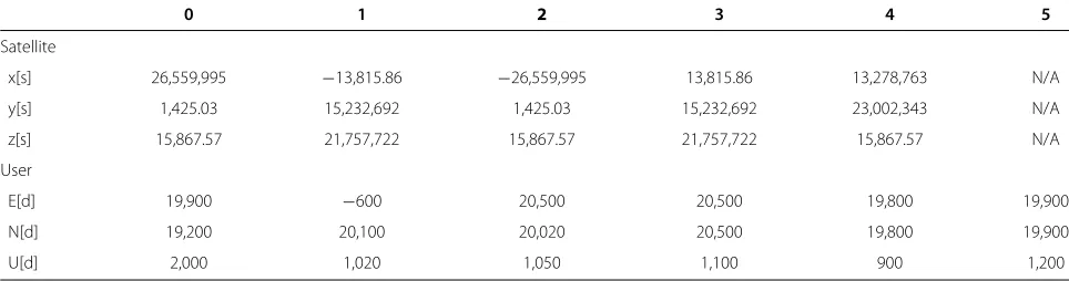
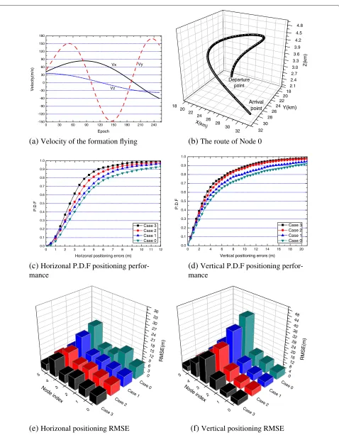
The positions of satellites in view are given in Table 1. All UAVs follow the same velocity but with a different point of departure as also given in Table 1. The velocity of the for-mation flying is given in Figure 4a, and the route of node 0 is given in Figure 4b. The simulated cases include the following:
• Case 0 : Whenever a node has at least four satellites in
view, it will not participate in the belief propagation but will offer the statistics of its own position. In addition, the measurements with the two ground
control stationsN0 andN1and the SoOP sourceG0
signal are not utilized. Case 0 reduces the positioning traffic over the wireless network to a minimum but is expected to have the poorest positioning
performance.
• Case 1 : All nodes take part in the belief propagation
process as stated in Algorithm 1 but do not utilize the measurements with the two ground control stations
N0andN1 and the SoOP sourceG0signal.
• Case 2 : All nodes take part in the belief propagation
process as stated in Algorithm 1, and the
measurements with the two ground control stations
N0andN1 and the SoOP sourceG0signal are used.
• Case 3 : All nodes take part in the belief propagation
process. Besides, the control stations also provide pseudorange differential corrections at each epoch and broadcast to other nodes. The differential corrections help effectively removeb(sk).
In the simulations, ground control stations 0 and 1 are placed at ENU(0, 0, 10)and ENU(50,000, 50,000, 10), respectively. The raw pseudorange observation error powerσs2→M = (3 m)2. The mean ofb(sk) is 6 m, and the error power ofb(sk) is(1 m)2. The error power of λ(δf) is(0.2 m/s)2, the error power ofλ(δφ)/(δt)is(0.1 m/s)2, the ranging error power with peers and ground con-trol stations is(3 m)2, and the TDoA measurement error power is set to (3 m)2, withα = 0.5. The SoOP source
Table 1 Satellites and UAV departure points in the simulation setup, where ENU(0,0,0) corresponds to LLH(116.3328,40.0018,100)
0 1 2 3 4 5
Satellite
x[s] 26,559,995 −13,815.86 −26,559,995 13,815.86 13,278,763 N/A
y[s] 1,425.03 15,232,692 1,425.03 15,232,692 23,002,343 N/A
z[s] 15,867.57 21,757,722 15,867.57 21,757,722 15,867.57 N/A
User
E[d] 19,900 −600 20,500 20,500 19,800 19,900
N[d] 19,200 20,100 20,020 20,500 19,800 19,900
U[d] 2,000 1,020 1,050 1,100 900 1,200
0 30 60 90 120 150 180 210 240 -150
-120 -90 -60 -30 0 30 60 90 120 150 180
Vz
Vy
Velocity(m/s)
Epoch Vx
(a)
Velocity of the formation flying
18 20 22 24 26 28 30 32 18
20 22
24 26
28 30
32
2.1 2.4 2.7 3.0 3.3 3.6 3.9 4.2 4.5 4.8
Y(km) Arrival
point Departure
point
Z(km)
X(k m)
(b)
The route of Node 0
0 1 2 3 4 5 6 7 8 9 10 11 12 0.0
0.1 0.2 0.3 0.4 0.5 0.6 0.7 0.8 0.9 1.0
P.D.F
Horizonal positioning errors (m)
Case 3 Case 2 Case 1 Case 0
(c)
Horizonal P.D.F positioning
perfor-mance
0 2 4 6 8 10 12 14 16 18 20 0.0
0.1 0.2 0.3 0.4 0.5 0.6 0.7 0.8 0.9 1.0
P.D.F
Vertical positioning errors (m)
Case 3 Case 2 Case 1 Case 0
(d)
Vertical P.D.F positioning
perfor-mance
0 1 2 3 4
5 0
3 6 9 12 15 18 21 24 27 30 33 36
Case
3
Case
2
Case
1
Case
0 RMS
E(m)
Nod e
index
(e)
Horizonal positioning RMSE
0 1 2 3 4
5 0
4 812
16 2024 28 32 36 40 44 48
Case
3
Case
2
Case
1
Case
0 RM
S E(m)
Nod e
index
(f)
Vertical positioning RMSE
G0 is placed at midway ENU(25,000, 25,000, 10). Nodes exchange time of arrival with wireless neighbors; thus, TDoA is also available between neighbors andD(G0,k)
m =
R(mk)\{N0,N1}.Te=1s.
4.2 Results and discussions
Figure 4 gives the simulation results. As can be seen, from case 0 to case 3, the positioning performance improves almost steadily. In case 0, node 0 and node 1 have at least four satellites, and they determine their position using a traditional weighted least square positioning algorithm in order to save communication bandwidth. Without itera-tions with node 0 and node 1, the positioning performance of other nodes is being restrained. In case 1, all nodes take part in the belief propagation process, which is help-ful in improving the positioning performance of all nodes (especially nodes 2 to 5), so the overall performance of case 1 is better than that of case 0. The outperformance of case 2 over case 1 comes from the full usage of all available observations, especially ranges and closed-loop Doppler with ground control stations, and TDoA observa-tions from SoOP sourceG0. The measurements with the ground control stationsN0,N1and SoOP sourceG0help improve geometric dilution of positioning in a big way. In case 3, ground control stations also generate corrections for pseudoranges, which directly improves the quality of pseudoranges, thus the positioning precision.
The positioning performance of all nodes is given in Figure 4e,f in terms of root mean square error (RMSE). It follows the fact that the more observables, the better pre-cision. In case 0, node 1 uses only the observation from four satellites in view, so its horizonal RMSE is even less than those of node 2 and node 3. Nodes 2 to 5, which have less than four satellites in view under some given GNSS interference, can still achieve positioning by utilizing the peer to peer measurements and the measurements with control stations. Node 5 experienced the strongest inter-ference. Without any satellite in view but with a better geometric position, node 5 achieved even better position-ing performance than nodes 3 and 4 that have satellites in view.
The results show that the performance of BOPU varies only slightly with different measurements availability. The main approximations made in the proposed BOPU are as follows: (1) The correlated errors of pseudorangesb(sk)are ignored in factorization. The simulation results of case 3 and case 2 show that such an approximation is accept-able. (2) The dead-reckon message (19) and (20) actually ignored nonzero off-diagonal values, and Equation 11 ignores the smoothing ofO˜(Mk−1)onx(mk−2). Such approxi-mations hold where the quality of observations dominates the positioning performance such as the cases in simula-tions. For UAVs, the positioning result using all wireless
sources is further coupled with IMU measurements to reach out for a better final result.
4.3 Algorithmic complexity
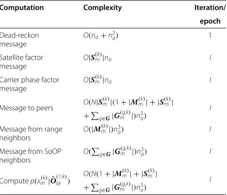
Given a nodemat epochk, we have one dead-reckon mes-sage, |S(mk)|satellite pseudorange factor messages, |M(mk)| messages from range neighbors, andg∈G|G(mg,k)| mes-sages from SoOP neighbors. It usesNparticles in UPF and I iterations in the product estimate. The core of UPF is UKF whose complexity isO(n3a)[37], wherenais the num-ber of states as stated before. The complexities of main computations in BOPU are listed in Table 2. As was shown in Table 2, the complexity of BOPU is dominated by mes-sage multiplications needed by mesmes-sages to peers, which scales asO(IN|S(mk)|(1+|M(mk)|+|Sm(k)|+g∈G|Gm(g,k)|)n3a).
5 Conclusions
Nowadays, UAVs are playing an increasingly important role both in the military and in civil affairs. Worries on the robustness of GNSS have also been increasing with the maturity of GNSS countermeasures and proliferation of wireless devices. With the aim of providing a better navigator for UAVs, we investigated the positioning of UAVs with all wireless sources via belief propagation with unscented particle filtering. By jointly using the measure-ments from GNSS satellites, peer UAVs, ground control stations, and signal of opportunities, the proposed algo-rithm, which is named BOPU, provides an improved positioning robustness and algorithmically proven high precision. By being opportunistic, BOPU allows for not only flexible variations of measurements availability but also agile compromise between wireless bandwidth con-sumption and positioning performance when put into practice.
Table 2 Computational complexity of nodemin the proposed BOPU
Computation Complexity Iteration/
epoch
Dead-reckon message
O(na+n2a) 1
Satellite factor message
O|S(mk)|na I
Carrier phase factor message
O|S(mk)|na I
Message to peers O(N|S
(k)
m|(1+ |Mm(k)| + |S(mk)|
I
+g∈G|G
(g,k)
m |)n3a)
Message from range neighbors
O(|M(mk)|)n3a) I
Message from SoOP neighbors
O(g∈G|G(mg,k)|)n3
a) I
Computep(x(mk)| ˜O
(1:k)
M )
O(N(1+ |M(mk)| + |S(mk)|
I
+g∈G|G
(g,k)
Competing interests
The authors declare that they have no competing interests.
Received: 27 May 2013 Accepted: 17 September 2013 Published: 25 September 2013
References
1. J Blanch, T Walter, P Enge, Satellite navigation for aviation in 2025. Proc. IEEE.100, 1821–1830 (2012)
2. R Garello, L Lo Presti, P di Torino, J Samson, Peer-to-peer cooperative positioning part I: GNSS-aided acquisition. Inside GNSS 55–63 (March/April 2012)
3. S Pullen, X Gao, GNSS jamming in the name of privacy-potential threat to GPS aviation. Inside GNSS 34–41 (March/April 2012)
4. A Dammann, S Sand, R Raulefs, inProceedings of the 20th European Signal Processing Conference (EUSIPCO). Signals of opportunity in mobile radio positioning (Bucharest, 27–31 Aug 2012), pp. 549–553
5. LP Gill, D Grenier, JY Chouinard, Use of XM radio satellite signal as a source of opportunity for passive coherent location. IET Radar, Sonar Navigation.5(5), 536–544 (2011)
6. M Robinson, R Ghrist, Topological localization via signals of opportunity. IEEE Trans. Signal Process.60(5), 2362–2373 (2012)
7. J Bao-Yen Tsui,Fundamentals of Global Positioning System Receivers: A Software Approach(Wiley, New York, 2004)
8. SJ Julier, JK Uhlmann, HF Durrant-Whyten, inProceedings of the American Control Conference,A new approach for filtering nonlinear systems. Seattle, 21–23 June 1995, pp. 1628–1632
9. T Perala, R Piche, inProceedings of the 4th Workshop on Positioning, Navigation and Communication (WPNC). Robust extended Kalman filtering in hybrid positioning applications (Hannover, 22–22 March 2007), pp. 55–63
10. EA Wan, R Van Der Merwe, inProceedings of the IEEE Adaptive Systems for Signal Processing, Communications, and Control Symposium (AS-SPCC). The unscented Kalman filter for nonlinear estimation (Alberta, 1–4 October 2000), pp. 153–158
11. X Zhai, F Qi, H Zhang, inProceedings of the Symposium on Photonics and Optoelectronics (SOPO). Application of unscented Kalman filter in GPS/INS (Shanghai, 21–23 May 2012), pp. 1–3
12. S Sarkka, On unscented Kalman filtering for state estimation of continuous-time nonlinear systems. IEEE Trans. Automatic Control.52(9), 1631–1641 (2007)
13. H Wymeersch, J Lien, MZ Win, Cooperative localization in wireless networks. Proc. IEEE.972, 427–450 (2009)
14. N Alam, A Tabatabaei Balaei, AG Dempster, A DSRC Doppler-based cooperative positioning enhancement for vehicular networks with GPS availability. IEEE Trans. Vehicular Technol.60(9), 4462–4470 (2011) 15. MA Caceres, F Sottile, R Garello, MA Spirito, inProceedings of the Personal,
Indoor and Mobile Radio Communications (PIMRC). Hybrid GNSS-ToA localization and tracking via cooperative unscented Kalman filter (Istanbul, 26–30 Sept 2010), pp. 272–276
16. J Yao, AT Balaei, M Hassan, N Alam, AG Dempster, Improving cooperative positioning for vehicular networks. IEEE Trans. Vehicular Technol.60(6), 2810–2823 (2011)
17. M Gholami, S Gezici, E Strom, Improved position estimation using Hybrid TW-TOA and TDOA in cooperative networks. IEEE Trans. Signal Process. 60(7), 3770–3785 (2012)
18. Y Qu, Q Tian, inProceedings of the International Conference on
Computational Aspects of Social Networks (CASoN). Multi-UAV cooperative positioning based on Delaunay triangulation (Taiyuan, 26–28 Sept 2010), pp. 401–404
19. Y Qu, Y Zhang, inProceedings of the IEEE/ASME International Conference on Mechatronics and Embedded Systems and Applications (MESA).
Fault-tolerant localization for multi-UAV cooperative flight (Qingdao, 15–17 July 2010), pp. 131–136
20. Y Qu, Y Zhang, Cooperative localization against GPS signal loss in multiple UAVs flight. J. Syst. Eng. Electron.22(1), 103–112 (2011)
21. Z Xiong, F Sottile, MA Caceres, R Garello, inProceedings of the IEEE-APS Topical Conference on Antennas and Propagation in Wireless Communications (APWC). Hybrid WSN-RFID cooperative positioning based on extended Kalman filter (Torino, 12–16 Sept 2011), pp. 990–993
22. N Wang, LQ Yang, inProceedings of the 24th International Technical Meeting of the Satellite Division of the Institute of Navigation (ION GNSS). Semidefinite programming for GPS (Oregon, 21–23 Sept 2011), pp. 2120–2126 23. A So, YY Ye, Theory of semidefinite programming for sensor network
localization. Math. Program.109, 367–384 (2007)
24. S Severi, G Abreu, G Destino, D Dardari, inProceedings of the IEEE Global Telecommunications Conference (GLOBECOM),Understanding and solving flip-ambiguity in network localization via semidefinite programming. Honolulu, 30 Nov–4 Dec 2009, pp. 1–6
25. WY Chiu, BS Chen, CY Yang, Robust relative location estimation in wireless sensor networks with inexact position problems. IEEE Trans. Mobile Comput.11, 935–946 (2012)
26. AY Alfakih, MF Anjos, V Piccialli, H Wolkowicz, Euclidean distance matrices, semidefinite programming and sensor network localization. Portugaliae Mathematica, 53–102 (2011)
27. H Waki, S Kim, M Kojima, M Muramatsu, Sums of squares and semidefinite program relaxations for polynomial optimization problems with structured sparsity. Siam J. Optimization.17(1), 218–242 (2006) 28. MA Caceres, F Penna, H Wymeersch, R Garello, Hybrid cooperative
positioning based on distributed belief propagation. IEEE J. Selected Areas Commun.29(10), 1948–1958 (2011)
29. F Sottile, H Wymeersch, MA Caceres, MA Spirito, inProceedings of the IEEE Global Telecommunications Conference (GLOBECOM). Hybrid
GNSS-terrestrial cooperative positioning based on particle filter (Houston, 5–9 Dec 2011), pp. 5–9
30. FR Kschischang, BJ Frey, HA Loeliger, Factor graphs the sum-product algorithm. IEEE Trans. Inf. Theory.47(2), 498–519 (2001)
31. D Barber,Bayesian Reasoning and Machine Learning(Cambridge University Press, Cambridge, 2012)
32. WM Smith, DC Cox, inProceedings of the IEEE Antennas and Propagation Society International Symposium (APSURSI). A closed-loop Doppler measurement for velocity estimation in mobile, multipath environments (Monterey, 20–25 June 2004), pp. 2203–2206
33. RR Hatch, inProceedings of the 3rd International Symposium on Satellite Doppler Positioning. The synergism of GPS code and carrier measurements (New Mexico, 8–12 Feb 1982), pp. 1213–1231 34. NJ Gordon, DJ Salmond, AFM Smith, Novel approach to
nonlinear/non-Gaussian Bayesian state estimation. IEEE Proc. Radar Signal Process.140(2), 107–113 (1993)
35. W Guo, C Han, M Lei. Improved unscented particle filter for nonlinear Bayesian estimation (Quebec, 9–12 July 2007), pp. 1–12
36. HW Li, J Wang, HT Su, Improved particle filter based on differential evolution. Electron. Lett.47(19), 1078–1079 (2011)
37. S Haykin,Kalman Filtering And Neural Networks(Wiley, New York, 2011), pp. 243–279
doi:10.1186/1687-6180-2013-150
Cite this article as:Chenet al.:Robust all-source positioning of UAVs based on belief propagation.EURASIP Journal on Advances in Signal Processing 20132013:150.
Submit your manuscript to a
journal and benefi t from:
7Convenient online submission
7Rigorous peer review
7Immediate publication on acceptance
7Open access: articles freely available online
7High visibility within the fi eld
7Retaining the copyright to your article