361 Copy right © The Society of Geomagnetism and Earth, Planetary and Space Sciences (SGEPSS); The Seismological Society of Japan; The Volcanological Society of Japan; The Geodetic Society of Japan; The Japanese Society for Planetary Sciences.
1. Introduction
It is generally recognized that the detailed time variation of tropopause structure is very important for studies of dynamical atmospheric properties, such as non linear wave processes and vertical transport of minor constituents. Indeed, recent developments in atmospheric chemistry suggest that the lowermost stratosphere and upper troposphere are more important for global chemical processes than was formerly thought (Holton et al., 1995).
The tropopause height is operationally determined by a conventional technique, represented by a rawinsonde ob-servation once to four times a day. However, its time resolution is not good enough to estimate fluctuations caused by short-period disturbances, such as atmospheric waves. Therefore, we are interested in application of a remote-sensing technique for tropopause detection.
In middle latitudes, there is significant seasonal and day-to-day variation in the tropopause structure. The mean tropopause height over Shigaraki, Japan (34°51′ N, 136°06′ E) varies from about 11 km in winter to 15 km in summer (Tsuda et al., 1991). Especially in winter months, the tropopause height often changes by as much as 4 or 5 km within a few days, affected by a passage of planetary scale disturbances. Under these circumstances the tropopause is not always well defined, since a front and multiple stable layers often confuse the classical picture of a single distinct boundary between the troposphere and stratosphere (e.g., Gage and Green, 1979).
An MST (mesosphere-stratosphere-troposphere) radar detects radiowave scattering by the refractive index fluc-tuations in a non-precipiting atmosphere. The MST radar echoes can be considered to arise from variations of the refractive index in the spatial volume defined by the trans-mitted pulse width and the antenna beam. For the 1–100 km altitude region these variations are attributed to a number of factors. The predominant factors include variations due to turbulence in humidity, temperature (or atmospheric density), and electron density. The relative contribution of these factors are strongly height dependent (Balsley, 1981).
In addition to the turbulent Bragg scattering, enhanced VHF echoes are received from a horizontally stratified atmospheric layer when the radar beam is steered into the vertical direction. This mechanism requires a spatial co-herence of the refractive index structure transverse to the radar wave vector (Balsley, 1981).
It has been reported by Tsuda et al. (1986) that profiles of both isotropic turbulent scattering and specular reflection are closely related to the background atmospheric stability. Therefore, the sharp increase in Brunt Väisälä frequency squared, N2, near the tropopause is associated with the enhancement of clear air echo intensity. Earlier studies detected a correlation between the tropopause and the alti-tude of sharp increase in vertical echo power or aspect sensitivity (Gage and Green, 1979, 1982; Röttger, 1980; Hocking et al., 1991). However, a detailed comparison between the N2 profile and echo power profiles has not been fully investigated yet. In this study, we compare these profiles with a height resolution as good as 150 m, and aim to find a statistical result on a possible height discrepancy
MU radar observations of tropopause variations by using clear air echo characteristics
E. Hermawan, T. Tsuda, and T. Adachi
Radio Atmospheric Science Center, Kyoto University, Uji, Kyoto 611, Japan
(Received August 12, 1996; Revised December 24, 1997; Accepted December 26, 1997)
We present in this paper the characteristics of clear air echoes revealed by the MU radar experiments in Shigaraki, Japan (34°51′ N, 136°06′ E). In particular, we study a relation between atmospheric stability, represented by Brunt Väisälä frequency squared, N2, and both the vertical echo power and the aspect sensitivity. On August 24–25, 1991, echo power was collected by steering the zenith angle of the antenna beam of the MU radar from the zenith to 28° with a step of 2°. Aspect sensitive echoes were detected in the lower stratosphere and some regions in the troposphere. We found that a ratio of vertical echo power to oblique echo power at 10° can represent the magnitude of aspect sensitivity. We compared profiles of both the vertical echo power and the aspect sensitivity with N2, inferred from a radiosonde sounding at the radar site. Cross correlation analysis indicates that a rapid increase of both vertical echo power and the aspect sensitivity near the tropopause usually coincides with a step-wise enhancement ofN2.
of clear air echoes, such as isotropic turbulence scattering and specular reflection. In Section 3, we present a brief description of the MU (middle and upper atmosphere) radar, together with observation techniques for use of clear air echoes, focusing on the aspect sensitivity. We also present in this Section a method for comparison between N2 and vertical echo power and aspect sensitivity using a cross correlation function (CCF). Then, in Section 4 we apply this technique for larger data-sets, collected in February 1987, June 1991, 1993 and 1994, in order to obtain a statistical result. Finally, we describe the summary and conclusions of this study in Section 5.
2. Fundamental Characteristics of Clear Air Echo
In this section we briefly introduce fundamental charac-teristics of isotropic turbulence scattering and specular reflection, which account for the clear air echoes detected with the MU radar. Further, we discuss their relationship to theN2 which is an index of atmospheric stability.
2.1 Isotropic turbulence scattering
The radar equation for isotropic turbulence scattering can be described as follows (e.g., Gage and Balsley, 1980):
P P A r
wherePs,Pt and Ae are the received power, the transmitted power and the effective area of the antenna, respectively. While,r and Δr are the range and the vertical extent of the volume given by half of radar pulse length, respectively. The volume radar reflectivity, ηturb for turbulence Bragg scattering is given as follows (Ottersten, 1969; Green et al., 1979; Hocking and Röttger, 1983; Hocking, 1985):
ηturb =0 38λ−
( )
21 3 2
. / Cn
whereλ is the radar wavelength and Cn2 is the refractive index structure constant, which depends upon the outer scale of turbulence, Lo, and the mean gradient of refractive index,M (Tatarskii, 1971):
Cn2 =2 8. L4 3o/ M2.
( )
3Note that M for a dry neutral atmosphere, which is the region of interest in the present study, can be approximated as follows (Ottersten, 1969):
M∝ρN2
( )
4whereρ is the air density. Furthermore, Lo4/3 was derived as (Hocking, 1985):
L4 3o/ =0 25. ε2 3/ N−2
( )
5whereε is the turbulence energy dissipation rate. Substituting Eqs. (3) and (5) into Eq. (2), we find:
2.2 Specular reflection
Considering a case of a one-way transmission from an antenna to its mirror image located at a distance 2r, the radar equation for a specular reflection was derived as (e.g., Gage and Green, 1978, 1979; Röttger, 1979; Gage and Balsley, 1980; Larsen and Röttger, 1982, 1985):
P P A
where ηref is the power reflection coefficient which was studied by VanZandt et al. (1978), VanZandt and Vincent (1983) Gage et al. (1985), assuming that the reflection is contributed by the background value of M and refractive index fluctuations with a scale of half of the radar wavelength. They derived ηref as:
ηref =CM E2
( )
2k( )
8whereC is a calibration constant which is determined by the radar wavelength and the height resolution of the radar sample volume, while E(2k) is the spatial density of re-fractive index variations with a scale of half the radar wavelength in the direction of the radar wave vector (VanZandt and Vincent, 1983). Substituting Eq. (4) into Eq. (8), we find:
ηref ∝ρ2E
( )
2k N4.( )
9The above relation was investigated by Röttger (1980), and it was further experimentally tested by Larsen and Röttger (1985) and Tsuda et al. (1988). Experimentally, Tsudaet al. (1988) showed that the vertical structure of ηref was mainly determined by M2, so the variation of E(2k) with height seems to be rather small. From Eq. (8), ηref was empirically found to be proportional to M2.
Near the tropopause ηturb and ηref can be inferred from oblique and vertical echo power, respectively. Considering Eqs. (6) and (9), intensity of both vertical and oblique echoes is closely related to the N2 structure near the tropopause, although it is also affected by the behavior of turbulence. We will show, however, in later section that the increase of the vertical echo power and the ratio of vertical to oblique echo power are correlated well with N2 profile.
3. Observation of Vertical and Oblique Echoes
3.1 MU radar observation
control-Fig. 1. Antenna beam directions for the MU radar observation on August 24–25, 1991. Full circles denote the beam positions.
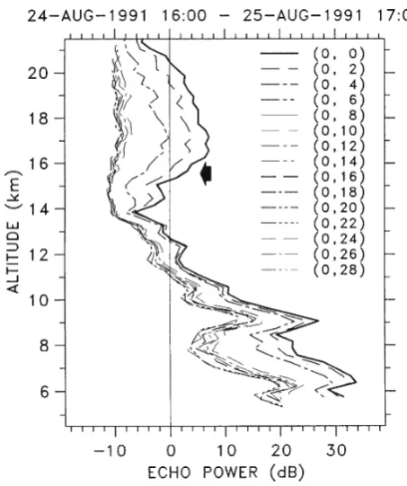
Fig. 2. Mean profiles of normalized echo power in 15 directions observed on August 24–25, 1991. Arrow at 15.5 km indicates the tropopause observed by a radiosonde at Shigaraki.
ler so that the MU radar is capable of executing a variety of observations.
For convenience we now define the normalized signal-to-noise ratio (SNR), Sθ, at a zenith angle, θ, after compen-sating for the range-squared effect and decrease of the effective antenna area as follows (Tsuda et al., 1997):
S P the range in km, respectively. Note that Sθ is normalized to the altitude of 10 km. Thus, the power reflection coefficient,
ηref, becomes proportional to Sθ.
We first present here a case study using data collected for about 25 hours on August 24–25, 1991 for detecting the zenith angle dependence of the echo power. We utilized a set of antenna beam directions; vertical and 14 beam positions at an azimuth angle of 0° (northward) changing the zenith angle from 2° to 28° every 2° as shown in Fig. 1. We also steered the 16-th beam toward east at the zenith angle of 10° to monitor the orthogonal wind component. Note that the antenna beam was steered sequentially into 16 positions in 16 IPP (inter pulse period), corresponding to about 6 msec, so the echoes were sampled essentially at the same time. 3.2 Zenith angle dependence of echo power
We describe here the zenith angle variations of echo power revealed by the MU radar observations. We expect that the reflection echo is the strongest in the vertical direction. While at a fairly large zenith angle, we may not receive the reflection any more, but isotropic turbulence scattering becomes dominant. Near the vertical direction both scattering and reflection contribute to the received signal. Therefore, we need to distinguish reflection echoes from isotropic scattering, by investigating zenith angle dependence of echo power.
This has been done by Röttger et al. (1981) using a
por-table VHF radar in conjunction with the Arecibo radar. More recently, Tsuda et al. (1986) used the MU radar to examine the aspect sensitivity of VHF backscattered power. During these experiments the MU radar scanned successively through a series of beam positions designed to define the angular dependence of backscattered power, Px (where x is the zenith angle) with 2 degree resolution.
Figure 2 shows mean profiles of normalized echo power,
Sθ observed on August 24–25, 1991. Note that the tropopause was identified at about 15.5 km by means of a radiosonde sounding. The vertical echo power was the largest in every height range, showing significant enhancement in com-parison with all other oblique echoes. An asymptotic profile of the vertical echo power generally decreased up to 14 km, increased at 14–17 km, reached the maximum at around 17 km, then decreased above. The oblique echoes at zenith angles larger than 6° showed similar profiles to the vertical echo in the troposphere but their profiles were overlapping with each other above 14 km.
sensi-Fig. 3. The log of N2 profile derived from Shigaraki radiosonde data launched at 21:58 LT on August 24, 1991 (left). Also shown the vertical echo power,Sv (center) and echo power ratio, Sv/S10 (right) derived from the MU radar observation in the same time. Solid line at 15.5 km indicates the tropopause height observed by a radiosonde at Shigaraki.
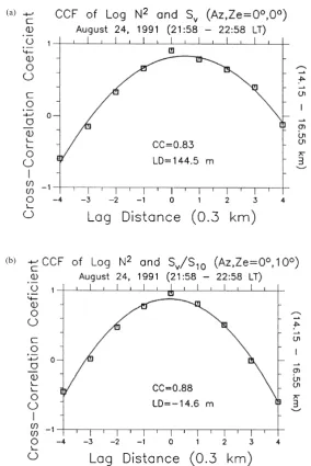
Fig. 4. Normalized cross correlation coefficient between log N2 and (a) S
v and (b) Sv/S10 for observation at 21:58–22:58 LT on August 24, 1991. (b)
tivity in later sections. It is noteworthy that the power ratio of the vertical echo to the isotropic scattering was small just above the tropopause and in the region above about 20 km (Hockinget al., 1990), and showed the maximum value of about 20 dB near 17 km (Tsuda et al., 1997).
3.3 Detailed comparison between echo power and N2
From a simultaneous radiosonde profile, we determined the tropopause height according to the conventional defini-tion of tropopause height from World Meteorological Orga-nization (WMO) that is, the tropopause is defined as the lowest level at which temperature lapse rate (dT/dZ) de-creases to 2 K/km or less and the dT/dZ averaged between this level and any level within the next 2 km does not exceed 2 K/km. We present in Fig. 3 profiles of N2,Sv and Sv/S
10
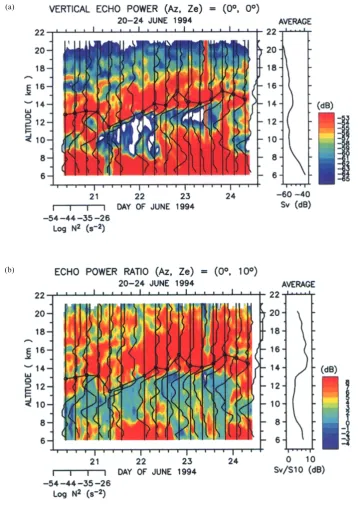
Fig. 5. Time-height section of (a) Sv and (b) Sv/S10 for observation on June 20–24, 1994. Also shown are the N2 profiles, and the tropopause height (–䊉–).
(b) (a)
determined on August 24, 1991, where a horizontal line at 15.5 km indicates the tropopause. Note that Sv and Sv/S10 are averaged during 21:58 and 22:58 LT. The tropopause (in-dicated by a horizontal line in Fig. 3) was associated with a pronounced discontinuity in atmospheric stability, which also coincided with the rapid increase in Sv and Sv/S10.
In order to investigate a correlation between N2 and Sv or
this technique to a larger data-set in the next section.
4. Statistical Comparisons between Echo Power andN2
With the MU radar we have been routinely measuring the troposphere and lower stratosphere for 4–5 days a month since 1984. The antenna beam is pointed into vertical and four orthogonal azimuths at 10° off the zenith. Among these data-sets, we selected here four periods in February 1987, June 1991, 1993 and 1994 when the temperature profile was simultaneously measured with a radiosonde at the radar site. We launched 7, 10, 8 and 16 radiosondes with an interval of 3–12 hours in the four observation periods, respectively, as summarized in Tables 1–4.
4.1 Time-height section of Sv and Sv/S10
We present in Figs. 5(a) and (b) a time-height section of
Sv and Sv/S10, respectively, in June 1994, together with a
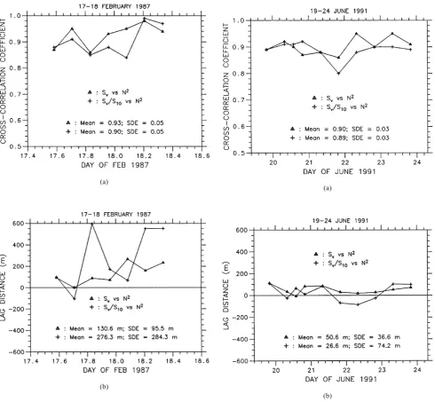
Fig. 7. The same as Fig. 6, but for on June 19–24, 1991. Fig. 6. Time variation of (a) CCF value and (b) lag distance for Sv vs.
N2 (䉱) and Sv/S10 vs. N2 (+) for observation on February 17–18, 1987.
(b) (a)
(b) (a)
about one hour for a radiosonde to reach the tropopause at about 14–15 km.
On June 21–23 large Sv values are generally detected in two height ranges, separated by a region with small Sv, which is a fairly common behavior of Sv (Tsuda et al., 1986). The correspondingN2 values in Fig. 5(a) sharply increased near the bottom of the upper region of the large Sv. While, from June 20 to beginning of June 21 and on June 24, Sv was not clearly depressed just below the tropopause, but showed rather irregular height variations. The N2 profiles in these periods did not also show a clear enhancement, but, sug-gested a multiple tropopause structure. From each radio-sonde sounding, the tropopause is determined according to the WMO definition, which was normally located just above the sharp increase of N2. Enhancement of both Sv and Sv/S
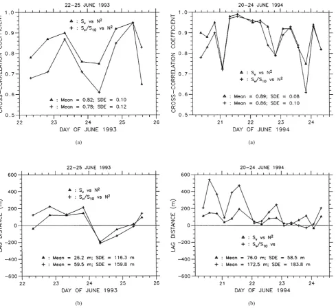
Fig. 9. The same as Fig. 8, but for on June 20–24, 1994. (b)
Fig. 8. The same as Fig. 7, but for on June 22–25, 1993. (b)
(a) (a)
4.2 CCF analysis between echo power and N2
We here present CCF analysis between N2 and Sv or Sv/S10, focusing on the height discrepancy in their enhancement. For an individual N2 profile, we compared the Sv and Sv/S
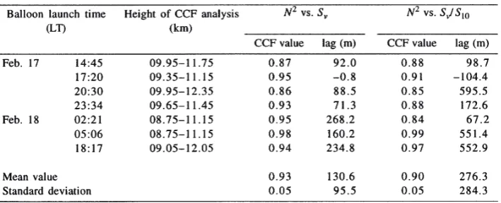
10 which are averaged for one hour starting from the balloon launch timing. Then, we selected a height range with a thickness of 2.1 to 4 km near the sharp increase in the N2 profile, then calculated CCF with N2 and Sv or Sv/S10. In Tables 1–4, we summarized the height range, maximum CCF value and lag distance for observations in February 1987, June 1991, 1993 and 1994, respectively.
For the results on February 17–18, 1978, the CCF value and lag distance are shown in Table 1 and Fig. 6. The mean CCF value during the period was as large as 0.93 and 0.90 forSv and Sv/S10, respectively, suggesting that these profiles resembled very well near the tropopause. However, the profiles were, on average, displaced vertically by 131 m and 276 m, respectively, that is, the increase in the echo power occurred slightly higher altitude than for N2. The lag
dis-tance was generally smaller for Sv than for Sv/S10, further, its standard deviation was smaller for Sv. On the other hand, the lag distance sometimes exceeded 500 m for Sv/S10.
Similar results are presented in Tables 2–4, and Figs. 7– 9 for data-sets collected in June 1991, 1993 and 1994. The results on June 19–24, 1991, shown in Table 2 and Fig. 7, indicate that the mean CCF value was 0.90 and 0.89 for Sv
andSv/S10, respectively, and the mean height discrepancy was as small as 51 m and 27 m, with the standard deviation of 37 m and 74 m, respectively. The agreement between the
N2 and echo power profiles were very good throughout the observation period.
For observations on June 22–25, 1993, considerable de-viations of CCF values were recognized as in Table 3 and Fig. 8, therefore, the mean value was only 0.82 and 0.78 for
N2 profiles, except for at 20:40 LT on June 22 and 8:13 LT on June 23, did not indicate a step-wise enhancement. In particular, for three cases between 20:25 LT on June 23 and 20:23 LT on June 24, the N2 value gradually increased, which made the CCF analysis less significant, resulting in small CCF values. Although the corresponding lag distance be-came negative, its significance seems to be uncertain.
For the comparison at 08:17 LT on June 24, 1993, the CCF value is as low as of 0.75 and 0.61 for Sv and Sv/S10,
re-spectively. Moreover, the increase in Sv and Sv/S10 occurred below the N2 enhancement by 150–300 m. Therefore, this particular case suggests that the N2 increase is not neces-sarily accompanied with enhancements of Sv and Sv/S10.
Table 4 and Fig. 9 show the results on June 19–23, 1994, when the largest number of radiosondes were launched. It is noteworthy that CCF values were very similar for Sv and Sv/
S10, including two cases at 02:22 LT on June 21 and at 20:32 LT on June 23, when the CCF value was less than 0.8. The
Table 2. The same as Table 1, but for on June 19–24, 1991.
Table 4. The same as Table 3, but for on June 20–24, 1994.
lag distance for Sv was persistently small during the obser-vation period, with the mean value of 76.0 m and its standard deviation of 59 m. However, for four cases on June 20–21, there was a considerable discrepancy in the lag distance betweenSv and Sv/S10. That is, the increase in Sv/S10 appeared higher than for Sv by 200–300 m, which simultaneously indicates that the Sv/S10 enhancement occurred higher than theN2 increase. These comparisons suggest that the sharp increase of Sv is not simultaneously associated with en-hancement of the aspect sensitivity.
The mean CCF values for total of 41 comparisons are shown in Tables 1–4 were 0.89 and 0.86 for Sv and Sv/S10, respectively. And, the corresponding lag distance was 71 m and 134 m, with standard deviation of 77 m and 176 m, respectively. These statistical results indicate that the en-hancement of Sv and Sv/S10 normally coincided with the enhancement of N2. Further, they occurred slightly higher altitude relative to the step-wise increase of N2, except for several cases when the N2 did not show a clear enhancement. We found that both Sv and Sv/S10 were correlated well with the increase of N2 near the tropopause, although the lag distance was relatively larger for the latter.
Röttger (1980) showed that the echo power increase occurred higher than the tropopause by 300–750 m from SOUSY-VHF-Radar observations. Gage and Green (1979) also found that the radar tropopause was higher than ra-diosonde results by 300 m. Our analysis, focusing on the detailed variations in this region near the tropopause, clari-fied that the height difference between N2 and Sv or Sv/S10 is as small as 71 m and 134 m, respectively.
5. Summary and Conclusions
This study is mainly concerned with the characteristics of clear air echo intensity near the tropopause, by means of the MU radar observations and simultaneous radiosonde sounding. Earlier theoretical studies on the scattering of VHF radiowaves caused by the refractive index fluctuations
of the atmosphere suggest that the echo intensity of both isotropic turbulence scattering and specular reflection is related to N2.
We first analyzed a campaign observation on August 24– 25, 1991, where vertical and oblique echo were obtained at 0°–28° by steering the antenna beam of the MU radar with a step of 2°. The echo power at zenith angles 0°, 2° and 4° in the lower stratosphere and some regions in the troposphere was significantly larger than that at other larger zenith angles. A ratio of vertical echo power, Sv, which was the largest in the entire height range, to oblique echo power at 10°,Sv/S10, can represent the aspect sensitivity.
We compared profiles of both Sv and Sv/S10 with N2, in-ferred from a radiosonde sounding at the radar site, and found that near the tropopause a large enhancement of both
Sv and Sv/S10 coincides with a step-wise increase in N2 profile. Cross correlation analysis between N2 and Sv or Sv/
S10 shows the maximum CCF values of 0.83 and 0.88, respectively. However, the CCF also suggests that the sharp increase of Sv and Sv/S10 occurred 145 m higher and 15 m lower than that for N2.
From the monthly MU radar observations in the tropo-sphere and lower stratotropo-sphere, routinely continued 4–5 days every month since 1984, we selected the data-sets in Febru-ary 1987 and June 1991, 1993 and 1994, when radiosondes were launched every 3–12 hours during the radar experiment. Time evolution of Sv clearly correlated with the variations of
N2 profiles. It is noteworthy that the meteorologically defined tropopause was not necessarily coincided with the step-wise increase in N2, but, it was determined slightly higher.
We analyzed CCF for total of 41 profiles, and obtained the mean CCF values of 0.89 and 0.86 for Sv and Sv/S10, re-spectively. The CCF analysis shows that the increase of Sv
that is, for 11 out of 41 comparisons its enhancement occurred below the N2 increase by 25–150 m.
The observed good relation between N2 and the echo power characteristics could be applied to a development of new observational technique for the atmospheric stability structure near the tropopause with good time and height resolution. For further development of this technique, we need to conduct a coordinated observation between the MST radar and a real-time monitoring of temperature structure with, for example, RASS (radio acoustic sounding system) technique.
Acknowledgments. We are grateful to Dr. T. Nakamura of RASC, Kyoto University for his useful suggestions and comments. The MU radar belongs to and is operated by Radio Atmospheric Science Center, Kyoto University.
References
Balsley, B. B., The MST technique—a brief review, J. Atmos. Terr. Phys., 43, 495–509, 1981.
Fukao, S., T. Sato, T. Tsuda, S. Kato, K. Wakasugi, and T. Makihira, The MU radar with an active phased array system: 1. Antenna and power amplifiers,Radio Sci.,20, 1155–1168, 1985a.
Fukao, S., T. Sato, T. Tsuda, S. Kato, K. Wakasugi, and T. Makihira, The MU radar with an active phased array system: 2. In-house equipment, Radio Sci.,20, 1169–1176, 1985b.
Gage, K. S. and B. B. Balsley, On the scattering and reflection mechanisms contributing to clear air radar echoes from the troposphere, stratosphere, and mesosphere, Radio Sci.,15, 407–416, 1980.
Gage, K. S. and J. L. Green, Evidence for specular reflection from monostatic VHF radar observations of the stratosphere, Radio Sci.,13, 991–1001, 1978.
Gage, K. S. and J. L. Green, Tropopause detection by partial specular reflection with VHF radar, Science.,203, 1238–1240, 1979. Gage, K. S. and J. L. Green, An objective method for the determination
of tropopause height from VHF radar observation, J. Appl. Meteorol., 21, 1150–1154, 1982.
Gage, K. S., W. L. Ecklund, and B. B. Balsley, A modified Fresnel scattering model for parameterization of Fresnel returns, Radio Sci.,20, 1493–1501, 1985.
Green, J. L., K. S. Gage, and T. E. VanZandt, Atmospheric measurements by VHF pulsed Doppler radar, IEEE Transactions on Geoscience Electronics,GE-17, 1979.
Hocking, W. K., Measurement of turbulent energy dissipation rates in the middle atmosphere by radar techniques: A review, Radio Sci.,20, 1403–
1422, 1985.
Hocking, W. K. and J. Röttger, Pulse length dependence of radar signal
larly above 15 km altitude, Radio Sci.,25, 613–627, 1990.
Hocking, W. K., S. Fukao, M. Yamamoto, T. Tsuda, and S. Kato, Viscosity waves and thermal-conduction waves as a cause of “specular”
reflectors in radar studies of the atmosphere, Radio Sci.,26, 1281–1303, 1991.
Holton, J. R., P. H. Haynes, M. E. McIntyre, A. R. Douglass, R. B. Rood, and L. Pfister, Stratosphere-Troposphere Exchange, Rev. Geophys.,33, 403–440, 1995.
Larsen and J. Röttger, VHF and UHF Doppler radars as tools for synoptic research,Bull. Amer. Meteor. Soc.,63, 996–1008, 1982.
Larsen and J. Röttger, Observations of frontal zone and tropopause structures with a VHF Doppler radar and radiosondes, Radio Sci.,20, 1223–1232, 1985.
Ottersten, H., Mean vertical gradient of potential refractive index in turbulent mixing and radar detection of CAT, Radio Sci.,4, 1247–1249, 1969.
Röttger, J., VHF radar observations of a frontal passage, J. Appl. Meteorol., 18, 85–91, 1979.
Röttger, J., Structure and dynamics of the stratosphere and mesosphere revealed by VHF radar investigations, Pure and Appl. Geophys.,118, 494–527, 1980.
Röttger, J., P. Czechowsky and G. Schmidt, First low-power VHF radar observations of tropospheric, stratospheric and mesospheric winds and turbulence at the Arecibo Observatory, J. Atmos. Terr. Phys.,43, 789–
800, 1981.
Tatarskii, The effects of the turbulent atmosphere on wave propagation, U.S. Dept. of Commerce, 1971.
Tsuda, T., T. Sato, K. Hirose, S. Fukao, and S. Kato, MU radar observa-tion of the aspect sensitivity of backscattered VHF echo power in the troposphere and lower stratosphere, Radio Sci.,21, 971–980, 1986. Tsuda, T., P. T. Pay, T. Sato, S. Kato, and S. Fukao, Simultaneous
observations of reflection echoes and refractive index gradient in the troposphere and lower stratosphere, Radio Sci.,23, 655–665, 1988. Tsuda, T., T. E. VanZandt, M. Mizumoto, S. Kato, and S. Fukao, Spectral
analysis of temperature and Brunt Väisälä frequency fluctuations observed by radiosondes, J. Geophys. Res.,96, 17265–17278, 1991. Tsuda, T., T. E. VanZandt, and H. Saito, Zenith-angle dependence of
VHF specular reflection echoes in the lower atmosphere, J. Atmos. Terr. Phys.,59, 761–775, 1997.
VanZandt, T. E. and R. A. Vincent, Is VHF Fresnel reflectivity due to low-frequency buoyancy waves?, Handbook for MAP, Middle Atmosphere Program, University of Illinois, Urbana,9, 78–80, 1983.
VanZandt, T. E., J. L. Green, K. S. Gage, and W. L. Clark, Vertical profiles of reflectivity turbulence structure constant: Comparison of observations by the Sunset radar with a new theoretical model, Radio Sci.,13, 819–829, 1978.